Multisensory Integration during Motor Planning

Abstract

When planning goal-directed reaches, subjects must estimate the position of the arm by integrating visual and proprioceptive signals from the sensory periphery. These integrated position estimates are required at two stages of motor planning: first to determine the desired movement vector, and second to transform the movement vector into a joint-based motor command. We quantified the contributions of each sensory modality to the position estimate formed at each planning stage. Subjects made reaches in a virtual reality environment in which vision and proprioception were dissociated by shifting the location of visual feedback. The relative weighting of vision and proprioception at each stage was then determined using computational models of feedforward motor control. We found that the position estimate used for movement vector planning relies mostly on visual input, whereas the estimate used to compute the joint-based motor command relies more on proprioceptive signals. This suggests that when estimating the position of the arm, the brain selects different combinations of sensory input based on the computation in which the resulting estimate will be used.

Introduction

Sensory channels often provide redundant information, as is the case when both visual and proprioceptive feedback encode the position of the arm. Recent studies suggest that when integrating redundant signals, the brain forms a statistically optimal (i.e., minimum-variance) estimate by weighting each modality according to its relative precision. Minimum-variance models have been shown to account for human performance when subjects integrate vision and touch (Ernst and Banks, 2002), vision and audition (Ghahramani, 1995), and other combinations of sensory input (Welch et al., 1979; Jacobs, 1999; van Beers et al., 1999). These models are appealing because they provide a simple rule by which the brain could minimize errors attributable to sensory noise.

Although these models predict a single, optimal estimate, other lines of research suggest that the brain forms multiple and sometimes inconsistent estimates of environmental variables. For example, studies of patients with temporal or parietal lobe lesions indicate that the brain has independent streams of visual processing for perceptual as opposed to motor tasks (Goodale and Milner, 1992; Milner and Goodale, 1995). Studies of reaching to illusory objects have shown a similar dissociation in normal subjects (Aglioti et al., 1995; Haffenden et al., 2001). These results suggest that sensory signals might be processed differently depending on how they will be used.

Here we focus on the integration of visual and proprioceptive feedback from the arm before the execution of a reach. This study seeks to quantify how vision and proprioception are combined to estimate arm position and to determine whether the nervous system uses a single criterion (e.g., minimum-variance) to combine the two modalities, or if different combinations of sensory input are selected at each stage of motor planning. Our approach is to displace the visual feedback from the arm before movement onset and use the resulting movement errors to infer the relative weighting given to each sensory modality.

Our analysis relies on the premise that estimates of arm position (a term that we use to denote both the position of the fingertip and the angles of the joints) are used in two separate stages of motor planning and on the observation that distinct patterns of movement errors would result from position misestimation at each stage. In the first stage, a desired movement vector in visual (extrinsic) space is computed by subtracting the estimated initial arm position from the target location. Clearly, if this initial position is misestimated, the planned movement vector will be wrong (Rossetti et al., 1995). We will refer to the resulting error pattern, illustrated in Figure 1, A and B, as movement vector (MV) error. A second and perhaps less intuitive source of error is the transformation of the extrinsic movement vector into a joint-based (intrinsic) motor command (Ghilardi et al., 1995; Goodbody and Wolpert, 1999). This transformation is equivalent to evaluating an inverse model of the arm (Jordan, 1996) and requires an estimate of the arm's initial position. Position misestimation at this stage of reach planning will also result in movement errors. An example is illustrated in Figure 1C. A leftward shift in estimated arm position causes the subject to choose the wrong motor commands (an extension or flexion of the elbow), resulting in clock- wise (CW) errors in initial reach direction (see Fig. 1D). We will refer to this type of error as inverse model (INV) error. Although both MV and INV error result from misestimation of the arm's initial position, the two stages of motor planning may rely on two different position estimates.

Figure 1.

Misestimation of arm position results in two types of reach errors. A, Errors resulting from a leftward shift in the position estimate used to plan the movement vector. The planned movement directions (gray arrows) differ from the actual hand-to-target directions (dashed lines). The pattern of directional errors (colored arrows) is plotted as a function of target direction in B. A rightward shift would produce the opposite pattern (see Fig. 4 B). CW, Clockwise; CCW, counterclockwise. C, Errors resulting from a leftward shift in the position estimate used to transform the desired movement vector into a joint-based motor command. The directions of the achieved movements (black arrows) differ from the planned movement directions (gray arrows). The pattern of errors (colored arrows) is plotted as a function of planned movement direction in D. The leftward shift shown here produces CW errors for all planned reach directions. A rightward shift would produce CCW errors.

The integration of vision and proprioception at these two planning stages has never been characterized independently and simultaneously. Here we show that shifts of visual feedback before movement onset result in a combination of the MV and INV error patterns. Fitting the observed errors with simple mathematical models of motor planning allows us to quantify the relative contributions of vision and proprioception to the position estimate used at each planning stage.

Materials and Methods

Experimental setup and data collection

Seven right-handed subjects (two female, five male) participated in the experiment. Subjects were 26-33 years of age and were healthy with normal or corrected-to-normal vision. All subjects were naive to the purpose of the experiment and were paid for their participation.

The task was performed with the right arm, which rested on a shoulder-height table (see Fig. 2 A). To minimize friction, the arm was supported by air sleds (0.73 kg upper arm, 1.18 kg forearm). The wrist was pronate and fixed in the neutral position with a brace, and the index finger was extended in a custom splint that permitted only vertical movement of the digit. Both shoulders were lightly restrained to minimize movement of the torso. This configuration restricted movement of the arm to 2 df and to a horizontal plane just above the table (Fig. 1). Arm position could therefore be expressed interchangeably as x, a two-dimensional vector representing the Cartesian position of the fingertip, or as θ, a two-dimensional vector composed of the shoulder and elbow angles.

Figure 2.

Data collection and experimental design. A, Side view of the behavioral apparatus. For clarity, the tactile start points (dowels) and drape are not shown. B, Top view of a subject showing the placement of the infrared markers (gray dots). Joint angles (θ₁ and θ₂) were computed from these five positions and from the measured lengths of the upper and lower arm (L₁ and L₂). C, Workspace configuration. The dowels marking the three tactile start points (gray dots) were arranged in a line parallel to the subject's left-right axis and were spaced 6 cm apart. L, Leftstart point; C, center start point; R, rightstart point. D, Trial types. Grid entries indicate the tactile start point (left column) and the presence of a leftward or rightward shift (right column) in each trial type.

Three dowels, which served as tactile start points, were fixed a few centimeters above the plane of movement and could only be reached when the subject raised his or her fingertip from the splint. The visual feedback spot and target circles were presented via a mirror and rear-projection screen such that the images appeared to lie in the plane of the arm. A liquid crystal display projector (1024 × 768 pixels) with a 75 Hz refresh rate was used. A drape prevented vision of the arm, the table, and the dowels. Five infrared-emitting diodes were attached to each subject's arm and torso (Fig. 2 B). Arm position data were sampled at 120 Hz using an infrared tracking system (OPTOTRAK, Northern Digital, Waterloo, Ontario). Elbow and shoulder angles were computed using the five marker positions and the lengths of the upper arm and forearm, which were measured using standard anatomical landmarks.

Task design

The workspace contained the three start points and eight targets (Fig. 2C). The dowels marking the start points were spaced 6 cm apart, and the center dowel was positioned ∼40 cm from the subject's chest and slightly to the right of midline. The targets were evenly arrayed on a circle of radius 18 cm centered at the middle start point.

The experiment consisted of 160 trials. At the beginning of every trial, text reading “Left,” “Center,” or “Right” appeared briefly at a random location on the screen, instructing the subject to locate the appropriate dowel with his or her raised index finger. The trial continued when (1) the fingertip was within 1 cm of a point directly below the appropriate dowel and (2) the fingertip was lowered back to the splint, where it remained for the rest of the trial. At this point, the visual feedback spot (a white circle of radius 3 mm) appeared at the location of the subject's fingertip or displaced to the left or right by 6 cm. Simultaneously, a red target of radius 5 mm appeared at one of the eight target locations. After a variable delay of 500-1500 msec, the target turned green, cueing the subject to begin the reach. Subjects were instructed to reach directly and accurately to the target. When the fingertip had moved 5 mm from its starting point, the feedback spot was extinguished, and the remainder of the reach was performed without visual feedback. The trial ended when the tangential fingertip velocity fell below 1.2 mm/sec. The target remained illuminated for the entire reach.

The experiment was composed of five trial types (Fig. 2 D). In Left-Zero, Right-Zero, and Center-Zero trials, reaches were made from each of the three start points with no visual shift. In Center-Left and Center-Right trials, reaches from the center start point were made with 6 cm leftward and rightward visual shifts, respectively. Note that with these shifts, the feedback spot appeared at the locations of the left and right tactile start points. The experiment consisted of four reaches to each of the eight targets under these five conditions in a pseudorandom order, totaling 4 × 8 × 5 = 160 reaches. To prevent subjects from adapting to the visual shifts, trials with left shifts, right shifts, and veridical feedback were pseudorandomly interleaved, and no two consecutive trials included the same shift. Adaptation was also unlikely because only twofifths of the trials included shifts and because the visual feedback (shifted or veridical) was available only at the start point.

A set of 32 familiarization trials preceded the actual experiment. First, a block of 24 Left-Zero, Center-Zero, and Right-Zero trials was performed with continuous visual feedback to acclimate subjects to the task and experimental apparatus. Next, a block of eight trials was performed with initial feedback only to familiarize subjects with reaching in the absence of visual feedback. After the experiment was completed, subjects were asked whether they felt that the location of the visual feedback spot ever deviated from the location of their fingertip. All but one subject reported being unaware of any visual shift. The remaining subject (HA) reported that the location of the feedback spot seemed to have been displaced on a small number of trials (fewer than five).

Data analysis and model fitting

Trajectory analysis. Arm position data were smoothed with a low-pass Butterworth filter with a cutoff frequency of 6 Hz, and the fingertip velocity and acceleration were successively computed using numerical differentiation (first differences). We quantified initial reach directions by determining the angle of the instantaneous velocity or acceleration vector at the point along the trajectory at which the tangential velocity first exceeded 40% of its peak value.

Modeling the initial movement direction. In building an explicit model of reach planning, we had to specify which extrinsic and intrinsic variables are used. Behavioral studies have variously suggested that reach planning uses either kinematic (Flash and Hogan, 1985; Atkeson and Hollerbach, 1985) or dynamic (Uno et al., 1989; Gordon et al., 1994b) variables, and neurophysiological findings have been cited to support both hypotheses (Cheney and Fetz, 1980; Georgopoulos et al., 1982; Todorov, 2000). We therefore fit our data twice, using the two models shown in Figure 3. In the velocity command model, the motor command is specified kinematically (as joint angle velocities), whereas in the torque command model the motor command is specified dynamically (as joint torques).

Figure 3.

Two models of feedforward motor planning. Arm position estimates X̂_INV are computed by combining visual and proprioceptive signals. A movement vector describing the desired direction of the initial velocity (Ẋ^*) or acceleration (ẍ^*) of the hand is computed by subtracting X̂_MV from the target location x^*. An inverse model transforms this desired extrinsic vector into an intrinsic motor command specifying joint angle velocities ( ) or torques (τ), depending on the model being implemented. This transformation makes use of a second position estimate, X̂ and X̂_INV. Finally, the motor command is executed, determining the initial hand trajectory. Note that the loop through the “Vision” and “Proprioception” boxes does not imply feedback control; in these models, the position estimates are only used to plan the plan the initial, feedforward component of a movement.

The goal of these models is to understand how visual and proprioceptive signals from the sensory periphery combine to guide the initial, feedforward component of the reach. In these models, only the initial velocities or accelerations of movements are computed, and feedback control is not modeled. We assume that the CNS weights the visual (x̂_vis) and proprioceptive (x̂_prop) position estimates and adds them to create two estimates of the position of the arm, x̂_MV (“movement vector”) and x̂_INV (“inverse model”):

1

2

The estimate x̂_MV is used to determine the desired movement vector in both models. This vector specifies desired initial fingertip velocity in the velocity command model and the desired initial fingertip acceleration in the torque command model. The second estimate, x̂_INV, is used to convert the desired movement into an intrinsic motor command. This command is expressed as joint velocities in the velocity command model and as joint torques in the torque command model. In both models, therefore, the weighting parameters α_MV and α_INV characterize sensory integration at the two stages of reach planning.

Velocity command model. In the velocity command model, the planned movement vector is defined as the desired initial velocity of the fingertip (ẋ^*). The direction of this velocity is specified by:

3

where x represents the angle of vector x, x*_d represents the location of target d ∈ [1,..., 8], x̂_MV is the estimated hand position defined in Equation 1, and ω_d is an angular offset from the straight line connecting the estimated initial position and target x*_d. We included the ω_d terms to account for the fact that natural, unperturbed reaching movements are slightly curved (Soechting and Lacquaniti, 1981; Atkeson and Hollerbach, 1985; Uno et al., 1989), resulting in initial reach directions that differ from the target direction. This baseline bias was fit from the Center-Zero trials: each ω_d was set to the average angular difference between the initial velocity direction and the target direction for target x*_d. Equation 3 does not specify the magnitude of ẋ^*, because ultimately only the predicted direction of movement will be compared with the data. Note that the pattern of errors in ẋ^* resulting from misestimation of x̂_MV is the MV error shown in Figure 1, A and B.

Given a desired Cartesian fingertip velocity ẋ^*, the ideal joint angle velocity command would be:

where the Jacobian matrix J(θ) is the gradient of the fingertip location with respect to the joint angles:

The kinematics equation x = K(θ) describes the mapping from joint angles to fingertip locations. Note that because the arm is restricted to planar, two-joint movements, both the kinematics and the Jacobian are invertible. Because the internal inverse model must rely on an estimate of the position of the arm (x̂_INV), the implemented motor command will be:

4

where:

Finally, this joint velocity command is executed, and the arm moves with an initial fingertip velocity determined by the Jacobian (evaluated at the true arm position):

5

This model predicts that the initial velocity ẋ will be distorted from the desired velocity ẋ^* if the arm position is misestimated. The matrix , which we will call the velocity distortion matrix, determines the INV error (Fig. 1C,D) in the velocity command model.

Torque command model. In addition to the velocity command model, which assumes that reaches are planned in kinematic coordinates, we also considered a model in which the dynamics of the movement are controlled via the joint torques τ. In the torque command model, the movement vector specifies a desired initial acceleration, ẍ^*, which is offset by some angle ω_d from the target direction:

6

The ω_d in this model is determined by measuring the average initial accelerations for reaches to each target in the baseline (Center-Zero) trials.

The ideal joint torque command can be computed from the desired acceleration as follows. The relationship between joint and endpoint acceleration is found by differentiating Equation 5 with respect to time:

7

The approximation in Equation 7 follows from the fact that we are only considering the initial component of the movement, when the magnitude of the angular velocity is small. The relationship between the joint torques and the kinematic variables of the movement is given by the dynamics equations for the planar, two-joint arm:

8

where I (θ) is the position-dependent, nonisotropic inertia of the arm, and the H term represents velocity-dependent centripetal forces, joint interaction torques, and damping forces at the joints. Because this latter term varies linearly with respect to joint velocity, it is small at the onset of movement, yielding the approximation of Equation 8. Inverting Equation 7 and combining it with Equation 8, we obtain the ideal joint torque command:

9

However, the true value of the arm position is not available to the nervous system, which must make use of the estimated joint angles, when computing the inverse model:

Finally, we can invert Equation 9 to determine the fingertip acceleration that results from a given joint torque command:

Combining the two previous equations, we arrive at an expression for the distortion of the planned fingertip acceleration:

10

The resulting acceleration distortion matrix is given by , where I(θ) is the inertia matrix of the arm. The desired acceleration (ẍ^*) will be achieved only if the arm position estimate is correct. Note that Equations 8-10 represent only the instantaneous, initial dynamics of a rigid body model of the arm. Our intention in using this simplified model is only to show that our results are robust to a consideration of the arm's inertia and are therefore not dependent on the purely kinematic analysis performed with the velocity command model. To fit the torque command model to the data, we used previously published estimations of the inertia matrix I(θ) (Sabes and Jordan, 1997).

Generating quantitative model predictions. To generate quantitative model predictions for comparison with our data, the model target locations (x*_d) were set to the locations of the visual targets, and the arm position variables (x and θ) were set to the measured premovement values. Because it is not possible to measure x̂_prop and x̂_vis directly, we assumed that vision and proprioception were unbiased, i.e., that x̂_prop = x and that x̂_vis corresponded to the location of the visual feedback spot. We will consider the possible consequences of sensory biases in Results and Appendix.

To illustrate the errors predicted by the velocity command model, we used the model to simulate the effects of the shifts used in the actual experiment (see Fig. 4). In these simulations, x̂_prop and x were set to the location of the center start point, x̂_vis was placed 6 cm to the left or right of x, and the ω_d terms were set to zero. The mean arm length across subjects was used, and various values of α_MV and α_INV were chosen to demonstrate the influence of these mixing parameters on the predicted errors.

Figure 4.

Shift-induced errors in initial reach direction predicted by the velocity command model with various values of α_MV and α_INV. Each plot shows the predicted errors in initial velocity direction as a function of target direction. Left column,α_MV = 0; right column,α_MV = 0.7; top row, α_INV = 0; bottom row, α_INV = 0.7. Black lines, Leftward shift; gray lines, rightward shift. Positive values on the ordinate correspond to CCW errors. Note that B shows the effects of MV error alone, C shows the effects of INV error alone, and D shows their combined effects when both X̂_MV and X̂_INV are shifted.

Fitting model predictions to the data. For each subject and model, the values of α_MV and α_INV were simultaneously fit to a single dataset consisting of all of the Center-Zero, Center-Right, and Center-Left trials for each subject (96 trials total). The weighting parameters α_MV and α_INV were fit to minimize the squared error between the model predictions and the measured initial movement directions using a general purpose, nonlinear regression algorithm (nlinfit in MATLAB, The Mathworks Inc., Natick, MA). Note that only the directions and not the magnitudes of the initial velocities (velocity command model) or accelerations (torque command model) were compared with the model predictions. Because the parameter space was only two-dimensional, we were able to plot the error surface over a reasonable range of parameter values. These plots were smooth, and no local minima were observed (data not shown), confirming our observation that the fit values did not depend on the initial conditions used in the optimization.

Hypothesis testing and confidence limits. To test the hypothesis that a given position estimate relies on signals from a certain modality, we used permutation tests (Good, 2000) against the null hypothesis that the estimate relies exclusively on the other modality. First consider a test for whether x̂_MV makes use of visual information. The null hypothesis is H₀:α_MV = 0, i.e., that only proprioception is used. Rearrangement of Equation 1 yields:

1^′

The null hypothesis states that x̂_MV is independent of (x̂_vis - x̂_prop) in Equation 1′. By substituting Equation 1′ for Equation 1 in the models and permuting the trials from which this difference is taken, we broke any existing dependence of x̂_MV on x̂_vis, thereby constructing synthetic datasets that obeyed H₀. By creating 1000 such datasets and fitting α_MV to each of them, we created a distribution of synthetic α_MV under H₀, which was typically centered around α_MV = 0. We rejected H₀ if the α_MV fit to the true (unpermuted) dataset was greater than the 95th percentile of the synthetic distribution. We tested the null hypothesis H₀:α_INV = 0 in the same fashion.

Next, we tested whether x̂_MV makes use of proprioceptive information. In this case the null hypothesis is H₀:α_MV = 1, i.e., that only vision is used. A different rearrangement of Equation 1 yields:

1^″

If we define β_MV = (1 - α_MV), then the null hypothesis can be written H₀:β_MV = 0. By substituting Equation 1″ for Equation 1 in the models and permuting the trials from which the difference (x̂_prop - x̂_vis) is taken, we broke any existing dependence of x̂_MV on x̂_prop, thereby constructing synthetic datasets that obeyed H₀. Using the permutation methods described in the previous paragraph, we then tested whether β_MV from the unpermuted dataset was greater than the 95th percentile of the synthetic distribution of β_MV. We tested the null hypothesis H₀: α_INV = 1 in the same fashion.

Finally, we tested whether there was a difference in the relative weighting of vision and proprioception between the two position estimates. To accomplish this, we performed a permutation test comparing each model with a simplified version of itself in which only a single weighting of vision and proprioception is used: H₀:α_MV = α_INV and x̂_MV = x̂_INV. This test was implemented by replacing α_MV and α_INV with a common part α_comm and a difference α_diff:

Applying these definitions to Equations 1 and 2, we obtain the following:

1^‴

2^‴

Under H₀, there is no difference between the two original weighting parameters, so α_diff = 0. This means that in Equation 2‴ there would be no dependence on (x̂_vis - x̂_prop) beyond that accounted for in the α_comm term. Because of normal statistical variation, however, inclusion of α_diff in the model would still improve the fit. We therefore compared the best-fit value of α_diff from the real dataset with values obtained from 1000 synthetic datasets in which we permuted the trials from which (x̂_vis - x̂_prop) was taken for the α_diff term in Equation 2‴. For the α_comm terms, the true values of (x̂_vis - x̂_prop) were used. If the absolute value of the α_diff fit to the true data was greater than the 95th percentile obtained from the synthetic datasets, we inferred that the α_diff term reflects a real difference between α_MV and α_INV, and we rejected H₀. Additionally, we performed a more standard F test of the “extra sums of squares” obtained by including the second mixing parameter (α_diff) in the model (Draper and Smith, 1998).

To put confidence limits on the fit values of α_MV and α_INV, we used a bootstrapping technique (Efron and Tibshirani, 1993). For each subject, we created 1000 datasets in which the data from every trial were resampled (with replacement) from one of the four trials of the same type and with the same target. The parameters α_MV and α_INV were then fit to each resampled dataset. The resulting distribution was used to find the confidence ellipses for the fit parameter vectors [α_MV, α_INV] for that subject.

Results

Errors in initial reach direction

The velocity and torque command models predict the errors in initial movement direction for given values of the weighting parameters α_MV and α_INV. Figure 4 shows the predictions made by the velocity command model for four sets of parameter values. Similar error patterns are predicted by the torque command model.

Figure 5 shows a typical subject's reach trajectories for trials beginning at the center start point with a leftward visual shift (A), no shift (B), and a rightward shift (C). The shift-induced changes in movement direction were opposite in sign for the two visual shifts. Initial velocity directions for each of these movements are shown in Figure 5D. As was typical, this subject displayed directional biases in the unshifted condition. The ω_d (Eq. 3, Materials and Methods) was set to the mean of these biases for each direction (Fig. 5D, dotted line). Figure 5E shows the velocity com- mand model fit to this subject's shift-induced reach errors, which were computed by subtracting the appropriate ω_d from the Center-Left and Center-Right initial reach directions. The model captures the main features of the observed error pattern (R² = 0.73). The fit values of the weighting parameters were α_MV = 0.97 and α_INV = 0.34. This suggests that when planning a movement vector this subject relied almost entirely on vision to estimate the position of the hand. In contrast, when computing how this vector should be transformed into a motor command, the subject used a mixed estimate that was 34% visual and 66% proprioceptive. Consistent with these fit values, the data and model fit seen in Figure 5E show an error pattern intermediate between those shown in Figure 4, B and D.

Figure 5.

Data and velocity-command model fit from subject HA. Movement paths from all Center-Left (A), Center-Zero (B), and Center-Right (C) trials. D, Initial velocity direction (with respect to target direction) as a function of target direction for Center-Left (•, individual trials; solid black line, mean), Center-Zero (▪, dotted line), and Center-Right ( , gray line) trials. E, Shift-induced error as function of target direction. Dashed lines represent the errors predicted by the best-fit velocity-command model (α_MV = 0.97, α_INV = 0.34). Other symbols as in D.

Initial velocity data averaged across all subjects are shown in Figure 6. Baseline directional biases (A, C, dotted lines) varied from subject to subject but were always within 20° of the target direction (mean ± SE, 7.3° ± 2.0). All but one subject showed significant variation in the values of the baseline bias across target directions (ANOVA, p < 0.05). The shift-induced errors in initial velocity direction are shown in Figure 6B. To highlight the effects of INV error, the mean errors across targets for the two shifts are shown as dashed lines. The separation between these means reflects the rotational (CW-CCW) shifts typical of INV error (Fig. 4C,D).

Figure 6.

Initial velocity data averaged across all subjects. A, Initial velocity direction (with respect to target direction) for Center-Left (solid black line), Center-Zero (dotted line), and Center-Right (gray line) trials. B, Shift-induced errors in initial velocity direction (line colors as in A). C, Initial velocity direction (with respect to target direction) for Left-Zero (solid black line), Center-Zero (dotted line), and Right-Zero (gray line) trials. D, Data from C after subtraction of the mean Center-Zero directions. Line colors as in C. Target directions in C and D are relative to the center start point for ease of comparison. Error bars in all plots are ± 1 SE. Dashed lines in B and D indicate means for a given dataset.

We examined the initial directions of movements made from the left and right start points in the absence of visual shifts to test whether the shift-induced errors were caused simply by changes in the visually perceived start point rather than misestimation of arm position. Figure 6, C and D, shows that this is not the case. The bimodal pattern reflecting the MV error is absent, and these control data do not show the pattern of CW-CCW shifts seen in the shifted trials (Fig. 6B,D, compare the dashed lines).

The initial direction data presented in Figures 5 and 6 were sampled from the point in the reach trajectory at which the tangential velocity first exceeded 40% of its peak value (see Materials and Methods). This landmark occurred 125 ± 24 msec after reach onset (mean ± average within-subject SD) and nearly always fell within the first centimeter of the reach. Because feedback signals are able to influence reach trajectories starting at ∼150 msec (Prablanc and Martin, 1992; Paillard, 1996), it is possible that on some trials the velocity and acceleration at the time of the measurement were influenced by sensory feedback of the earliest portions of the reach. This might be a cause for concern because our models are strictly feedforward. However, using an earlier landmark (the point at which tangential velocity exceeds 20% of peak, which falls 68 ± 15 msec into the reach) yielded nearly identical average values of initial direction and produced model fits that were not significantly different from those obtained using the 40% criterion (data not shown). Because the tangential velocity was very small at the 20% landmark, however, measurements of velocity direction taken at this landmark were significantly more noisy than those taken at the 40% landmark. For this reason, we elected to use the 40% criterion in all of our analyses.

Weighting parameters α_MV and α_INV

The errors in initial direction were used to fit both the velocity command model and the torque command model. The fit values of α_MV and α_INV for all subjects are shown in Figure 7. The average values of [α_MV, α_INV] across subjects were [0.87, 0.28] for the velocity command model and [0.82, 0.33] for the torque command model. The values of α_MV indicate that the position estimate used for movement vector planning relied predominately on vision. For every subject and both models, α_MV was >0.5, and in every case we could reject the null hypothesis that x̂_MV relied solely on proprioception (H₀:α_MV = 0). The values of α_INV suggest that the position estimate used for converting a movement vector into a motor command relied more on proprioception. In all but one case, the fit values of α_INV were <0.5 (the exception was subject HA; torque command model α_INV = 0.51), and in every case the null hypothesis that x̂_INV relied solely on vision (H₀:α_INV = 1) was rejected. Despite these strong biases toward vision and proprioception, however, both position estimates appear to rely on a mixture of sensory inputs: in 7 of 14 cases we could reject the null hypothesis that x̂_MV was purely visual (H₀:α_MV = 1), and in 9 of 14 cases we could reject the null hypothesis that x̂_INV was purely proprioceptive (H₀:α_INV = 0).

Figure 7.

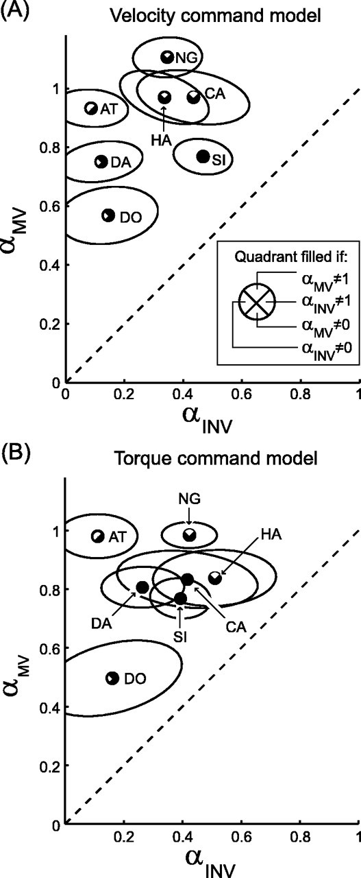
Best-fit values of α_MV and α_INV for all subjects and both models. Each symbol is divided into quadrants that are filled or empty depending on the results of the specified hypothesis tests (p < 0.05; see inset). Ellipses represent 1 SE (bootstrap analysis; see Materials and Methods). Two-letter labels identify individual subjects. The dashed line represents α_INV = α_MV.

The difference between the fit values of the two weighting parameters suggests that the two position estimates x̂_MV and x̂_INV are indeed distinct quantities. We examined this hypothesis by testing whether the fit values of α_MV and α_INV differed significantly from each other (see Materials and Methods). In 12 of 14 cases, the permutation test allowed us to reject the null hypothesis that the two parameters were equal (the exceptions were subjects DO and HA; torque command model). These results were confirmed by an F test (p < 0.05), which agreed with the permutation test in all but a single case (subject CA; torque command model). In the majority of cases, therefore, the two position estimates relied on different combinations of sensory input, reflecting a significant difference between multisensory integration at the two stages of reach planning proposed by our models.

Both the velocity command and torque command models fit the observed data well, and neither performed consistently better across subjects (R² values ranged from 0.63 to 0.80 for the velocity command model and from 0.45 to 0.80 for the torque command model). This similarity suggests that the choice of controlled variable (joint velocities or joint torques) in the model is not critical and that our results follow from the assumption of a two-stage planning process in which a desired extrinsic movement vector is computed and then converted into an intrinsic motor command. Additionally, our assumption that visual and proprioceptive signals are additively combined in Cartesian space (Eqs. 1, 2) did not influence our conclusions. We found nearly identical values of α_MV and α_INV (all absolute differences <0.003) when we refit the data with an alternate model in which visual and proprioceptive cues were combined in joint angle coordinates, implemented by substituting a for each x̂ in Equations 1 and 2.

In our models, the position estimates x̂_MV and x̂_INV are weighted sums of x̂_vis and x̂_prop (Eqs. 1, 2). In other words, we have assumed that each combined position estimate lies on the line that connects the two unimodal estimates and that the distance along that line is determined by the parameter α_MV or α_INV. However, van Beers et al. (1999) have argued that because individual sensory modalities are more or less reliable along different spatial axes, a simple scalar weighting of two unimodal estimates may not produce the statistically optimal combination of these signals. These authors supported their argument by showing that in some conditions the integrated estimate of arm position lies off the straight line connecting the visual and proprioceptive estimates. Such a finding suggests that x̂_MV and x̂_INV might vary across the two-dimensional horizontal plane and that a weighted-sum model might be insufficient. To address this issue, we fit our data with a second alternate model in which x̂_MV and x̂_INV were free to vary across the horizontal plane. Despite this freedom, the best-fit x̂_MV and x̂_INV still lay near the line connecting the unimodal estimates, and there was no consistent component perpendicular to that line (data not shown). Furthermore, the component along the line agreed with the fits shown in Figure 7. These results validate the original weighted-sum model of Equations 1 and 2 for our data. Note, however, that these findings do not necessarily contradict the model of van Beers et al. (1999), because our study was conducted in a different part of the workspace, and workspace location has been shown to influence the orientations of the unimodal covariance ellipses (van Beers et al., 1998).

To fit our models to the data, we have also assumed that the visual and proprioceptive position estimates are unbiased. The analysis described in the preceding paragraph suggests that if any biases exist, they lie principally along the axis parallel to the feedback shift. In fact, such biases could arise for two different reasons. First, the unimodal estimates may be inherently biased, so that x̂_vis and x̂_prop might differ from the locations of the feedback spot and the fingertip, respectively. A second source of bias could arise in the internal transformations of the visual and proprioceptive signals required at each planning stage. For example, comparing x̂_prop with the target location might require computing the Cartesian fingertip location from the proprioceptive signal, whereas evaluating the inverse model might require a joint-based representation. If these transformations were biased, the true value of x̂_prop may not be the same in Equations 1 and 2. In the Appendix, we show that neither of these types of bias would significantly affect the fit values of α_MV and α_INV.

Position-dependent changes in the distortion matrix

The empirical measurements of the direction of the initial velocity and acceleration had to be taken after the onset of the reach, at which point the fingertip had moved a small distance from its initial position. On the other hand, when fitting the models to the data, the model distortion matrices were evaluated at the initial position of the fingertip. This simplification would have a negligible effect if the distortion matrix were nearly constant over the initial movement segment. However, if the distortion matrix varied rapidly across the workspace, there would be a marked change in INV error between the initial arm position and the location at which the velocity and acceleration measurements were made. We assessed whether the assumption of a constant distortion matrix significantly affected our results by determining how the predicted INV error in the velocity command model varies over the initial segment of the trajectory (Fig. 8). For a given arm position, the INV error (that is, the error introduced via the distortion matrix) depends on three variables: the true arm position, the error in the estimated arm position, and the desired movement direction. For this analysis, we assumed that the arm position estimate was equal to the location of the visual feedback (α_INV = 1). This was the conservative choice, because it maximizes the INV error. We also averaged the predicted error over the eight target directions, because the INV error varies little over the desired movement direction (Fig. 4C). We then calculated the predicted INV error for each shift direction as a function of the arm's position for a representative subject and made a contour plot of the results (Fig. 8, gray lines). Superimposed on these plots are the initial segments of the same subject's reach trajectories, ending at the point where the velocity and acceleration were measured. Note that the predicted INV error typically varied <0.5° over the initial movement segment. In contrast, for this subject, the direction of the initial velocity had a within-condition SD of 5.73°. Therefore, any error in model prediction stemming from the assumption of a stationary distortion matrix would be lost in the inherent movement variability.

Figure 8.

Initial reach segments and predicted INV error. The initial portion of reaches (un-filtered empirical data) are shown for all trials from subject HA in the Center-Left (A) and Center-Right (B) conditions. Black lines represent the path from movement onset to the point at which the tangential velocity first exceeds 40% of the peak velocity (black dots). The large circle (dashed line) represents the center start point window (radius 1 cm). Gray contour lines show the magnitude of the predicted INV errors (velocity command model) caused by the distortion matrix as a function of arm position, assuming α_INV = 1. Positive contour values correspond to CCW errors; negative values signify CW errors.

Magnitude of initial velocity

In our models, α_MV and α_INV were fit using only the directional component of the error in initial reach velocity or acceleration. Here, we show that the shifts in visual feedback also lead to errors in the magnitude of the initial velocity and that these errors are consistent with the predictions of the velocity command model. The results for initial acceleration and the torque command model are qualitatively the same.

First consider that both the direction and magnitude of the INV velocity error are determined by the distortion matrix, , as shown in Equation 5. For the starting location and visual shift directions used in this experiment, the distortion matrices are mostly rotational, i.e., the desired velocity undergoes a rotation but very little scaling. We determined this by evaluating the velocity distortion matrix at the starting location for each subject for both the left and right visual shifts using the best-fit α_INV. We then found the velocity direction that yielded the greatest absolute percentage change in the magnitude of the velocity. Across subjects and shift directions, the average maximum scaling was only 0.75 ± 0.44% (mean ± 1 SD) of the original length. The model therefore predicts that in our experiment the INV error should have a negligible effect on the magnitude of the velocity.

In contrast, MV error alters both the direction and length of the planned movement vector, and we would expect these variables to influence the magnitude of the planned velocity. This effect can be understood by considering the movements made from the left and right start points in the absence of a visual shift. For each subject and target, the peak velocities for reaches in the Left-Zero and Right-Zero conditions were normalized to the average peak velocity for the same target in the Center-Zero condition. These values are plotted as a function of target direction in Figure 9 (filled symbols). This is the pattern that would be expected in the Center-Left and Center-Right conditions if the estimated arm positions were located at the left and right starting locations, respectively (i.e., if α_MV = 1). If there were no error in the position estimate (α_MV = 0), the average peak velocity would be the same as in the Center-Zero condition, and so the normalized values would all be near unity. As can be seen from the open symbols in Figure 9, the dependence of peak velocity on target direction in the Center-Left and Center-Right trials has the same shape as that seen in the Left-Zero and Right-Zero conditions, but the effect is smaller in size. Qualitatively, this is the pattern of MV errors that the velocity command model would predict for the best-fit values of α_MV, which are less than 1.

Figure 9.

Effects of visual shifts on reach velocity magnitude. Each line plots the mean peak tangential velocity (across subjects) for each target normalized to the mean peak tangential velocity in Center-Zero trials. Target directions are defined as the direction from the fingertip start position to the visual target. A, Left-Zero (solid line) and Center-Left (dotted line) trials. B, Right-Zero (solid line) and Center-Right (dotted line) trials. Error bars are ± 1 SE.

Discussion

By dissociating visual and proprioceptive feedback, we induced errors in the arm position estimates used at two different stages of reach planning. We then modeled the errors in initial movement direction as a function of the misestimation at each stage. Comparison of our models with the experimental data allowed us to quantify these position errors and thus compute the extent to which each planning stage relies on visual feedback. We found that the arm position estimate used for vector planning relies mostly on visual feedback, whereas the estimate used to convert the desired movement vector into a motor command relies more on proprioceptive signals.

This finding agrees with the results of a recent study by Sainburg and colleagues (2003) that employed a reaching task very similar to our own. In their experiment, the location of the initial visual feedback was constant across trials whereas the actual initial location of the fingertip was varied. The authors found that these manipulations did not affect reach direction, suggesting that subjects relied heavily on the visual position signal (which did not change location) when planning movement vectors. Furthermore, an inverse dynamic analysis revealed that subjects generated intrinsic motor commands that took into account the true position of the arm, suggesting that subjects relied mostly on proprioceptive signals when generating motor commands. Although the relative weightings of vision and proprioception were not quantified, these results are in agreement with our own.

Psychophysical studies of the tradeoff between vision and proprioception in arm position estimation have suggested that each modality is weighted according to its statistical reliability (Howard and Templeton, 1966; Welch and Warren, 1980; van Beers et al., 1999) or depending on the focus of the subject's attention (Warren and Schmitt, 1978; Welch and Warren, 1980). However, although both of these factors may influence multisensory integration, these models provide only a single criterion for weighting the unimodal signals. Such models cannot account for our finding that vision and proprioception are weighted differently at different stages of motor planning.

Our results instead suggest that multisensory integration depends on the computations in which the integrated estimates are used. To compute the movement vector, for example, the position of the hand must be compared with that of the target in a common coordinate frame. Transforming signals from one coordinate frame to another presumably incurs errors, either from imperfections in the mapping between them (bias) or because of noise introduced in the additional computation (variance). The effects of these errors on movement control can be reduced by giving less weight to transformed signals. In our experiment, where targets are presented visually, the increased reliance on visual feedback when planning movement vectors therefore would have been advantageous.

A similar argument can explain the predominance of proprioception when transforming the movement vector into a motor command. Computing the inverse model of the arm requires knowledge of the arm's posture. Although our experimental constraints created a one-to-one relationship between joint angles and fingertip location, during more natural, unconstrained movements joint angles cannot be uniquely inferred from visual feedback specifying only the location of the fingertip. Additionally, errors can arise from biases in the coordinate transformation from extrinsic to intrinsic coordinates (Soechting and Flanders, 1989) and from variance introduced during the computation, as in the first stage of planning. Because of these factors, the reduced reliance on vision at this second planning stage would have been advantageous.

This interpretation is compatible with a modified minimum-variance principle that takes into account the errors introduced by coordinate transformations. The computations performed at each stage require information about different aspects of the position of the arm: when reaching to a visual target, movement vector planning requires only the extrinsic location of the fingertip, whereas computing the inverse model of the arm requires knowing the intrinsic, joint-based posture of the arm. The values of α_MV and α_INV reflect this difference, because the nervous system relies more heavily on the signals that contain the information necessary to perform the relevant computation and do not need to be transformed.

These conclusions are made primarily on the basis of the analyses of initial movement direction. However, numerous authors have argued that the planning of reach direction and extent are independent processes (Gordon et al., 1994a; Messier and Kalaska, 1997). If this hypothesis were true, the rules for integrating vision and proprioception might be different for the planning of movement extent and direction. Indeed, such a difference was found in the recent study by Sainburg and colleagues (2003). As noted above, they found that the direction of movements to a given target depended on the location of the visual feedback and not on the actual position of the arm. In contrast, planning of movement extent appeared to depend on the arm's true position to a greater or lesser degree, depending on the position of the arm relative to the target. Our results do not rule out the possibility that a separate estimate or set of estimates is used to compute movement extent. Nonetheless, we have shown in Figure 9 that the peak velocity relies on a position estimate located between the positions specified by vision and proprioception, consistent with the results of our analyses of movement direction. Although these data suggest that the planning of reach amplitude and direction might use the same position estimates, this hypothesis would have to be confirmed by a study that better controlled for the various factors affecting reach amplitude.

Our quantification of sensory integration relies on model-based analyses of the empirical data. We therefore must address how sensitive our conclusions are to the details of the model. First, the velocity command and torque command models produce similar estimates of multisensory integration at each planning stage (Fig. 7). This shows that our results do not depend critically on the assumption that the nervous system specifies kinematic or dynamic motor commands. Second, the alternate model in which the two signals are combined in intrinsic space produces the same fit values, showing that our results are not sensitive to the assumption that unimodal signals are additively combined in extrinsic space. Third, the alternate model in which α_MV and α_INV were allowed to vary across the horizontal plane produces results similar to those of the one-dimensional models, demonstrating that our results do not depend on the assumption that vision and proprioception are weighted by a scalar term.

Despite these invariances, however, all of our models make the basic assumption that motor planning involves two stages, each using a separate estimate of arm position. This need not be the case, because in theory the whole planning process could be done in a single computational stage that computes an intrinsic motor command directly from the target location and a single estimate of the initial arm position (Uno et al., 1989). However, even if motor planning were performed in a single stage, the two types of error described in this paper would still arise. A single-stage planner receiving unshifted feedback from the arm would determine the motor command appropriate to move the hand from the initial position to the target. The resulting movement constitutes the baseline trajectory. If the arm position estimate is shifted, the motor command will be the one appropriate to move the arm from the incorrect estimated location to the target. This command would achieve the target location if the arm were actually at the estimated position, and we will refer to that hypothetical trajectory as the planned trajectory. The difference between the planned and baseline trajectories is essentially the MV error described above. Because the arm is not at the estimated location, however, when the motor command is executed, the resulting reach direction will differ from that of the planned trajectory. This difference is the INV error. If such a single-stage planner were in fact in operation, the MV and INV errors would be attributable to a single shifted estimate of arm position, and so we would expect that our analyses would find equal values for α_MV and α_INV. The fact that we found consistent differences between α_MV and α_INV suggests that planning indeed involves two separate stages.

Many cortical areas that encode pending movements appear to integrate information from multiple sensory modalities (Colby and Duhamel, 1996; Andersen et al., 1997; Wise et al., 1997), and single cortical neurons encoding arm position show varying weightings of visual and proprioceptive feedback from the arm (Graziano, 1999; Graziano et al., 2000). Given these findings, it is tempting to speculate that the two planning stages proposed in this paper might be computed in different cortical areas. Two lines of evidence support the idea that the parietal cortex is involved in the computation of extrinsic movement vectors. Recordings from the intraparietal sulcus have revealed coding of reach direction in retinocentric coordinates (Buneo et al., 2002), suggesting that this area encodes movement vectors but not intrinsic motor commands. Additionally, disruption of neural activity in the posterior parietal cortex by transcranial magnetic stimulation prevents subjects from making corrective movements during reaching (Desmurget et al., 1999), providing further evidence that this region might help compute the discrepancy between hand position and target location. Studies examining the motor and premotor cortices, on the other hand, suggest a role for these areas in transforming movement vectors into motor commands. Neural activity in these areas during both single- and multi-jointed movements encodes the intrinsic details of the movement in addition to the extrinsic movement vector (Scott and Kalaska, 1997; Scott et al., 1997; Kakei et al., 1999). However, these findings do not represent a complete dissociation between parietal and frontal cortices. For example, Scott et al. (1997) showed that activity in parietal area 5 is also modulated by intrinsic factors. Future studies that use manipulations of sensory feedback to selectively alter the extrinsic movement vector and intrinsic motor commands will be needed to clarify the neural bases of these two computations.

Appendix

As described in Materials and Methods, in determining the weighting parameters α_MV and α_INV we assumed that the unimodal position estimates x̂_vis and x̂_prop were unbiased. In this Appendix, we consider the effects of biases in the unimodal position signals on the fit values for the α_MV and α_INV. We will show that sensory biases along the direction of the visual shift (Fig. 1, 0°) would not bias our fit values for α_MV and α_INV.

Given values for the unimodal positions estimates, an integrated position estimate x̂ (which could be either x̂_MV or x̂_INV) can be computed from the appropriate weighting parameter α (α_MV or α_INV), and vice versa:

11

12

Note that in contrast to Materials and Methods, in Equation 12 and the rest of this Appendix we treat all position and bias variables as scalar values along the 0° axis. Because we do not have direct access to the internal unimodal estimates x̂_vis and x̂_prop, we previously assumed that these estimates were unbiased, i.e., that x̂_prop = x, the true location of the arm, and that x̂_vis was offset from that location by the visual shift. Here, we consider the possibility that the unimodal estimates are biased by amounts b_prop and b_vis, respectively:

where the visual shift is -Δ in Center-Left trials and +Δ in Center-Right trials.

We first explore how these biases would affect our estimates of α when fit separately to trials with left and right visual shifts. Consider dividing our data into two sets, one containing Center-Left and Center-Zero trials and the other containing Center-Right and Center-Zero trials. The integrated position estimates and the best-fit weighting parameters pertaining to the two datasets will be identified by the subscripts L and R. Given values for the unimodal biases, the integrated position estimates can be determined from the true weighting parameter α and Equation 11:

13

14

If α_L were fit with the assumption that b_prop = b_vis = 0, we would still be able to obtain the true value for x̂_L by evaluating Equation 13 with b_prop = b_vis = 0 and the fit value of α_L. Counterintuitively, this means that we would be able to recover the true value of x̂_L even from a biased fit value for α_L. Next, we can determine the bias in our fit value of α_L by inserting the true value of x̂_L (Eq. 13) into a version of Equation 12 that assumes, as do our models, that x̂_vis and x̂_prop are unbiased:

15

Similarly, from the Center-Right trials and Equations 12 and 14 we would find:

16

Equations 15 and 16 suggest that the presence of biases in the internal unimodal position estimates would cause errors in our fit values of α_MV and α_INV. However, a comparison of these two equations shows that the effects on the Center-Left and Center-Right trials are in the opposite direction, as long as the bias terms do not depend on the trial condition (a reasonable assumption given that the trials are interleaved and that the proprioceptive location, at least, is constant across trials). Therefore, in the complete analysis in which α_MV and α_INV are fit to all trials, we expect that any bias effects would cancel out.

This observation can be made more rigorous by averaging Equations 15 and 16, giving:

17

Equation 17 tells us that the average of the parameters fit to the R and L datasets should be equal to the true weighting parameters, regardless of potential biases in the unimodal position signals. For each subject and each model, we fit α_MV and α_INV to the R and L datasets, and then compared (α_L + α_R)/2 with the fit values of α shown in Figure 7. The mean ± SD difference is 0.0067 ± 0.017, with a maximum absolute difference of 0.068. These results show that our assumption of unbiased unimodal signals had a negligible effect on our results. Additionally, note that because these arguments can be applied separately to the parameters α_MV and α_INV, Equation 17 holds for both parameters even if the biases in a unimodal position estimate are different between Equations 1 and 2. For this reason, biases in the transformations between coordinate frames (see Results) cannot be responsible for our findings.

References

- Aglioti S, DeSouza JFX, Goodale MA ( 1995) Size-contrast illusions deceive the eye but not the hand. Curr Biol 5: 679-685. [DOI] [PubMed] [Google Scholar]
- Andersen RA, Snyder LH, Bradley DC, Xing J ( 1997) Multimodal representation of space in the posterior parietal cortex and its use in planning movements. Ann Rev Neurosci 20: 303-330. [DOI] [PubMed] [Google Scholar]
- Atkeson CG, Hollerbach JM ( 1985) Kinematic features of unrestrained vertical arm movements. J Neurosci 5: 2318-2330. [DOI] [PMC free article] [PubMed] [Google Scholar]
- Buneo CA, Jarvis MR, Batista AP, Andersen RA ( 2002) Direct visuomotor transformations for reaching. Nature 416: 632-636. [DOI] [PubMed] [Google Scholar]
- Cheney PD, Fetz EE ( 1980) Functional classes of primate corticomotoneuronal cells and their relation to active force. J Neurophysiol 44: 773-791. [DOI] [PubMed] [Google Scholar]
- Colby CL, Duhamel JR ( 1996) Spatial representations for action in parietal cortex. Cognit Brain Res 5: 105-115. [DOI] [PubMed] [Google Scholar]
- Desmurget M, Epstein CM, Turner RS, Prablanc C, Alexander GE, Grafton ST ( 1999) Role of the posterior parietal cortex in updating reaching movements to a visual target. Nat Neurosci 2: 563-567. [DOI] [PubMed] [Google Scholar]
- Draper N, Smith H ( 1998) Applied regression analysis, Ed 3. New York: Wiley.
- Efron B, Tibshirani RJ ( 1993) An introduction to the bootstrap. Boca Raton, FL: Chapman and Hall.
- Ernst MO, Banks MS ( 2002) Humans integrate visual and haptic information in a statistically optimal fashion. Nature 415: 429-433. [DOI] [PubMed] [Google Scholar]
- Flash T, Hogan N ( 1985) The coordination of arm movements: an experimentally confirmed mathematical model. J Neurosci 5: 1688-1703. [DOI] [PMC free article] [PubMed] [Google Scholar]
- Georgopoulos AP, Kalaska JF, Caminiti R, Massey JT ( 1982) On the relations between the direction of two-dimensional arm movements and cell discharge in primate motor cortex. J Neurosci 2: 1527-1537. [DOI] [PMC free article] [PubMed] [Google Scholar]
- Ghahramani Z ( 1995) Computation and psychophysics of sensorimotor integration. PhD Thesis, Massachusetts Institute of Technology.
- Ghilardi MF, Gordon J, Ghez C ( 1995) Learning a visuomotor transformation in a local area of work space produces directional biases in other areas. J Neurophysiol 73: 2535-2539. [DOI] [PubMed] [Google Scholar]
- Good P ( 2000) Permutation tests. Springer Series in Statistics, Ed 2. New York: Springer-Verlag.
- Goodale MA, Milner AD ( 1992) Separate visual pathways for perception and action. Trends Neurosci 15: 20-25. [DOI] [PubMed] [Google Scholar]
- Goodbody SJ, Wolpert DM ( 1999) The effect of visuomotor displacements on arm movement paths. Exp Brain Res 127: 213-223. [DOI] [PubMed] [Google Scholar]
- Gordon J, Ghilardi MF, Ghez C ( 1994a) Accuracy of planar reaching movements. I. Independence of direction and extent variability. Exp Brain Res 99: 97-111. [DOI] [PubMed] [Google Scholar]
- Gordon J, Ghilardi MF, Cooper SE, Ghez C ( 1994b) Accuracy of planar reaching movements. II. Systematic extent errors resulting from inertial anisotropy. Exp Brain Res 99: 112-130. [DOI] [PubMed] [Google Scholar]
- Graziano MSA ( 1999) Where is my arm? The relative role of vision and proprioception in the neuronal representation of limb position. Proc Natl Acad Sci USA 96: 10418-10421. [DOI] [PMC free article] [PubMed] [Google Scholar]
- Graziano MSA, Cooke DF, Taylor CSR ( 2000) Coding the location of the arm by sight. Science 290: 1782-1786. [DOI] [PubMed] [Google Scholar]
- Haffenden AM, Schiff KC, Goodale MA ( 2001) The dissociation between perception and action in the Ebbinghaus illusion: nonillusory effects of pictorial cues on grasp. Curr Biol 11: 177-181. [DOI] [PubMed] [Google Scholar]
- Howard IP, Templeton WB ( 1966) Human spatial orientation. London: Wiley.
- Jacobs RA ( 1999) Optimal integration of texture and motion cues to depth. Vision Res 39: 3621-3629. [DOI] [PubMed] [Google Scholar]
- Jordan MI ( 1996) Computational aspects of motor control and motor learning. In: Handbook of perception and action: motor skills (Heuer H, Keele S, eds), pp 71-120. New York: Academic.
- Kakei S, Hoffman DS, Strick PL ( 1999) Muscle and movement representations in the primary motor cortex. Science 285: 2136-2139. [DOI] [PubMed] [Google Scholar]
- Messier J, Kalaska J ( 1997) Differential effect of task conditions on errors of direction and extent of reaching movements. Exp Brain Res 115: 469-478. [DOI] [PubMed] [Google Scholar]
- Milner AD, Goodale MA ( 1995) The visual brain in action. Oxford Psychology Series. Oxford: Oxford UP.
- Paillard J ( 1996) Fast and slow feedback loops for the visual correction of spatial errors in a pointing task: a reappraisal. Can J Physiol Pharmacol 74: 401-417. [PubMed] [Google Scholar]
- Prablanc C, Martin O ( 1992) Automatic control during hand reaching at undetected 2-dimensional target displacements. J Neurophysiol 67: 455-469. [DOI] [PubMed] [Google Scholar]
- Rossetti Y, Desmurget M, Prablanc C ( 1995) Vectorial coding of movement: vision, proprioception, or both? J Neurophysiol 74: 457-463. [DOI] [PubMed] [Google Scholar]
- Sabes PN, Jordan MI ( 1997) Obstacle avoidance and a perturbation sensitivity model for motor planning. J Neurosci 17: 7119-7128. [DOI] [PMC free article] [PubMed] [Google Scholar]
- Sainburg RL, Lateiner JE, Latash ML, Bagesteiro BL ( 2003) Effects of altering initial position on movement direction and extent. J Neurophysiol 89: 401-415. [DOI] [PMC free article] [PubMed] [Google Scholar]
- Scott SH, Kalaska JF ( 1997) Reaching movements with similar hand paths but different arm orientations. I. Activity of individual cells in motor cortex. J Neurophysiol 77: 826-852. [DOI] [PubMed] [Google Scholar]
- Scott SH, Sergio LE, Kalaska JF ( 1997) Reaching movements with similar hand paths but different arm orientations. II. Activity of individual cells in dorsal premotor cortex and parietal area 5. J Neurophysiol 78: 2413-2426. [DOI] [PubMed] [Google Scholar]
- Soechting JF, Flanders M ( 1989) Errors in pointing are due to approximations in sensorimotor transformations. J Neurophysiol 62: 595-608. [DOI] [PubMed] [Google Scholar]
- Soechting JF, Lacquaniti F ( 1981) Invariant characteristics of a pointing movement in man. J Neurosci 1: 710-720. [DOI] [PMC free article] [PubMed] [Google Scholar]
- Todorov E ( 2000) Direct cortical control of muscle activation in voluntary arm movements: a model. Nat Neurosci 3: 391-398. [DOI] [PubMed] [Google Scholar]
- Uno Y, Kawato M, Suzuki R ( 1989) Formation and control of optimal trajectory in human multijoint arm movement: minimum torque-change model. Biol Cybern 61: 89-101. [DOI] [PubMed] [Google Scholar]
- van Beers RJ, Sittig AC, van der Gon JJD ( 1998) The precision of proprioceptive position sense. Exp Brain Res 122: 367-377. [DOI] [PubMed] [Google Scholar]
- van Beers RJ, Sittig AC, van der Gon JJD ( 1999) Integration of proprioceptive and visual position-information: an experimentally supported model. J Neurophysiol 81: 1355-1364. [DOI] [PubMed] [Google Scholar]
- Warren DH, Schmitt TL ( 1978) On plasticity of visual-proprioceptive bias effects. J Exp Psychol Hum Percept Performance 4: 302-310. [DOI] [PubMed] [Google Scholar]
- Welch RB, Warren DH ( 1980) Immediate perceptual response to intersensory discrepancy. Psychol Bull 88: 638-667. [PubMed] [Google Scholar]
- Welch RB, Widawski MH, Harrington J, Warren DH ( 1979) Examination of the relationship between visual capture and prism adaptation. Percept Psychophys 25: 126-132. [DOI] [PubMed] [Google Scholar]
- Wise SP, Boussaoud D, Johnson PB, Caminiti R ( 1997) Premotor and parietal cortex: corticocortical connectivity and combinatorial computations. Annu Rev Neurosci 20: 25-42. [DOI] [PubMed] [Google Scholar]