Temporal Resolution of Ensemble Visual Motion Signals in Primate Retina

Abstract

Recent studies have examined the temporal precision of spiking in visual system neurons, but less is known about the time scale that is relevant for behaviorally important visual computations. We examined how spatiotemporal patterns of spikes in ensembles of primate retinal ganglion cells convey information about visual motion to the brain. The direction of motion of a bar was estimated by comparing the timing of responses in ensembles of parasol (magnocellular-projecting) retinal ganglion cells recorded simultaneously, using a cross-correlation approach similar to standard models of motion sensing. To identify the temporal resolution of motion signals, spike trains were low-pass filtered before estimating the direction of motion. The filter time constant that resulted in most accurate motion sensing was in the range of 10-50 msec for a range of stimulus speeds and contrasts and approached a lower limit of ∼10 msec at high speeds and contrasts. This time constant was, on average, comparable to the length of interspike intervals. These findings suggest that cortical neurons could filter their inputs on a time scale of tens of milliseconds, rather than relying on the precise times of individual input spikes, to sense motion most reliably.

Introduction

Ensembles of neurons encode information in spatiotemporal patterns of spikes. A fundamental aspect of this encoding is its temporal resolution (Bialek et al., 1991; de Ruyter van Steveninck et al., 1997; Rieke et al., 1997). Recent studies have shown that mammalian retinal ganglion cells (RGCs) and lateral geniculate nucleus neurons can exhibit spike timing reproducibility approaching 1 msec in response to repeated stimulation (Berry et al., 1997; Reich et al., 1997; Reinagel and Reid, 2000; Liu et al., 2001). These findings contrast with integration times of tens of milliseconds for mammalian cones (Kraft, 1988; Schnapf et al., 1990), and suggest that the detailed timing of spikes is an essential aspect of visual signaling. However, spike timing precision varies widely with stimulus conditions, and spike trains are often sparse and unreliable. As a result, many visual tasks may demand integration over time to obtain accurate signals, particularly when responses from multiple neurons must be compared. Thus, it is unclear whether the extremes of precision observed in individual neurons reveal the time scale most relevant for behaviorally important computations in populations of neurons.

Here we develop an approach to determine the time scale relevant for sensing the direction of visual motion. Motion sensing is an important test case because it is behaviorally significant and relies entirely on the temporal pattern of spikes in a population of neurons. Primate RGCs that transmit visual information to the cortex via the magnocellular layers of the lateral geniculate nucleus are not individually selective for the direction of motion; instead, motion is represented in the spatiotemporal pattern of activity in many RGCs. Thus, direction-selective cortical neurons must compare the timing of spikes from multiple non-direction-selective inputs to sense motion. For this comparison to be reliable, it must be performed at a temporal resolution matched to input spiking statistics. If moving stimuli induce spike trains in nearby RGCs that are precisely and reliably timed relative to one another, cortical neurons could extract the highest-fidelity representation of visual motion by comparing the arrival times of spikes from different inputs at fine temporal resolution. Conversely, if RGC spike trains induced by moving stimuli are not precisely and reliably timed relative to one another, cortical neurons could most accurately sense motion by discarding fine temporal structure and comparing the timing of their inputs at a coarser resolution. These considerations suggest that there is an optimal temporal resolution for reading out ensemble visual motion signals in RGCs.

Because the activity of nearby RGCs is not statistically independent (Mastronarde, 1983; Meister et al., 1995), the readout of retinal motion signals can only be examined accurately using simultaneous recordings from multiple cells. Using multielectrode recordings from the primate retina, we examined responses elicited by moving bars in collections of parasol RGCs, which convey motion information to the brain. The direction of stimulus motion was extracted from this ensemble activity using a cross-correlation approach similar to standard models of motion sensing. We examined how the temporal resolution of motion readout influences the accuracy of direction discrimination by filtering RGC spike trains before cross-correlating. Accuracy was low for readout performed with very coarse (100 msec) and very fine (1 msec) filtering, and optimal readout was obtained by filtering on a time scale of 10-50 msec for a range of stimulus speeds and contrasts. This provides a measure of the temporal resolution of early visual motion signals and suggests the temporal filtering of retinal inputs that might be expected in direction-sensing circuits in the brain.

Materials and Methods

Recordings. Eyes were obtained from terminally anesthetized macaque monkeys (Macaca mulatta; Macaca radiata) used by other experimenters, in accordance with institutional guidelines for the care and use of animals. Immediately after enucleation, the anterior portion of the eye and vitreous were removed in room light, and the eye cup was placed in bicarbonate-buffered Ames solution (Sigma, St. Louis, MO) and stored in darkness for at least 20 min before dissection. Under infrared illumination, pieces of retina 2-4 mm in diameter were cut from regions 20-50° from the fovea and placed flat against a planar array of 61 extracellular microelectrodes that were used to record action potentials from retinal ganglion cells (Meister et al., 1994; Chichilnisky and Baylor, 1999b). The preparation was perfused with Ames solution bubbled with 95% O₂ and 5% CO₂ and maintained at 34-36°C, pH 7.4. In the first experiment, the retinal pigment epithelium (RPE) was left attached to the retina. In the second and third experiments, the RPE was separated from the retina before recording. In what follows, when data from different preparations are described separately, they are presented in the same order as above.

Retinal eccentricity was measured with a precision of 1-2 mm. Eccentricity was converted to a temporal equivalent value, because the contours of constant RGC density (and thus presumably dendritic- and receptive field size) in the macaque monkey retina are approximately semicircular in the temporal half of the retina, but elliptical with an aspect ratio of 0.61 in the nasal half (Perry and Cowey, 1985; Watanabe and Rodieck, 1989). Thus, a location X mm nasal and Y mm superior (or inferior) to the fovea was assigned an equivalent eccentricity of . A location X mm temporal and Y mm superior (or inferior) to the fovea was assigned an equivalent eccentricity of . Visual angle (A) in degrees was computed from temporal equivalent eccentricity (E) in millimeters using the following relation: A = 0.1 + 4.21 E + 0.038 E² (Perry and Cowey, 1985; Dacey and Petersen, 1992). The temporal equivalent eccentricities (visual angles) of the three preparations recorded were 9.5 mm (44°), 6.1 mm (27°), and 4.7 mm (21°), respectively.

Spikes were digitized at 20 kHz (Meister et al., 1994; Litke, 1999) and stored for off-line analysis. Spikes from different cells were segregated by identifying distinct clusters of spike height and width recorded on each electrode and verifying the presence of a refractory period. Maintained firing rate (mean ± SD across all of the ON and OFF cells) during exposure to spatially uniform background light (see below) was 14 ± 5, 7 ± 6, and 4 ± 4 Hz in each of the three preparations, respectively.

Stimuli. The preparation was stimulated with the optically reduced (1.3 mm diameter) image of a cathode ray tube (CRT) computer display refreshing at 120 Hz, focused on the photoreceptor layer by a microscope objective, and centered on the 480 μm-diameter electrode array. Stimuli were attenuated to low photopic light levels using neutral-density filters. In isolated retina experiments, the stimulus was delivered from the photoreceptor side. In experiments in which the RPE was attached, the retina was stimulated from the ganglion cell side through the mostly transparent electrode array. In the latter case, the shadows cast by the platinized (black) electrode tips (5 μm in diameter and spaced 60 μm apart) had a minimal influence on the intensity or spatial pattern of the stimulus, because they occupied ∼1% of the total area of the array and were optically diffused by virtue of lying in a different focal plane than the photoreceptors.

All stimuli were presented as modulations around a mean gray background. The background photon absorption rates for the long-, middle-, and short-wavelength-sensitive cones were approximately equal to the absorptions that would have been caused by spatially uniform monochromatic lights of 561, 530, and 430 nm wavelength and 9000, 9000, and 5000 photons · μm^-2 · sec^-1 intensity, respectively, incident on the photoreceptors.

RGCs were characterized and classified on the basis of their responses to a white-noise stimulus presented for 15-30 min (Sakai et al., 1988; Chichilnisky, 2001). The stimulus was a square lattice of randomly flickering pixels. Random flicker was created by selecting the intensities of the red, green, and blue display phosphors at each pixel location independently from a Gaussian or binary (two-valued) distribution on each stimulus frame. This stimulus modulated photon absorptions asynchronously in all three cone types. The light response properties of each cell were summarized by the average stimulus on the display over 250 msec preceding a spike [spike-triggered average (STA)]. The STA is a measure of how effectively stimuli at different locations and with different colors are integrated by the cell over time to control firing. The structure of each receptive field was measured by fitting the STA with a difference of elliptical Gaussians (center-surround) spatial profile, a difference of low-pass filters temporal profile, and a relative sensitivity to modulation of each phosphor. The product of these terms provided accurate fits to the space-time-color STA (Chichilnisky and Kalmar, 2002).

Analysis of responses to moving stimuli was restricted to a class of commonly recorded cells whose receptive field tiling and density, spectral sensitivity, response kinetics, and contrast gain obtained from the STA were consistent with those of the anatomically defined parasol cells of the retina of the macaque (Chichilnisky and Kalmar, 2002). Visual inspection of rasters of repeated responses to moving bars was used to exclude a minority of cells whose responses were unstable or obviously differed from those of other putative parasol cells simultaneously recorded, to avoid artificially coarse estimates of temporal resolution.

Moving bars of different positive and negative contrasts and speeds were presented in randomly interleaved trials. The bar length (orthogonal to direction of motion) covered the entire area recorded and the bar width (parallel to direction of motion) was 118 μm. For comparison, the mean receptive field diameter for the putative parasol cells recorded in each of the three preparations was 164, 96, and 100 μm, respectively. Receptive field diameter was defined as the geometric mean of the major and minor axes of the 1 SD boundary of the center Gaussian fit to the STA spatial profile (see above) (Chichilnisky and Kalmar, 2002). The rasterization of the CRT display introduced a space-time sampled representation of the moving bar. For example, a bar nominally moving at 29.4 deg · sec^-1 was in fact redrawn on the CRT every 8.33 msec, displaced by 49 μm (stimulus dimensions were converted to degrees using the approximation 200 μm · deg^-1 for the peripheral primate retina) (Perry and Cowey, 1985). Speeds of >60 deg · sec^-1 were not probed, because they would have resulted in displacements greater than the width of the bar.

Data from three preparations are presented in Results, with cells, speeds, contrasts, and number of trials as follows: retina 1, 6 ON, 4 OFF; speeds, 14.7, 29.4, and 58.7 deg · sec^-1; contrasts, ±96%; 80 trials; retina 2, 6 ON, 14 OFF; speeds 3.6, 7.1, 14.2, and 28.4 deg · sec^-1; contrasts, ±12, 24, 48, and 96%; 50 trials; retina 3, 11 ON, 5 OFF; speeds, 3.6, 7.1, 14.2, and 35.5 deg · sec^-1; contrasts, ±12, 24, 48, and 96%; 20 trials.

Analysis. In each trial, the temporal pattern of responses from multiple RGCs was used to compute a net motion signal. The sign of the net motion signal provided an estimate of the direction of motion of the bar from the spike trains. The net motion signal was computed as follows. Let s_A(t) and s_B(t) represent the spike counts as a function of time recorded from cells A and B, respectively, represented in bins of size 0.05 msec (see Fig. 2). These responses were convolved with a low-pass filter to create filtered responses, r_A(t) = s_A(t) * f(t) and r_B(t) = s_B(t) * f(t), where f(t) = e^-t/τ for t ≥ 0 and f(t) = 0 for t < 0 (see Fig. 2), and represented using bins of size . The filter width, or time constant τ, was varied (see Fig. 4). In some cases, a Gaussian filter g(t) = e^-t2/2σ² was used, and the value of σ was varied. A signal indicative of rightward motion was obtained by delaying the filtered response of cell A by an amount Δt, multiplying pointwise by the filtered response of cell B, and summing the result: R = Σ_tr_A(t - Δt)r_B(t), where the summation is over all of the time points in the trial, and r_A(t -Δt) is circularly shifted to match the duration of r_B(t). The delay value Δt was the bar speed divided by the distance along the axis of motion between the midpoints of the receptive fields of the two cells (these midpoints were obtained using parametric fits to the STA) (Chichilnisky and Kalmar, 2002). A signal indicative of leftward motion was created symmetrically: L =Σ_tr_B(t -Δt)r_A(t). The net motion signal N for this cell pair was given by the difference, N = R - L. The net motion signal for a collection of cells was the sum of the net motion signals obtained from all of the distinct pairs; ON and OFF populations were considered separately because of their different response kinetics (Chichilnisky and Kalmar, 2002). On average, rightward-moving bars yielded positive net motion signals, and leftward-moving bars yielded negative net motion signals, as expected (see Fig. 3).

Figure 2.

Opponent detector for motion readout. The procedure for reading out the direction of motion from ensemble RGC activity is depicted schematically, operating on hypothetical spike trains (black vertical ticks) obtained from two cells in response to a bar moving from left to right. Each spike train is low-pass filtered in time (gray smooth traces superimposed on spike trains). For a rightward detector, the filtered response from cell A is delayed by a fixed amount and multiplied pointwise by the filtered response from cell B. The result is summed over time to yield a rightward motion signal. A leftward motion signal is obtained by delaying the response from cell B instead. The difference between rightward and leftward motion signals is the net signal used to estimate the direction of motion. In the case shown, the rightward motion signal is larger than the leftward motion signal, so the net motion signal is positive.

Figure 4.

Dependence of the SNR on temporal filtering. SNR is shown as a function of filter width (time constant) for three stimulus speeds (shown inset) in one preparation. SNR was computed from the pooled distribution of net motion signals obtained in trials with leftward and rightward motion, with the sign of the signal on leftward trials inverted. A, Six ON cells (bar contrast, 96%). B, Four OFF cells (bar contrast, -96%).

Figure 3.

Net motion signals for moving bars. A, Net motion signals obtained from six ON cells in response to 80 trials of a leftward (rightward)-moving bar are shown in the histogram on the left (right). Filter time constant (τ), 1 msec; bar contrast, 96%; bar speed, 29.4 deg·sec^-1. The SNR is shown inset. B, Same data, but filtered with a time constant of 10 msec. C, Same data, but filtered with a time constant of 100 msec. Because the units on net motion signals are arbitrary, the values in each histogram were normalized to unit mean.

Motion detectors were constructed with an explicit delay, although delay lines have not been observed in the mammalian visual system (but see Mastronarde et al., 1991). A common alternative approach—using coarse temporal filtering to approximate a delay—may more closely resemble biological motion sensing. However, in the latter approach, temporal resolution (see Results) is confounded with speed tuning, because both are controlled by filter width.

The pairwise computation of the net motion signal described above is equivalent to an approach that combines responses of all of the cells simultaneously. For the ith cell, let Δt_i represent the time required for a rightward-moving bar to move from the midpoint of the receptive field of the cell to a fixed, arbitrary reference location. In the case of rightward motion, the right-delayed responses r_i(t - Δt_i) (circularly shifted, as above) from all of the cells should be approximately aligned, and the left-delayed responses r_i(t + Δt_i) should be misaligned. Thus, the degree of alignment of all of the right-delayed (left-delayed) responses indicates the evidence for rightward (leftward) motion. A measure of alignment can be obtained by adding all of the responses pointwise and summing the squared entries of the result: the squaring operation provides a greater signal when the various responses are aligned. This yields rightward and leftward motion signals:

1

2

3

4

Because summation is over all of the times t and delayed responses are circularly shifted, the first terms in R and L are equal. This leaves the difference N consisting of the remaining cross terms, which is exactly twice the motion signal obtained from the summed pairwise product of delayed spike trains used above. Thus, the pairwise motion sensing algorithm is equivalent to an algorithm that integrates responses of all of the cells simultaneously.

Motion sensing algorithms can also be defined on the basis of other measures of response alignment. One approach evaluated in Results is based on principal components analysis. The fraction of the variance of a collection of responses explained by the first principal component defines an index of alignment. If the index is 1, then all of the responses differ by at most a scale factor. If the index is small, then the response waveforms differ. The index of alignment was obtained by creating a matrix composed of one row for the response of each cell, computing the singular value decomposition of this matrix, and dividing the square of the first singular value by the sum of the squares of all of the singular values. The net motion signal was defined as the difference between the index of alignment obtained from right-delayed responses, r_i(t - Δt_i), and left-delayed responses, r_i(t + Δt_i).

Optimal filter width for each condition was estimated by computing the signal-to-noise ratio (SNR) as a function of filter width (see Fig. 4) for filter widths between 0.25 and 0.25 sec in logarithmic steps of √2, fitting the results with an eighth order polynomial, and extracting the peak of the fit. Conditions with peak SNR of <0.674 (75% correct for a Gaussian distribution; 27 of 140 conditions) or with optimal filter width of >100 msec (1 of 140 conditions) were excluded, because in these conditions, the peaks of the SNR versus filter width curves were poorly defined.

Results

Ensemble responses to moving stimuli

Visual responses of multiple RGCs were recorded simultaneously from a region of peripheral primate retina stimulated with a moving bar superimposed on a photopic background. Analysis was restricted to a single functionally defined class of cells whose spatial and temporal properties have been examined in detail previously (Chichilnisky and Kalmar, 2002). This class of cells very likely corresponds to the anatomically defined parasol cells (Polyak, 1941), which project to the magnocellular layers of the lateral geniculate nucleus and are thought to convey the principal signals used by the cortex to sense visual motion (Van Essen, 1985).

An example of the ensemble activity elicited by a moving bar is shown in Figure 1. Figure 1A shows the receptive field outlines of a mosaic of six ON cells (presumed parasol) measured using white-noise stimulation and reverse correlation (see Materials and Methods). Figure 1B shows the spike trains obtained from these cells in a single trial in which a vertically oriented white bar drifted from right to left across the receptive fields of all six cells. As the bar crossed the receptive field of each cell in sequence, it elicited spikes in excess of background activity. Responses to a bar moving from left to right are shown in Figure 1C; as expected, the order of the stimulus-elicited responses in this condition was reversed. Because individual RGCs are not direction selective, the relative timing of spikes in sparse, noisy spike trains such as these carries all of the information available to the visual system about the direction of motion.

Figure 1.

Responses of a collection of RGCs to moving bars. A, The mosaic of receptive fields of six ON cells (presumed parasol) recorded simultaneously. Scale bar, 250 μm (1.25°). Ellipses indicate the 1.5 standard deviation boundary of the best fitting two-dimensional Gaussian sensitivity profile. B, Spikes recorded from these cells in a trial in which a white bar (contrast, 96%; speed, 29.4 deg·sec^-1) moved to the left on a gray background. C, Same as B, but for rightward motion. D, Top panels show spike trains from the leftward trial in A shifted to compensate for leftward or rightward stimulus motion. Bottom panels show spike trains filtered with a time constant of 10 msec. E, Same as D, but for rightward motion.

Direction estimation and temporal filtering

The following considerations suggest that motion sensing may be improved by temporally filtering retinal spike trains. Estimating the direction of motion (left or right) involves evaluating which direction is most consistent with the pattern of evoked activity. This amounts to determining whether the evoked activity in different cells is more aligned when shifted to compensate for time delays expected from rightward or leftward motion. Figure 1D shows the spike trains obtained with a leftward-moving bar from B. On the left side, each spike train has been delayed by an amount equal to the time that it would take for a leftward moving bar to travel from the center of the receptive field of each cell to a fixed, arbitrary reference location. On the right side, each spike train has been delayed by an amount equal to the time that it would take for a rightward-moving bar to move from the center of the receptive field of each cell to a reference location. Visual inspection suggests that an assumption of leftward motion results in more aligned spike trains (i.e., that the spike trains are more consistent with leftward motion). The reverse is true for the data obtained with a rightward-moving bar (Fig. 1E).

However, the alignment of individual spike times in different cells is not exact, so temporal filtering of the spike trains would be required for motion-sensitive neurons in the brain to accurately sense the direction of motion. Low-pass-filtered responses are shown in Figure 1, D and E, bottom. Because filtering transforms the approximate alignment of discrete spike trains into measurable overlap, it may improve the accuracy of motion sensing. This is examined quantitatively below.

Motion readout from ensemble activity

To assess the fidelity with which the direction of motion is encoded by the retina, a standard motion sensing algorithm that extracted an estimate of the direction of motion from the ensemble RGC activity (Reichardt, 1961) was used. This algorithm is based on cross-correlation, a central element of standard models of motion sensing, including motion energy algorithms that have been used to describe the responses of direction-selective neurons in the visual cortex (Adelson and Bergen, 1985; Emerson et al., 1992). The approach is depicted schematically in Figure 2. A bar moving to the right crosses the receptive fields of two RGCs and elicits spikes from cell A earlier than cell B. A detector tuned to rightward motion at this speed delays the spike train of cell A, smooths both spike trains with a filter, multiplies the two resulting signals pointwise to detect coincidences, and finally integrates the result over the duration of the trial. The delay aligns the stimulus-elicited activity in cell A with the stimulus-elicited activity in cell B, causing the product of the signals and thus the detector output to be large. Likewise, a detector tuned for leftward motion delays the spike train from cell B, which does not align the stimulus-elicited activity in the two cells, so detector output is low. The converse is true for a bar moving to the left. A numerical readout of the direction of motion can thus be created by subtracting the output of the leftward detector from the output of the rightward detector. Rightward movement tends to elicit a positive value of this net motion signal, and leftward movement tends to elicit a negative value.

This motion readout approach was applied to all pairs of recorded cells of like sign (ON or OFF), with a delay equal to the bar speed divided by the distance between the centers of the receptive fields of the cells, yielding a detector tuned for the correct stimulus speed. ON and OFF cells were treated separately because of their distinct response kinetics (Chichilnisky and Kalmar, 2002). The motion signal from all cell pairs was summed to create a single net motion signal for the population. This pairwise procedure is equivalent to a procedure that combines the responses of all cells simultaneously (see Materials and Methods). The filter applied to each spike train was an exponential decay whose width (time constant) was varied. In one experiment, the population motion signal obtained from 6 ON cells (15 pairs) was examined in each of 80 trials containing a leftward-moving bar, with a filter width of 1 msec. These values are shown in the left histogram of Figure 3A. The net motion signal was usually negative, as expected from the construction of the motion detector, but varied significantly from trial to trial. The net motion signals obtained in 80 trials containing a rightward-moving bar formed a similar distribution with a positive mean, as shown in the right histogram of Figure 3A. For both leftward and rightward motion, the sign of the motion signal indicated the correct direction of motion in most but not all trials. A robust and natural measure of the fidelity of the motion signal is the (unsigned) mean of each distribution divided by its SD (SNR). In the case of Gaussian distributions, the SNR completely determines the proportion of trials in which the net motion signal indicates the correct direction of motion. The SNR for each condition is shown (inset) and was used to characterize the fidelity of motion signals in what follows.

Temporal resolution of motion readout

To determine the effective temporal resolution of motion signals in RGCs, the SNR of the motion signal was examined as a function of the width of the filter used to smooth each spike train. If the relative timing of spikes in different cells is precise, and all of the cells fire reliably, then a narrow filter can be used to exploit the alignment of spikes, suppressing spurious alignment caused by maintained discharge and yielding a high-fidelity motion signal. If the relative timing of spikes is imprecise, or the cells fire unreliably, a wider filter will be required to sense the approximate alignment of spikes. These considerations lead to the prediction that there exists an optimal filter width that is appropriate for the temporal alignment of spike trains from different cells relative to one another.

A test of this prediction is given in Figure 3, which shows the distributions of motion signals obtained with filter widths of 1, 10, and 100 msec. The fidelity of the motion signal obtained with 10 msec filtering (Fig. 3B) was higher than that obtained with 1 msec or 100 msec filtering (A,C): its sign indicated the correct direction on every trial, and the SNR was significantly higher. Figure 4A, middle, shows SNR as a function of filter width for the same cells and stimuli. Consistent with the pattern of results in Figure 3, the filter width that yielded the highest SNR was ∼10 msec; larger or smaller filter widths systematically degraded motion signal fidelity. This optimal filter width defines an effective temporal resolution of retinal motion signals. A similar result was observed for the OFF cells in the same preparation (Fig. 4B, middle), and for stimuli moving twice or half as fast (A,B, left and right).

Temporal resolution was measured in ON and OFF cells in three preparations tested with a range of bar speeds and contrasts. Each point in Figure 5A shows optimal filter width and peak SNR for a single condition (speed, contrast, and ON and OFF cells) in one preparation. The median optimal filter width obtained this way for all of the conditions in three preparations was 21 msec; the 10th and 19th percentiles were 10 and 53 msec, respectively. In many conditions (e.g., lower speeds in Fig. 4), the peak SNR was much greater than 1 (i.e., the direction of motion was easily discriminable from ensemble RGC activity). Discriminability depended on stimulus contrast and speed (see below), the number of cells recorded, and other factors, but the data in Figure 5A show that, on average, optimal filter width varied little with discriminability.

Figure 5.

Dependence of optimal filter width on SNR, contrast, and speed (three preparations). A, Each point shows the peak SNR (see Materials and Methods) and the filter width that yielded the peak SNR, for a single condition. A total of 112 points are shown. B, Each point shows the peak SNR and the absolute value of contrast, averaged across ON and OFF cells and all of the speeds tested in a single preparation. Because of variation with speed (below), error bars indicate 1 SD. Nine points and an inverse relationship are shown (see Eq. 5). C, Each point shows peak SNR and speed, averaged across ON and OFF cells and all of the contrasts tested in a single preparation. Because of variation with contrast (above), error bars indicate 1 SD. Eleven points and an inverse relationship are shown (see Eq. 5). D, Each point shows the peak SNR and the product of speed and contrast, averaged across ON and OFF cells in a single preparation. Error bars indicate 1 SEM. Eighteen points and an inverse relationship are shown (see Eq. 5).

Factors affecting temporal resolution

Temporal resolution varied with stimulus contrast, as might be expected from increases in firing rate with contrast. Each point in Figure 5B shows the mean optimal filter width across all of the conditions in a single preparation with common absolute value of stimulus contrast. Mean optimal filter width declined approximately twofold as contrast increased from 12 to 96%, apparently approaching a limit at high contrasts.

Temporal resolution also varied with stimulus speed, as might be expected: resolution could be finer at higher speeds, because faster moving bars enter the receptive field more abruptly, but resolution could be coarser, because faster moving bars elicit sparser and less reliable spike trains. Each point in Figure 5C shows optimal filter width obtained a single speed, averaged across ON and OFF cells and all of the contrasts tested in a single preparation. Mean optimal filter width declined approximately threefold as speed increased from 3 to 60 deg · sec^-1, apparently approaching a limit at high speeds. The constancy of optimal filter width at high speeds can also be seen in the positions of the peaks of the SNR versus filter width curves from a single preparation shown in Figure 4.

The trends in Figure 5, B and C, suggest a functional approximation in which mean optimal filter width (w) depends inversely on the product of speed (s) and contrast (c):

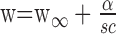5

Here, w_∞ is the asymptotic optimal filter width for high speed and contrast, and α is a constant. These parameters were selected to minimize the squared error between log₁₀(w) and the prediction from Equation 5, for pooled data from three preparations. The data and fit are shown superimposed in Figure 5D. The asymptotic optimal filter width w_∞ obtained from this fit was 15 msec.

Temporal resolution and interspike intervals

The optimal filter width can be used to obtain a meaningful measure of the number of spikes that typically convey the elementary motion signal. If the interspike interval (ISI) is always much larger than the filter width, optimal motion sensing preserves the distinction between sequential spikes, and motion information is effectively conveyed by individual spike times. Conversely, if the ISI is always much smaller than the filter width, optimal motion sensing integrates over many spikes, and motion information is effectively conveyed by variations in firing rate. The ratio of ISI to optimal filter width was accumulated across all of the spike trains from all conditions in three preparations; its distribution is shown in Figure 6. The modal ratio was ∼1, the median was 1.33, and 42% of values were <1. Note that this distribution includes ISIs during maintained firing before and after the moving bar crossed the receptive field; the ratios would be expected to be somewhat smaller for evoked spikes only. The similarity of optimal filter width and ISIs suggests that accurate motion sensing typically requires interpolating over one to a few spikes to compare the timing of responses in different cells. Note, however, that the ratio of ISI to filter width spans a wide range.

Figure 6.

Ratio of ISI to optimal filter width (τ) for direction discrimination accumulated across all spike trains from all conditions in three preparations. Not shown are 0.1% of values that lie outside the range of the plot.

Technical considerations

Estimates of temporal resolution could be artificially coarse if the delays used in computing motion signals (Fig. 2) differed from the true time differences in responses of different cells to the moving bar. This could result from error in estimated receptive field location (see Materials and Methods), receptive field microstructure not captured by a Gaussian model (Chichilnisky and Baylor, 1999b; Brown et al., 2000), or spatial and temporal sampling of the stimulus introduced by the display. To control for these possibilities, delays were obtained directly from moving bar data by identifying the peak in the cross-correlogram of response histograms averaged across all trials and smoothed with a 1 msec filter. The median optimal filter width across all conditions with delays obtained this way was 19 msec; the 10th and 19th percentiles were 9 and 50 msec, respectively. Asymptotic filter width was 13 msec. Thus, the two methods of estimating response delays yielded similar results.

The coarse temporal resolution observed was not attributable to artificially low evoked firing rates in the in vitro preparation. In the three preparations examined, peak firing rates measured in 25 msec bins for 96% contrast bars at intermediate speeds were 121 ± 18, 116 ± 24, and 93 ± 19 Hz, respectively (mean ± SD across cells). A previous in vivo study of macaque RGCs (Kremers et al., 1993) documented peak firing rate in 25 msec bins averaged across six magnocellular-projecting cells in response to stimuli temporally modulated at 1.22 Hz. As stimulus contrast approached 100%, peak firing rate increased to ∼60 Hz for sinusoidal modulation and 120 Hz for square-wave modulation. Because a moving bar has a sharp edge but enters the receptive field gradually, peak firing rates in response to a moving bar would be expected to fall in this range, as was observed.

In addition, randomly subsampling half of the spikes from each cell (10 iterations) on each trial of the moving stimulus yielded median optimal filter width of 28 msec across all conditions; 10th and 19th percentiles were 13 and 63 msec, respectively. Asymptotic filter width was 17 msec. Because evoked firing rates were within a factor of 2 of what would be expected in vivo (see above), this suggests that the optimal filter widths that would apply to parasol cells in vivo are similar to the values reported here.

The observed temporal resolution was not restricted to the specific functional form of the filter used. This was determined by estimating SNR as a function of the width (standard deviation) of a Gaussian filter applied to spike trains. The median optimal filter width obtained this way was 17 msec; 10th and 19th percentiles were 8 and 41 msec, respectively. Asymptotic filter width was 10 msec.

The observed temporal resolution was not dependent on the pairwise construction of the cross-correlation algorithm used to read out the direction of motion. This can be seen by noting that the algorithm is mathematically equivalent to a multicell computation in which the left and right motion signals are created by appropriately delaying responses from each cell, summing and squaring all of the responses pointwise, and integrating the result over time (see Materials and Methods).

Temporal resolution on the order of tens of milliseconds was also observed using the following alternative algorithm for motion sensing. If responses from different cells were identical up to an overall scaling of response amplitude, then the first principal component would explain all of the variance in the time course of response across cells. The fraction of the total variance explained by the first principal component therefore provides an index of the alignment of the responses of different cells. This was applied to motion sensing by temporally filtering responses of all cells in each trial, then computing the difference between the index of alignment obtained for responses delayed according to leftward and rightward motion. This value was used to discriminate direction of motion, and the SNR of its distribution across trials was examined as a function of filter width, as above. The median optimal filter width across all conditions was 28 msec; 10th and 19th percentiles were 16 and 59 msec, respectively. Asymptotic filter width was 18 msec.

Discussion

The present results indicate that direction of motion can be most accurately extracted from primate RGC spike trains by temporally filtering by 10-50 msec, effectively interpolating the gaps between spikes, before comparing the timing of responses in different cells. This defines the time scale for reading the population code, assuming readout based on linear filtering and cross-correlation. Despite the fact that direction sensing relies entirely on spike timing, the millisecond precision that is sometimes observed in RGC spike trains is of little consequence in this task. Indeed, the results suggest that motion-sensitive neurons in the visual cortex could filter their inputs coarsely in time at the synapse, rather than relying on the precise times of individual input spikes, to sense motion most reliably.

Time scales of neural signals

Numerous studies have examined whether the precise times of individual spikes, rather than slowly varying firing rates, are used to transmit information in the visual system and other areas of the brain (Abeles et al., 1993; Softky and Koch, 1993; Rieke et al., 1997; Shadlen and Newsome, 1998). This question is difficult to answer decisively, in part because of the lack of an unambiguous distinction between the two hypotheses. A useful approach is to first determine the time scale that is appropriate for reading out neural signals in the context of a behaviorally significant task in which the relevant neurons have been identified (de Ruyter van Steveninck and Bialek, 1988; Rieke et al., 1997). In the present work, this approach revealed an optimal time scale for decoding parasol RGC signals that subserve motion sensing. This time scale, in turn, defines how motion is encoded in spike trains. If motion were encoded in the precise times of individual spikes, an optimal filter width significantly smaller than the typical ISI would be expected, to avoid spurious motion signals caused by maintained firing. If motion signals were instead encoded by slow variations in firing rate, an optimal filter width significantly larger than the typical ISI would be required to obtain an accurate rate estimate (rate estimates cannot be obtained by pooling over many cells, because parasol cells and other RGC types form mosaics that tile the visual field without overlap) (Rodieck, 1998). In fact, the observed ratio of ISI to filter width varied widely, but the modal value was ∼1. This suggests an intermediate conclusion: on the time scale dictated by the statistics of the spike train and the demands of the task, one to a few spikes are typically available, similar to the situation in the fly visual system (Rieke et al., 1997). Note that a filter width on the order of the ISI has the advantage of providing an estimate of motion that is smooth in time.

Of course, aspects of visual performance outside the scope of this study may demand finer or coarser filtering than is optimal for direction sensing. A filter width of 1 msec on average yields a direction discrimination SNR that is only 53% as high as that obtained with a filter width of 10 msec (Fig. 4), but this reduction in SNR could be acceptable if retaining precise temporal information served other purposes. For example, a finer filter would narrow the speed tuning of motion detectors. Also, the precise times of spikes could be used by the brain for other visual tasks such as determining the time of stimulus onset.

Temporal resolution and spike timing precision

The temporal resolution observed in this study was approximately an order of magnitude coarser than the finest temporal precision of spiking observed in individual RGCs of salamander and rabbit (Berry et al., 1997; Berry and Meister, 1998) and macaque (V. J. Uzzell and E. J. Chichilnisky, unpublished observations) as well as LGN neurons (Reinagel and Reid, 2000; Liu et al., 2001). At least four factors contribute to this difference.

First, previous reports emphasized the maximum precision observed in spike trains that display both low and high precision. It seems unlikely that direction-selective neurons in the brain use only the most precise segments of input spike trains to compute motion and selectively exclude other informative spikes (but see Usrey et al., 1998), so in the present work, motion readout was performed using all spikes. The coarse resolution observed indicates that the benefits of using the coarse temporal information conveyed by most spikes overwhelms any advantage that might be obtained from precise temporal information conveyed by a minority of spikes. Thus, the temporal resolution of motion readout reflects the typical, rather than the extreme, precision of RGC spikes.

Second, RGC spike trains exhibit unreliability (spike count variability) that is typically factored out in estimates of spike timing precision. Unreliability in sparse spike trains demands coarser temporal filtering by postsynaptic neurons to obtain an accurate estimate of input activity. This is particularly important for computations such as motion sensing that involve comparing the activity of two or more inputs, because most or all of the inputs must be active to perform the comparison.

Third, previous studies examined responses to full-field stimuli, which may elicit precisely timed spikes by simultaneously activating many synapses, bringing membrane potential to threshold too rapidly to be significantly affected by voltage fluctuations. The tapering receptive field profile of RGCs could make the onset of responses to moving stimuli more gradual and more variable. Full-field stimuli may elicit maximal precision, but moving bars may be more representative of naturally occurring stimuli of behavioral importance.

Finally, heterogeneity in the receptive field profiles of different cells (Chichilnisky and Baylor, 1999b; Brown et al., 2000) would result in different responses to moving stimuli, even in a collection of cells with homogeneous response kinetics (Chichilnisky and Kalmar, 2002; Reinagel and Reid, 2002). This would result in coarser temporal resolution, because motion sensing involves comparing the timing of different inputs.

Stimulus dependence

Temporal resolution declined with speed and contrast but was 10-50 msec for a wide range of conditions and approached a limit of ∼10 msec at high speeds and contrasts. It is unsurprising that temporal resolution should be coarse for low-contrast stimuli, because the resulting visual signals are noisy, and thus discrimination requires more temporal integration. However, the asymptotic behavior at high contrasts suggests that resolution is limited even for strong visual signals.

At speeds lower than a few degrees per second, temporal resolution approached values in excess of 50 msec. However, this is probably not functionally significant given that the preferred speeds of neurons in area MT fall mostly in the range 8-64 deg · sec^-1 and always in the range 2-512 deg · sec^-1 (Maunsell and Van Essen, 1983). At the other extreme, the asymptotic resolution at high speeds suggests that the statistics of RGC spiking impose a resolution limit. However, at the highest speed tested, spatial and temporal discretization imposed by the display was significant: the bar moved one bar width per frame (see Materials and Methods). Discretization could cause the delays between responses of different cells to deviate from expectations based on receptive field position and speed, thus artificially coarsening the estimated temporal resolution. However, allowing for arbitrary delays between cells had little effect on resolution. Thus, there appears to be a fundamental limit of ∼10 msec to the temporal resolution of motion signals, but additional investigation of responses to high-speed stimuli is merited.

Models of motion readout

Temporal resolution was analyzed by reading out retinal motion signals using low-pass filtering followed by cross-correlation as a computational tool. Motion sensing in the visual cortex is undoubtedly different in detail, but perhaps not in essential structure. Filtering and cross-correlation are the core elements in computational models of motion sensing in the brain (Reichardt, 1961; Adelson and Bergen, 1985; Watson and Ahumada, 1985; Simoncelli and Heeger, 1998), including models that differ in implementation. For example, the hierarchy of computations that creates cortical direction selectivity more closely resembles an opponent motion energy sensor than a Reichardt sensor (Emerson et al., 1992), but the input-output properties of these sensors can be identical, because they both rely on pairwise multiplication, or summing and squaring, of input signals filtered differently in time and space (Adelson and Bergen, 1985). The approach used here can also be described both ways (see Materials and Methods).

The principal difference between a motion energy sensor and the readout approach adopted here is that the latter is directly applicable to spike trains. Motion energy computations begin with noiseless, linear filtering of the visual scene. This is at best a crude approximation of retinal processing: responses of primate parasol RGCs are nonlinear (Benardete and Kaplan, 1999; Chichilnisky and Kalmar, 2002), sampled in space (finite number of cells) and time (spikes), noisy (Troy and Lee, 1994), and correlated (Mastronarde, 1983; Chichilnisky and Baylor, 1999a). Even if simplifying approximations were adopted, assembling the detailed spatiotemporal filters of a fully elaborated motion energy sensor using a discrete, incomplete set of RGC inputs is problematic. These issues arise, because motion energy models are applicable to image sequences in which input data are continuous, and noiseless and arbitrary filtering is possible. In contrast, the problem approached here is how to sense motion using real retinal spike trains.

The coarse temporal resolution observed was not restricted to motion readout based on pairwise cross-correlation: an approach that used the responses of all of the cells simultaneously was shown to be formally identical to the pairwise approach (see Materials and Methods). Also, motion readout using principal-components analysis instead of cross-correlation exhibited similar temporal resolution. However, the main readout approach examined—linear filtering followed by cross-correlation—is not guaranteed to be optimal or biologically accurate, and it is possible that other approaches would exhibit significantly different temporal resolution. The results reported here apply to a restricted but important class of motion sensing models.

Motion detectors were assumed to be tuned to the correct stimulus speed for simplicity. Neurons in area MT, which has an important role in motion sensing (Albright, 1984; Newsome et al., 1985; Salzman et al., 1990), are tuned for a range of speeds (Maunsell and Van Essen, 1983). If behavioral direction discrimination relies on a pool of cortical neurons with a range of speed tunings, the effective noise in the pool could exceed that of a single, correctly tuned motion detector. This could limit behavioral direction discrimination but probably would not change the temporal resolution of readout.

Implications for motion sensing in visual cortex

The timing of spikes in MT neurons elicited by moving stimuli can be reproducible to within a few milliseconds (Bair and Koch, 1996; Buracas et al., 1998). However, this precise time-locking to the stimulus does not reveal the time scale appropriate for comparing the timing of input spikes to sense motion. Indeed, high convergence may make it difficult for cortical neurons to exploit the precise timing of individual inputs (Shadlen and Newsome, 1998). Cortical neurons could fire spikes precisely time-locked to the stimulus by thresholding pooled inputs that are filtered coarsely in time at the synapse to sense motion reliably.

References

- Abeles M, Bergman H, Margalit E, Vaadia E ( 1993) Spatiotemporal firing patterns in the frontal cortex of behaving monkeys. J Neurophysiol 70: 1629-1638. [DOI] [PubMed] [Google Scholar]
- Adelson EH, Bergen JR ( 1985) Spatiotemporal energy models for the perception of motion. J Opt Soc Am A 2: 284-299. [DOI] [PubMed] [Google Scholar]
- Albright TD ( 1984) Direction and orientation selectivity of neurons in visual area MT of the macaque. J Neurophysiol 52: 1106-1130. [DOI] [PubMed] [Google Scholar]
- Bair W, Koch C ( 1996) Temporal precision of spike trains in extrastriate cortex of the behaving macaque monkey. Neural Comput 8: 1185-1202. [DOI] [PubMed] [Google Scholar]
- Benardete EA, Kaplan E ( 1999) The dynamics of primate M retinal ganglion cells. Vis Neurosci 16: 355-368. [DOI] [PubMed] [Google Scholar]
- Berry MJ, Meister M ( 1998) Refractoriness and neural precision. J Neurosci 18: 2200-2211. [DOI] [PMC free article] [PubMed] [Google Scholar]
- Berry MJ, Warland DK, Meister M ( 1997) The structure and precision of retinal spike trains. Proc Natl Acad Sci USA 94: 5411-5416. [DOI] [PMC free article] [PubMed] [Google Scholar]
- Bialek W, Rieke F, Steveninck RR, Warland D ( 1991) Reading a neural code. Science 252: 1854-1857. [DOI] [PubMed] [Google Scholar]
- Brown SP, He S, Masland RH ( 2000) Receptive field microstructure and dendritic geometry of retinal ganglion cells. Neuron 27: 371-383. [DOI] [PubMed] [Google Scholar]
- Buracas GT, Zador AM, DeWeese MR, Albright TD ( 1998) Efficient discrimination of temporal patterns by motion-sensitive neurons in primate visual cortex. Neuron 20: 959-969. [DOI] [PubMed] [Google Scholar]
- Chichilnisky EJ ( 2001) A simple white noise analysis of neuronal light responses. Network 12: 199-213. [PubMed] [Google Scholar]
- Chichilnisky EJ, Baylor DA ( 1999a) Synchronized firing by ganglion cells in monkey retina. Soc Neurosci Abstr 25: 1042. [Google Scholar]
- Chichilnisky EJ, Baylor DA ( 1999b) Receptive-field microstructure of blue-yellow ganglion cells in primate retina. Nat Neurosci 2: 889-893. [DOI] [PubMed] [Google Scholar]
- Chichilnisky EJ, Kalmar RS ( 2002) Functional asymmetries in ON and OFF ganglion cells of primate retina. J Neurosci 22: 2737-2747. [DOI] [PMC free article] [PubMed] [Google Scholar]
- Dacey DM, Petersen MR ( 1992) Dendritic field size and morphology of midget and parasol ganglion cells of the human retina. Proc Natl Acad Sci USA 89: 9666-9670. [DOI] [PMC free article] [PubMed] [Google Scholar]
- de Ruyter van Steveninck RR, Bialek W ( 1988) Real-time performance of a movement-sensitive neuron in the blowfly visual system: coding and information transfer in short spike sequences. Proc R Soc Lond B Biol Sci 234: 379-414. [Google Scholar]
- de Ruyter van Steveninck RR, Lewen GD, Strong SP, Koberle R, Bialek W ( 1997) Reproducibility and variability in neural spike trains. Science 275: 1805-1808. [DOI] [PubMed] [Google Scholar]
- Emerson RC, Bergen JR, Adelson EH ( 1992) Directionally selective complex cells and the computation of motion energy in cat visual cortex. Vision Res 32: 203-218. [DOI] [PubMed] [Google Scholar]
- Kraft TW ( 1988) Photocurrents of cone photoreceptors of the golden-mantled ground squirrel. J Physiol (Lond) 404: 199-213. [DOI] [PMC free article] [PubMed] [Google Scholar]
- Kremers J, Lee BB, Pokorny J, Smith VC ( 1993) Responses of macaque ganglion cells and human observers to compound periodic waveforms. Vision Res 33: 1997-2011. [DOI] [PubMed] [Google Scholar]
- Litke AM ( 1999) The retinal readout system: a status report. Nucl Instrum Methods Phys Res A 435: 242-249. [Google Scholar]
- Liu RC, Tzonev S, Rebrik S, Miller KD ( 2001) Variability and information in a neural code of the cat lateral geniculate nucleus. J Neurophysiol 86: 2789-2806. [DOI] [PubMed] [Google Scholar]
- Mastronarde DN ( 1983) Interactions between ganglion cells in cat retina. J Neurophysiol 49: 350-365. [DOI] [PubMed] [Google Scholar]
- Mastronarde DN, Humphrey AL, Saul AB ( 1991) Lagged Y cells in the cat lateral geniculate nucleus. Vis Neurosci 7: 191-200. [DOI] [PubMed] [Google Scholar]
- Maunsell JH, Van Essen DC ( 1983) Functional properties of neurons in middle temporal visual area of the macaque monkey. I. Selectivity for stimulus direction, speed, and orientation. J Neurophysiol 49: 1127-1147. [DOI] [PubMed] [Google Scholar]
- Meister M, Pine J, Baylor DA ( 1994) Multi-neuronal signals from the retina: acquisition and analysis. J Neurosci Methods 51: 95-106. [DOI] [PubMed] [Google Scholar]
- Meister M, Lagnado L, Baylor DA ( 1995) Concerted signaling by retinal ganglion cells. Science 270: 1207-1210. [DOI] [PubMed] [Google Scholar]
- Newsome WT, Wurtz RH, Dursteler MR, Mikami A ( 1985) Deficits in visual motion processing following ibotenic acid lesions of the middle temporal visual area of the macaque monkey. J Neurosci 5: 825-840. [DOI] [PMC free article] [PubMed] [Google Scholar]
- Perry VH, Cowey A ( 1985) The ganglion cell and cone distributions in the monkey's retina: implications for central magnification factors. Vision Res 25: 1795-1810. [DOI] [PubMed] [Google Scholar]
- Polyak SL ( 1941) The retina. Chicago: University of Chicago.
- Reich DS, Victor JD, Knight BW, Ozaki T, Kaplan E ( 1997) Response variability and timing precision of neuronal spike trains in vivo. J Neurophysiol 77: 2836-2841. [DOI] [PubMed] [Google Scholar]
- Reichardt W ( 1961) Autocorrelation, a principle for the evaluation of sensory information by the central nervous system. In: Sensory communication (Rosenblith WA, ed), pp 303-317. Cambridge, MA: MIT.
- Reinagel P, Reid RC ( 2000) Temporal coding of visual information in the thalamus. J Neurosci 20: 5392-5400. [DOI] [PMC free article] [PubMed] [Google Scholar]
- Reinagel P, Reid RC ( 2002) Precise firing events are conserved across neurons. J Neurosci 22: 6837-6841. [DOI] [PMC free article] [PubMed] [Google Scholar]
- Rieke FM, Warland D, Steveninck RR, Bialek W ( 1997) Spikes: exploring the neural code, Ed 1. Cambridge, MA: MIT.
- Rodieck RW ( 1998) The first steps in seeing, Ed 1. Sunderland, MA: Sinauer.
- Sakai HM, Naka K, Korenberg MJ ( 1988) White-noise analysis in visual neuroscience. Vis Neurosci 1: 287-296. [DOI] [PubMed] [Google Scholar]
- Salzman CD, Britten KH, Newsome WT ( 1990) Cortical microstimulation influences perceptual judgements of motion direction. Nature 346: 174-177. [DOI] [PubMed] [Google Scholar]
- Schnapf JL, Nunn BJ, Meister M, Baylor DA ( 1990) Visual transduction in cones of the monkey Macaca fascicularis J Physiol (Lond) 427: 681-713. [DOI] [PMC free article] [PubMed] [Google Scholar]
- Shadlen MN, Newsome WT ( 1998) The variable discharge of cortical neurons: implications for connectivity, computation, and information coding. J Neurosci 18: 3870-3896. [DOI] [PMC free article] [PubMed] [Google Scholar]
- Simoncelli EP, Heeger DJ ( 1998) A model of neuronal responses in visual area MT. Vision Res 38: 743-761. [DOI] [PubMed] [Google Scholar]
- Softky WR, Koch C ( 1993) The highly irregular firing of cortical cells is inconsistent with temporal integration of random EPSPs. J Neurosci 13: 334-350. [DOI] [PMC free article] [PubMed] [Google Scholar]
- Troy JB, Lee BB ( 1994) Steady discharges of macaque retinal ganglion cells. Vis Neurosci 11: 111-118. [DOI] [PubMed] [Google Scholar]
- Usrey WM, Reppas JB, Reid RC ( 1998) Paired-spike interactions and synaptic efficacy of retinal inputs to the thalamus. Nature 395: 384-387. [DOI] [PubMed] [Google Scholar]
- Van Essen DC ( 1985) Functional organization of primate visual cortex. In: Cerebral cortex, Vol III (Peters A, Jones EG, eds), pp 259-327. New York: Plenum. [Google Scholar]
- Watanabe M, Rodieck RW ( 1989) Parasol and midget ganglion cells of the primate retina. J Comp Neurol 289: 434-454. [DOI] [PubMed] [Google Scholar]
- Watson AB, Ahumada AJ ( 1985) Model of human visual-motion sensing. J Opt Soc Am A 2: 322-341. [DOI] [PubMed] [Google Scholar]