Macaque Middle Temporal Neurons Signal Depth in the Absence of Motion

Abstract

The middle temporal (MT) visual area is widely accepted to play important roles in motion processing. It is unclear, however, whether MT contributes to visual perception during the viewing of static scenes, when there is little retinal image motion during the interval between saccades. Some previous studies suggest that MT neurons give little or no response to stationary stimuli that are flashed onto the receptive field, but no previous study has directly examined the fidelity with which MT neurons code visual information in moving versus stationary stimuli. In this study, we compare the ability of MT neurons to signal binocular disparity in moving versus stationary random-dot stereograms. Although responses to moving stimuli are typically stronger, many MT neurons give robust responses to stationary stereograms, and some MT neurons actually prefer stationary patterns to those moving at any tested speed. These responses to stationary stimuli are not caused by monitor refresh or microsaccades. Disparity tuning curves for moving and stationary stimuli are nearly identical in shape for most neurons. Although the disparity discriminability of MT neurons is generally higher for moving stereograms when responses are averaged over the entire 1.5 sec trial epoch, discriminability is comparable for moving and stationary stimuli during the first 200-300 msec of the response. Thus, in a normal time interval between saccades, MT neurons signal the binocular disparity of stationary stimuli with high fidelity. These findings show that MT can be a reliable source of visual information during the viewing of static scenes.

Introduction

In most modern schemes for the organization of primate visual pathways (Maunsell and Newsome, 1987; Felleman and Van Essen, 1991; Van Essen and Gallant, 1994), the middle temporal (MT) visual area occupies an important position as a central gateway for information flow from early visual areas (e.g., V1, V2, V3) to the parietal cortex. Area MT is known to play important roles in the processing of visual motion information for perception (for review, see Albright, 1993; Parker and Newsome, 1998) and for guiding eye movements (Newsome et al., 1985; Komatsu and Wurtz, 1989; Schiller and Lee, 1994; Groh et al., 1997; Lisberger and Movshon, 1999). Consistent with these roles, virtually all MT neurons exhibit strong selectivity for the direction and speed of moving stimuli (Zeki, 1974; Maunsell and Van Essen, 1983a; Albright, 1984; Rodman and Albright, 1987; Snowden et al., 1992; Lagae et al., 1993; DeAngelis and Uka, 2003). Notably, most previous studies show that MT neurons give little response to bar stimuli that move very slowly (Maunsell and Van Essen, 1983a; Mikami et al., 1986; Cheng et al., 1994; but see Lagae et al., 1993, and Discussion). Moreover, MT neurons generally respond poorly and transiently, if at all, to stationary bars that are flashed onto the receptive field (Maunsell and Van Essen, 1983a; Albright, 1984; Marcar et al., 1995).

If MT neurons are typically inactive when there is no motion in their receptive fields, MT may provide little useful information when a subject fixates from point to point within a stationary scene (ignoring, for now, the brief pulses of retinal image motion that accompany saccades) (see Discussion). How, then, does visual information flow from early visual areas to the parietal lobe? One possibility is that other areas provide the main parietal input in these instances, and the anatomy certainly supports this possibility (Lewis and Van Essen, 2000). However, it seems premature to exclude the possibility that MT still serves as a major conduit for visual information in the absence of retinal image motion. To our knowledge, no previous study has directly compared the fidelity with which MT neurons signal visual information in stationary versus moving stimuli. Perhaps this is because most previous studies of MT have focused on the coding of motion itself.

We therefore measured the binocular disparity tuning of MT neurons in response to stereograms containing either stationary dots or dots moving at the preferred speed of each neuron. Coding of disparity seems an obvious choice for this analysis, because >90% of MT neurons are disparity selective (Maunsell and Van Essen, 1983b; DeAngelis and Uka, 2003), and because MT has been shown to contribute to monkeys' judgments of depth (DeAngelis et al., 1998). We report that many MT neurons give robust, sustained responses to stationary random-dot stereograms that are flashed onto the receptive field, and we show that these responses are not attributable to the occurrence of microsaccades during fixation. Disparity tuning curves for stationary stimuli are nearly identical to those for moving stimuli, although responses to stationary dots are usually weaker. Importantly, the disparity discriminability of MT neurons is similar for moving and stationary stimuli during the first few hundred milliseconds of the response (a typical interval between saccades in normal vision). Our findings thus show that MT carries robust visual information in the absence of motion.

Materials and Methods

Experiments were performed on two male rhesus monkeys (Macaca mulatta) weighing 5-6 kg. All of the experimental procedures were approved by the Institutional Animal Care and Use Committee at Washington University and conformed with National Institutes of Health guidelines.

Surgical preparation. Animals were prepared for daily training and recording sessions using standard surgical procedures (Britten et al., 1992; DeAngelis and Newsome, 1999). Briefly, a head post (for head restraint) and recording chamber were implanted and affixed to the skull using the combination of titanium screws and cranioplastic cement (Plastics One, Roanoke, VA). The recording chamber was centered over the occipital cortex at a location roughly 17 mm lateral and 14 mm dorsal to the occipital ridge. The chamber was affixed in a parasagittal plane and was oriented 25° above horizontal. An eye coil was implanted under the conjunctiva in each eye, allowing us to monitor both conjugate eye position as well as vergence angle. To reduce coil slippage in the eye, each eye coil was sutured to the sclera using either a permanent or long-lasting dissolvable suture. As discussed previously in detail (DeAngelis and Uka, 2003), monkeys' vergence posture was under tight control, and vergence errors had a negligible impact on our disparity-tuning measurements.

Visual stimuli and task. Visual stimuli consisted of random-dot stereograms (RDSs) that were generated by an OpenGL accelerator board (Oxygen GVX1; 3Dlabs, Milpitas, CA) and presented on a 22 inch color display (GDM-F500; Sony, Tokyo, Japan) subtending 40 × 30° at a viewing distance of 57 cm (Fig. 1). Dot density was 64 dots · deg ^-2 · sec ^-1, and each dot subtended ∼0.1°. The starting position of each dot within the receptive field was newly randomized for each trial. Precise disparities and smooth motion were achieved by plotting dots with subpixel resolution using the hardware antialiasing capabilities of the OpenGL accelerator. Left and right half-images were presented alternately at a refresh rate of 100 Hz, and stereoscopic presentation was achieved using ferro-electric liquid crystal shutters (DisplayTech, Longmont, CO) that were synchronized to the video refresh. To minimize ghosting (stereo crosstalk was <3%), the RDS consisted of red dots presented on a black background. Additional details regarding stimulus generation have been described previously (DeAngelis and Uka, 2003). Note that the 100 Hz refresh rate and the frame-alternation stereoscopic technique limited the speeds of motion that we could present. A maximal speed of 32 deg/sec was chosen, because the motion was still quite smooth at this speed.

Figure 1.

Illustration of the visual stimulus used in these experiments. The small black square is the fixation point, and the dashed circle (not present in the actual display) denotes the receptive field of a typical MT neuron. Dots outside the receptive field were stationary and always presented with zero binocular disparity. Dots within the receptive field could move at a variety of different speeds and were presented at different horizontal disparities (indicated here as pairs of horizontally separated dots). In the actual displays, stimuli consisted of red dots on a black background and were viewed stereoscopically using ferroelectric shutter glasses. Bottom traces show the onset and offset timing of the fixation point, dots, and reward.

Monkeys viewed the random-dot stimuli while maintaining fixation on a small yellow spot (0.15°). The fixation window was typically 1.5° full width. Stimuli were presented for a period of 1.5 sec, and monkeys received a liquid reward for maintaining fixation throughout this period (Fig. 1). When the monkey's conjugate eye position left the fixation window during the trial, the visual stimulus was terminated, data were discarded, and the monkey was not rewarded. Both monkeys were initially trained to maintain their vergence angle within ±0.25° of the plane of fixation. A background of stationary dots presented at zero disparity helped to anchor vergence, and vergence posture was measured during all of the recording experiments.

Recording procedures and data acquisition. Tungsten microelectrodes (FHC, Bowdoinham, ME) were introduced into the cortex through a transdural guide tube and typically passed through extrastriate visual areas in the anterior bank of the lunate sulcus before entering area MT. MT was recognized on the basis of extensive experience interpreting the patterns of gray- and white-matter transitions along electrode penetrations, the response properties of single units (SUs) and multiunit (MU) clusters (direction, speed, and disparity tuning), the relationship between receptive-field size and eccentricity, and the subsequent entry into gray matter with response properties typical of area MST. All of the data included in this study were derived from recordings that were confidently assigned to area MT.

Behavioral control and data acquisition were accomplished using a commercially available software package (Tempo; Reflective Computing, St. Louis, MO). Raw neural signals were amplified, bandpass filtered (500-5000 Hz), and discriminated using conventional electronic equipment (Bak Electronics, Mt. Airy, MD). Only well isolated action potentials were counted as SU responses. In contrast, MU activity was defined as any deflection of the analog signal that exceeded a threshold level set using the window discriminator. Because the absolute frequency of MU activity depends arbitrarily on the threshold level used, we adjusted the threshold level to obtain a roughly consistent frequency of spontaneous activity (∼100 events/sec) at each recording site (DeAngelis and Newsome, 1999).

Times of occurrence of SU and MU events, along with behavioral event markers, were stored to disk with 1 msec resolution. Horizontal and vertical eye position signals from each eye were sampled at 1 kHz and stored to disk at a rate of 250 Hz.

Experimental protocol and data analysis. We first thoroughly explored the receptive field and tuning properties of each isolated MT neuron using a receptive field mapping program. Receptive field location and size were carefully determined, and the preferred direction, speed, and disparity were estimated.

Subsequently, we quantitatively measured the direction, speed, and horizontal disparity selectivity of each neuron (or multiunit cluster) by presenting random-dot stimuli in blocks of randomly interleaved trials. First, a direction tuning curve was obtained by presenting eight directions of motion, 45° apart. Responses of the neuron were computed for each direction of motion (θ), and these data were fit with a Gaussian of the form:

1

where R₀ is the baseline level of the curve, A is the amplitude of the Gaussian, θ₀ is the location of the center of the Gausian (i.e., the preferred direction of the neuron), and σ is the SD. The best fit of this function was achieved by minimizing the sum squared error between the responses of the neuron and the values of the function (using the constrained minimization tool, fmincon, in Matlab). To homogenize the variance of the neural responses across different stimulus conditions, we minimized the difference between the square root of the neural responses and the square root of the Gaussian (Prince et al., 2002). This approach was used for all of the curve fits in this study. Additional details regarding tuning measurements and curve fits have been described previously (DeAngelis and Uka, 2003).

Next, we measured a speed tuning curve for each neuron after adjusting the stimulus to the preferred direction of the neuron, determined as above. Typically, we presented speeds of 0, 0.5, 1, 2, 4, 8, 16, and 32 deg/sec, and we averaged responses across four to five stimulus repetitions. Each speed tuning curve was fit with a Gamma distribution of the form:

2

where s is the stimulus speed, and R₀, A, α, τ, and n are free parameters. The Gamma distribution varies in shape from an exponential to a Gaussian depending on the value of the exponent n. The denominator term normalizes the curve to have an amplitude specified by A. We found that this function provided excellent fits to the vast majority of our speed tuning curves (mean R², 0.97; range, 0.52-1; n = 395), as can be seen from the examples shown in Figure 2 (left). The preferred speed of each neuron was taken as the speed at which the fitted curve reached its maximum value.

Figure 2.

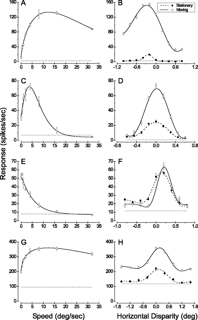
Speed and disparity tuning curves for four exemplary MT units (one unit per row). A, C, E, G, The speed tuning curve for each unit is shown. The mean response ± SE is shown for each tested speed (open circles with error bars), and the dotted horizontal line gives the spontaneous discharge rate when there was no stimulus in the receptive field. Solid curves show the Gamma distribution (Eq. 2) that best fit each set of data. B, D, F, H, The disparity tuning curves measured using both moving (open circles) and stationary (filled circles) random-dot stereograms are shown. Solid curves show the Gabor functions (Eq. 3) that were fit independently to each tuning curve. A, B, Data from a single unit that preferred fast speeds and gave little response to stationary dots. Receptive field size, 7.5°; eccentricity, 8.7°; speed of moving dots, 10 deg/sec; SMRR, 0.08. C, D, Data from a modal single unit that exhibited moderate responses to stationary dots. Receptive field size, 8.5°; eccentricity, 9.2°; speed of moving dots, 4 deg/sec; SMRR, 0.42. E, F, One of a handful of striking MT units that responded preferentially to stationary stimuli. Receptive field size, 7.5°; eccentricity, 8.3°; speed of moving dots, 0.5 deg/sec; SMRR, 0.98. G, H, Data from a modal multiunit recording. Note the clear shift in baseline firing level between the two disparity tuning curves. Receptive field size, 9.1°; eccentricity, 11.4°; speed of moving dots, 10 deg/sec; SMRR, 0.39.

Finally, we measured a disparity tuning curve using both stationary dots (0 deg/sec) and dots moving at the preferred direction and speed of the neuron. For a handful of cases in which zero speed was optimal, moving dots were presented at a very slow speed (usually 0.5 or 1 deg/sec). In most cases, disparities were tested from -1.6 to 1.6° in steps of 0.4°; however, these parameters were adjusted as necessary on the basis of our initial qualitative assessment of the breadth of disparity tuning. Each disparity tuning curve was fit with a Gabor function having the following form:

3

where d is the stimulus disparity, R₀ is the baseline response level, A is the amplitude, d₀ is the center of the Gaussian envelope, σ is the SD of the Gaussian, f is the frequency of the sinusoid, and φ is the phase of the sinusoid (relative to the center of the Gaussian). Because the disparity frequency (f) is often poorly constrained by the data at the low-frequency end, this parameter was only allowed to vary within ±10% of the disparity frequency determined from a Fourier transform of the raw tuning curve (Prince et al., 2002; DeAngelis and Uka, 2003). Gabor functions generally provided excellent fits to our disparity tuning curves (mean R², 0.91 and 0.95, for stationary and moving stimuli, respectively; n = 74 for each), as can be seen from the examples in Figures 2 and 4, A and C, as well as from the R² values given in Figure 4 E (horizontal axis).

Figure 4.

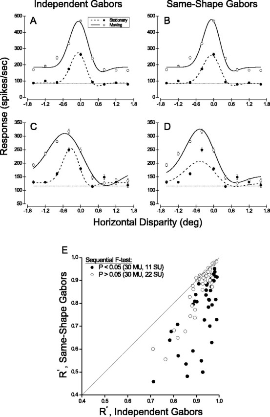
A Gabor-fitting analysis for testing whether the shapes of disparity tuning curves are the same for moving and stationary stimuli. A, Disparity tuning curves for moving and stationary dots (open and filled circles, respectively) are fit with independent Gabor functions. B, Data for the same multiunit are fit with a pair of Gabor functions that are constrained to have identical shapes, but independent amplitudes and baseline firing rates. C, Independent fits of Gabor functions to disparity tuning curves for another MT multiunit recording. D, The data set of C is fit with a pair of Gabor functions having identical shapes. In this case, the constrained fit is significantly worse than the independent fits (sequential F test; p << 0.001). E, Summary of independent and shape-constrained Gabor fits for 93 of 118 MT units that had significant disparity tuning for both moving and stationary stimuli. R² values for the shape-constrained fits are plotted against R² values for the independent fits. Units for which the same-shape fits were significantly worse than the independent fits are denoted by filled symbols (sequential F test; p < 0.05).

From each disparity tuning curve, we extracted three key measures: preferred disparity, disparity tuning index (DTI), and disparity discrimination index (DDI). The preferred disparity was defined as the disparity at which the Gabor fit reached its peak. For a handful of tuned-inhibitory neurons, for which the tuning curve consisted primarily of a trough, the disparity of the trough was taken instead. The amount of response modulation in each disparity tuning curve was assessed using the DTI:

4

where R_max and R_min are the maximum and minimum responses, respectively. To keep this index restricted to the range from 0 to 1, spontaneous activity was not subtracted from R_max or R_min. Finally, to characterize the the ability of the neuron to discriminate between their preferred and antipreferred disparities, we used the DDI (Prince et al., 2002):

5

where SSE is the sum squared error around the mean responses, N is the number of observations (trials), and M is the number of disparities tested. This index differs importantly from the DTI in that it takes into account the variability of the neural responses. This is quite useful given that stationary and moving stimuli often elicited different maximal responses and therefore also had different variances.

Statistical analyses. Our data set consisted of a mixture of multiunit and single-unit recordings from two different monkeys. Because differences in the average values of parameters between monkeys or between single and multiunit data could produce misleading correlation coefficients, all of the correlation analyses were done using a within-cells regression in the context of an analysis of covariance (ANCOVA). Monkey identity and recording type (single-unit or multiunit) were independent factors. Thus, all of the correlation coefficients and p values reported here are corrected for variations in these factors.

To evaluate different models that were fit to the disparity tuning curves of MT neurons (see Fig. 4), we used a sequential F test (Draper and Smith, 1966) to compare the errors associated with two different models, while allowing for differences in their degrees of freedom. Strictly speaking, this test should be used only to evaluate models that are linear in their parameters. To address this issue, we fit curves to many sets of artificial data that were generated by sampling spike rates from a Poisson distribution. These Monte Carlo simulations showed that the distribution of our F statistic was statistically indistinguishable from that of a real F distribution with the appropriate degrees of freedom (χ² test; p > 0.4). Thus, in this instance, it is appropriate to use the sequential F test to evaluate our models.

Analysis of eye movements. To test whether responses to stationary stimuli might have been driven by small eye movements within the fixation window, we constructed saccade-triggered averages of the neuronal responses (see Fig. 12). Fixational microsaccades were defined as changes in eye position that exceeded a velocity threshold of 8 deg/sec (Bair and O'Keefe, 1998). We constructed the saccade-triggered average by clipping out and averaging the neuronal responses around each fixational saccade (from 50 msec presaccade to 300 msec postsaccade). The saccade-triggered average was then smoothed with a Gaussian kernel having a SD of 6 msec.

Figure 12.

Examples of saccade-triggered averages. A, Speed tuning curve for an MT multiunit that preferred moderately fast speeds. Format is as in Figure 2A. B, Saccade-triggered average for the same MT multiunit. The thin curve is the raw saccade-triggered spike average. The thick curve is the same data after smoothing with a Gaussian kernel with SD of 6 msec. Note the clear peak after microsaccades. C, Speed tuning curve for an MT single unit that responded optimally to stationary dots and gave no response to movement faster than 2 deg/sec. D, Saccade-triggered average for this single unit shows a clear suppression of response after microsaccades.

Results

Our main data set consists of 76 multiunit clusters and 42 single units, recorded from two animals, for which we measured disparity tuning in response to both moving and stationary stimuli. In addition, speed tuning curves from an additional 277 single units were analyzed to quantify the relative strength of responses to stationary and moving stimuli.

Figure 2 shows four examples of data sets that illustrate the range of our observations. The single unit of Figure 2, A and B,is typical of many neurons that prefer higher speeds: it gives little response to stationary stimuli, but even this weak response exhibits clear disparity tuning. The examples of Figure 2, C and D, and G and H, are modal, exhibiting moderate responses to stationary stimuli and having nearly identical disparity tuning for moving and stationary patterns. The single unit of Figure 2, E and F,isone of several remarkable data sets in which stationary stimuli elicited a stronger response than stimuli moving at any speed within the range tested. Disparity tuning curves for stationary and moving random-dot stimuli were also very similar for this neuron. It is worth noting that a few multiunit recordings also exhibited low-pass speed tuning like that of Figure 2E; this suggests that neurons preferring stationary stimuli are clustered in MT, consistent with previous reports of speed clustering in MT (Maunsell and Van Essen, 1983a; DeAngelis and Newsome, 1999; Liu and Newsome, 2003).

Relative strength of responses to stationary and moving stimuli

To summarize the relative responses of MT neurons to stationary and moving stimuli, we divided the response (mean firing rate across the 1.5 sec stimulus period - spontaneous activity) obtained at zero speed by the response obtained at the preferred speed for each data set. These stationary:moving response ratios (SMRRs) are plotted as a function of preferred speed in Figure 3A for the single-unit and multiunit recordings that were studied in detail (large filled and unfilled circles, respectively). In addition, data are shown from a large sample of single units (n = 277; small filled squares) for which speed tuning curves were measured during the course of other studies. There is a pronounced negative correlation (ANCOVA within-cells regression, r = -0.51; p << 0.001) between the SMRR and preferred speed in Figure 3A, such that neurons preferring slower speeds exhibit stronger responses to stationary stimuli. Among all of the single units, 34% (107 of 319) exhibit responses to stationary stimuli that are at least one-third as large as those elicited by moving stimuli. Thus, robust responses to stationary stimuli are encountered fairly frequently in MT. Note also that the value of the SMRR depends strongly on the length of the analysis window, because responses to stationary stimuli typically have a strong transient component (as discussed later) (see Fig. 8). SMRR values would increase substantially if spikes were counted over only the first few hundred milliseconds of the response.

Figure 3.

Summary of speed tuning data for a large sample of MT units. In each scatter plot, large filled and open circles represent single units (n = 42) and multiunits (n = 76), respectively, for which we measured disparity tuning, using both moving and stationary stimuli. Small, black squares represent single units for which speed tuning curves were obtained as part of other studies (n = 277). A, SMRR (see Results) is plotted against the preferred speed for each MT unit. Note that there is an inverse relationship, such that neurons preferring slow speeds give strong responses to stationary stimuli. B, SMRR is plotted as a function of the receptive field eccentricity of each MT unit. C, Preferred speed is plotted against eccentricity.

Figure 8.

Population responses of MT units to moving (dashed curves) and stationary (solid curves) stimuli. For each unit, spontaneous activity was subtracted, and PSTHs were normalized by the peak response to moving dots. PSTHs were then averaged across neurons. Thick curves represent the subpopulation of MT units with SMRR > 0.33. Thin curves are the average of units with SMRR < 0.33. A, Population responses for all of the multiunit recordings (n = 76). B, Population responses for all of the single units (n = 42).

Figure 3B shows that neurons with strong responses to stationary dots are distributed quite uniformly over the range of eccentricities (∼2-15°) at which we recorded (r = 0.10; p = 0.042). This might appear to be surprising if one expects preferred speeds to increase with eccentricity. However, we found no such correlation, as shown in Figure 3C (r = 0.06; p = 0.22). This result is consistent with those of two previous studies based on smaller sample sizes (Maunsell and Van Essen, 1983a; Lagae et al., 1993). It is also worth noting that relatively few neurons in Figure 3C have preferred speeds of >25 deg/sec. This appears to conflict with some previous studies of speed tuning in MT that have used bar stimuli in anesthetized animals; this issue will be addressed in Discussion.

Comparison of disparity tuning for stationary and moving stimuli

From the examples of Figure 2, it appears that disparity tuning curves for stationary and moving stimuli generally have the same shape, differing only in the amplitude and/or baseline level of response. To test this notion quantitatively, we used a model-based approach to analyze data from the subset of units (60 of 76 multiunit clusters; 33 of 42 single units) with significant disparity tuning (ANOVA; p < 0.05) for both moving and stationary stimuli. First, we fit the two disparity tuning curves for each neuron with independent Gabor functions, as shown in Figures 2 and 4, A and C. These independent Gabor fits accounted for a high percentage of the variance in neural responses to different disparities (Fig. 4E, horizontal axis).

Next, we fit each data set with a pair of Gabor functions that had independent amplitudes and baseline levels but were constrained to have identical shapes. In other words, the two curves had separate values of R₀ and A, but identical values of d₀, σ, f, and φ (Eq. 3). We then tested whether the quality of the two fits was significantly different (allowing for the difference in degrees of freedom) by applying a sequential F test (Draper and Smith, 1966; Cumming and Parker, 1999). Figure 4, A and B, shows data from a multiunit recording for which the fit with identically shaped Gabors was not significantly worse than the fit with independent Gabors (F_(4,78) = 2.3; p = 0.06). In contrast, Figure 4, C and D, shows the multiunit data set with the most significant difference in the sequential F test (F_(4,78) = 17.8; p << 0.0001). The fit with identically shaped Gabors (Fig. 4D) clearly suffers from the fact that the disparity tuning curve measured using stationary dots is narrower. Nevertheless, the preferred disparity of the two curves is quite similar.

Across the population, the identically shaped Gabor functions accounted for moderately less variance (median R², 0.89) than the independent Gabor functions (median R², 0.94). This is shown in Figure 4E, in which filled symbols denote data sets for which the sequential F test indicated a significant difference in shape (p < 0.05) between disparity tuning curves for moving and stationary stimuli. One-half (30 of 60) of the multiunits and two-thirds (22 of 33) of the single units showed no significant difference in the shapes of disparity tuning curves measured with stationary versus moving dots (p > 0.05).

To further compare disparity tuning for stationary and moving stimuli, Figure 5 gives scatter plots of preferred disparities, DTI, and DDI (see Materials and Methods for definitions). Preferred disparities for moving and stationary dots cluster tightly around the diagonal of unity slope (Fig. 5A), and there is a strong correlation between the two measures (ANCOVA within-cells regression, r = 0.83; p << 0.001). DTI values also cluster quite symmetrically around the diagonal, as shown in Figure 5B. This indicates that the peak-to-trough response modulation, normalized to peak response, is the same for moving and stationary stimuli. Clearly, DTI values tend to be larger for single units than for multiunit activity (Fig. 5B, compare filled and open circles), but there is still a strong correlation between moving and stationary data when this difference is taken into account (r = 0.68; p << 0.001). Finally, Figure 5C compares DDI values for moving and stationary stimuli. Here again, there is a strong correlation (r = 0.46; p << 0.001); however, DDI values are systematically higher for moving dots versus stationary dots. Given that a similar effect is not seen for the DTI (Fig. 5B), the lower DDI values for stationary dots must reflect increased response variability.

Figure 5.

Comparison of disparity tuning parameters derived from curves measured with stationary and moving dots. Single-unit and multiunit data are denoted by filled and open circles, respectively. A, The preferred disparity for moving dots is plotted against the preferred disparity for stationary dots. Only units that had significant disparity tuning (ANOVA; p < 0.05) for both moving and stationary dots are included here (60 multiunits; 33 single units). B, Scatter plot of DTI (see Materials and Methods) for moving versus stationary stimuli. All of the units are included in this diagram. C, Scatter plot of the DDI (see Materials and Methods) for moving versus stationary dots, including all of the MT units.

Together, Figures 4 and 5 show that disparity tuning for stationary stimuli is very similar to that for moving stimuli. Adding motion to the stimulus primarily changes the amplitude and/or baseline response level of the disparity tuning curve. We investigated this further by comparing amplitudes (A) and baseline rates (R₀) derived from independent Gabor fits to each pair of tuning curves. This analysis was restricted to the 60 multiunits and 33 single units that exhibited significant disparity tuning for both moving and stationary stimuli. Figure 6A shows that the baseline firing rate of the disparity tuning function is twofold larger, on average, for moving stimuli than it is for stationary stimuli. Similarly, Figure 6B shows that the amplitude of the disparity tuning curve is approximately twofold larger for moving versus stationary dots. These two observations are consistent with the possibility that disparity and speed tuning are separable for MT neurons, such that variations in stimulus speed simply produce a multiplicative scaling of the disparity tuning curve.

Figure 6.

Stimulus motion primarily increases the baseline response level of disparity tuning curves. A, The baseline response level (R₀) of the Gabor fit for moving stimuli is plotted against that for stationary stimuli. These parameters were derived from independent Gabor fits to data from each MT unit that exhibited significant disparity tuning for both moving and stationary stimuli. Open and filled circles denote multiunit and single-unit data, respectively. B, The amplitude (A) of the Gabor function for moving dots is plotted against the amplitude for stationary dots.

To test this explicitly, we fit the pair of disparity tuning curves from each MT unit with two Gabor functions that were constrained to be identical except for an overall scaling factor (this model has one fewer degree of freedom than the constrained model of Fig. 4, for which the amplitude (A) and baseline rate (R₀) of the Gabor function varied independently). Among the MT neurons that had no shape difference between disparity tuning curves for moving and stationary stimuli (Fig. 4E, open symbols), 56% were equally well fit (sequential F test; p > 0.05) when the multiplicative scaling constraint was added to the model. Thus, approximately one-third of all of the MT units exhibits responses that are consistent with a strict separable interaction between speed and disparity tuning.

Time course of response to moving and stationary stimuli

In the analyses presented so far, neuronal responses were averaged across the entire 1.5 sec stimulus presentation. From this, it is unclear whether the weaker responses to stationary stimuli reflect a reduction in peak excitability or a difference in time course. To address this issue, we analyzed the peristimulus-time histograms (PSTHs) for stimuli at different speeds. Figure 7 shows two examples of PSTHs derived from speed-tuning measurements. For the multiunit site of Figure 7A, there is a strong, sustained response to fast-moving stimuli and only a brisk transient response to stationary stimuli. This pattern was typical of MT units that preferred fast speeds. In stark contrast, Figure 7B shows PSTHs for a single unit that preferred stationary stimuli (same neuron as in Fig. 2E,F). Note that the response to stationary stimuli and other slow speeds is sustained throughout the 1.5 sec trial, whereas the response to fast speeds is transient.

Figure 7.

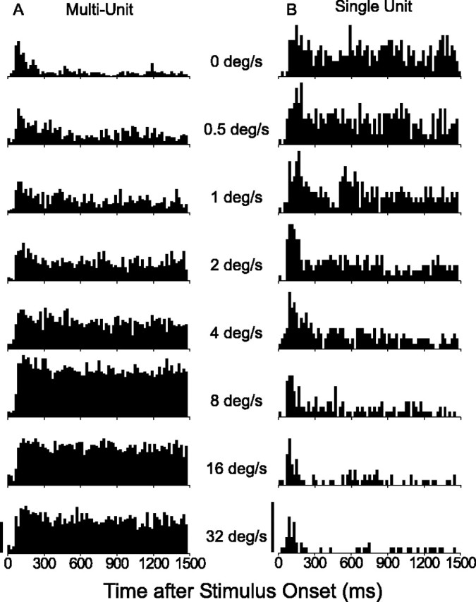
Time course of responses to stimuli of varying speeds for two MT units. A, PSTHs for an MT multiunit tested with preferred direction of motion at several speeds. Each PSTH is the average of responses to five stimulus repetitions. Note that responses to stationary and slow-moving stimuli are transient, whereas responses to fast-moving stimuli are strong and sustained. Calibration, 300 spikes/sec. B, PSTHs for a single unit that shows the opposite pattern of behavior. Responses to stationary and slow-moving stimuli are robust and sustained, whereas responses to fast-moving dots are weak and transient. Calibration, 50 spikes/sec.

Figure 8A shows summary data for the population of all of the multiunit recordings. Dashed curves show the average PSTH in response to dots moving at the preferred speed of each neuron; solid curves show the average PSTH for stationary dots. Thick curves were derived by averaging across units with strong responses to stationary stimuli (SMRR > 0.33); thin curves give average PSTHs for units with an SMRR of <0.33. For the latter group, responses to dots moving at the preferred speed are strong and sustained (thin dashed curve), whereas responses to stationary dots (thin solid curve) are transient and decay almost to spontaneous activity levels (zero response on this normalized scale) during the trial epoch. For the population with an SMRR of >0.33, responses to stationary dots (thick solid curve) have an initial transient followed by a substantial sustained component that remains well above the spontaneous activity level.

A very similar pattern of responses is shown in Figure 8B for the population of single-unit recordings, although the population PSTHs are a bit noisier because of the smaller sample size and weaker responses. Again, note the sustained responses to stationary stimuli for neurons with an SMRR of >0.33. Overall, it is clear that many MT units exhibit sustained responses to stationary stimuli throughout the 1.5 sec viewing period. We have no data to suggest whether or not this sustained component of response would decay to zero over a longer time period.

Dynamics of disparity selectivity

Given that responses to stationary stimuli (and, to a lesser extent, moving stimuli) exhibit a transient peak followed by a sustained component, we asked how disparity selectivity varies during the time course of the response. Is disparity selectivity present in the earliest responses of the neurons, or does it emerge later in time? And how does disparity selectivity decay with time in the latter stages of the response? To address these issues, we constructed disparity tuning curves from responses within a 40 msec time window, and we slid this window along the time course of the response in 10 msec increments. The resultant series of disparity tuning curves as a function of time was stacked up and plotted as a contour map. Figure 9A shows a disparity-time map for an example of a multiunit; this map was measured using stimuli moving at the preferred speed (7.3 deg/sec). Figure 9B shows the corresponding disparity-time map for stationary stimuli. In both cases, it can be seen that the earliest responses are disparity selective, and that the preferred disparity remains approximately constant throughout the response epoch.

Figure 9.

Dynamics of disparity selectivity for an example of an MT multiunit. A, Disparity-time map for responses to moving dots. A disparity tuning curve was constructed from responses in a 40 msec time window, and this time window was moved in 10 msec increments along the time course of the neural response. This produced a series of 100 disparity tuning curves, which were stacked together and plotted as a contour map (firing rate is color coded). B, Disparity-time map for responses of the same multiunit to stationary dots. C, Quantitative summary of the disparity-time data in A and B. From each of the 100 disparity tuning curves, two parameters were extracted: response at the preferred disparity and DDI. Black curves show the preferred response plotted against time for moving (solid) and stationary (dashed) stimuli. Analogously, red curves show the DDI plotted against time (right vertical axis).

Figure 9C quantitatively compares the time course of response and disparity selectivity (assessed using the DDI) for this multiunit example. Response time courses were computed as vertical cross-sections through the disparity-time maps at the preferred disparity of the neuron. The response to dots moving at the preferred speed (black solid line) is stronger and more sustained than the response to stationary dots (black dashed line), and both responses have a sharp onset with latency of ∼70 msec. Interestingly, the red curves show that DDI increases rapidly along with the response, and DDI reaches peak values at approximately the same time as the response. The DDI for moving dots (red solid line) remains quite constant throughout the time course of the response, whereas the DDI for stationary dots (dashed red line) declines in the latter stages of the trial epoch. It is interesting to note that the DDIs for moving and stationary stimuli are quite similar over the first few hundred milliseconds of the response.

Figure 10A shows that this pattern of dynamics was found across the population of 60 multiunit recordings with significant disparity tuning. Responses to moving and stationary dots (solid and dashed black lines, respectively) diverged shortly after peaking at ∼90 msec poststimulus. In contrast, DDI values for moving and stationary dots (red curves) remained at similar levels during the first 200 msec of the response; only later did DDI values for stationary dots drop markedly. A similar pattern of results can be seen for the population of 33 disparity-selective single units in Figure 10B.

Figure 10.

Population summary of response and disparity tuning dynamics. A, Population response (to the preferred disparity) and DDI as a function of time for the 60 of 76 multiunits with significant disparity tuning (ANOVA; p < 0.05). Data are in the same format as Figure 9C, except that the response curves for each unit were normalized (to a peak of 1.0) before averaging. DDI curves were simply averaged across units. B, Response and DDI as a function of time for the population of (33 of 42) MT single units with significant disparity tuning for both moving and stationary stimuli.

Figure 5C shows that DDI values are considerably lower for stationary stimuli when averaged over the entire 1.5 sec stimulus epoch. In contrast, Figure 10 shows that there is much less difference in DDI values between moving and stationary stimuli over the first few hundred milliseconds of the response. (Note that the absolute values of DDI in the two figures should not be compared because of the different analysis time windows.) Given that saccades typically occur every few hundred milliseconds in normal vision, MT neurons can signal disparity for static scenes with almost as much fidelity as they do for scenes that contain moving objects.

Can responses to stationary stimuli be explained by monitor refresh?

In using the term “stationary” to describe our stimuli, we ignored the fact that random-dot patterns were actually flickering at the refresh rate of the monitor (100 Hz). Because the response of magnocellular neurons in the lateral geniculate nucleus can be modulated at very high temporal frequencies (Derrington and Lennie, 1984; Hawken et al., 1996), we were concerned that some MT neurons might be entrained to the 100 Hz monitor refresh. If responses are periodically modulated at the refresh rate, this might account for the robust responses to stationary dots exhibited by many MT units.

To address this possibility, we computed an autocorrelogram of the responses to stationary stimuli for each MT unit (Wollman and Palmer, 1995). Figure 11A shows the autocorrelogram for the single unit shown previously in Figures 2, E and F, and 7B. There is a sharp dip in the autocorrelogram on either side of the central bin, reflecting the refractory period of the neuron. If this neuron were entrained to the 100 Hz refresh of the monitor, there should be repetitive peaks with a period of 10 msec in the auto-correlogram, but no such peaks are observed. To quantify this, we computed the power spectrum of the unit by Fourier transforming the autocorrelogram. As seen in Figure 10B, there is no peak in the power spectrum at 100 Hz.

Figure 11.

Responses to stationary stimuli are not driven by monitor refresh. A, Autocorrelogram of the spike train for a single unit that preferred stationary stimuli (same cell as in Fig. 2 E, F). B, Power spectrum of the same spike train (Fourier transform of the autocorrelogram). If response was entrained to the refresh of the monitor, there should be a peak at 100 Hz. C, For each MT unit in our sample, SMRR is plotted as a function of the power ratio (P100/Pflanks), which is defined as the power in the spike train at 100 Hz (P100) divided by the average power in the frequency ranges of 50-80 and 120-150 Hz (Pflanks). If strong responses to stationary dots were driven by monitor flicker, there should be a positive correlation in this scatter plot.

For each MT unit, we divided the power at 100 Hz (P100) by the average power in two flanking frequency bands: 50-80 and 120-150 Hz (Pflanks). Figure 11C shows the SMRR plotted against this power ratio (P100/Pflanks) for all of the MT units in our sample. We found no correlation between these variables (ANCOVA within-cells regression, r = 0.04; p = 0.67), indicating that strong responses to stationary stimuli were not attributable to periodic response modulations at the refresh rate of the monitor. Note also that most values of P100/Pflanks are close to unity, indicating the general lack of any peaks in the power spectrum at 100 Hz. This result also makes sense in terms of our other findings. Neurons that respond well to 100 Hz flicker would be expected to prefer high temporal frequencies and thus fast speeds. By this logic, one would expect to have the strongest responses to stationary stimuli for units that prefer fast speeds; we find just the opposite (Fig. 3A).

Can responses to stationary stimuli be explained by microsaccades?

Another possible explanation for the relatively strong responses that we observed to stationary stimuli involves microsaccades that take place within the monkey's fixation window. Bair and O'Keefe (1998) have shown that fixational microsaccades generally suppress the responses of MT neurons to near-optimal moving stimuli. They also noted, however, that microsaccades could elicit excitatory responses from neurons that were responding to stimuli that drove them weakly. If this were true for our stationary random-dot stimuli, then microsaccades could account for at least some of the responses that we observe. Microsaccades would not give rise to sustained discharges throughout a single trial, but could give this appearance when responses are averaged across multiple stimulus repetitions.

To assess the role of microsaccades in our data, we constructed a saccade-triggered average of the responses to stationary stimuli for each MT unit. For each trial, microsaccades were detected using a velocity criterion (see Materials and Methods) (Bair and O'Keefe, 1998; Leopold and Logothetis, 1998; Martinez-Conde et al., 2000). A portion of the spike train of the unit from 50 msec presaccade to 300 msec postsaccade was clipped out around the occurrence of each microsaccade, and these snippets were averaged across all of the saccades generated on trials in which stationary dots were presented. For the analyses presented here, microsaccades in all directions were included in the saccade-triggered averages, irrespective of the preferred direction of the neuron. Very similar results were obtained when we only included microsaccades having a direction within 45° of the preferred or null directions of the neuron.

Figure 12, A and B, shows data for an MT multiunit that preferred fast speeds. The saccade-triggered average (Fig. 12B) shows that this unit tended to fire a burst of spikes starting ∼70 msec after the occurrence of a microsaccade. Thus, microsaccades did contribute to the (weak) responses that this unit gave to stationary dots. In contrast, Figure 12, C and D, shows data for a single unit that gave its optimal response to stationary stimuli and exhibited no response to stimuli moving faster than ∼2 deg/sec. The saccade-triggered average for this neuron (Fig. 12D) shows a trough of suppression after microsaccades. This makes sense given that microsaccades typically have peak velocities in the range of 3-20 deg/sec (Martinez-Conde et al., 2000). Because the response of this MT neuron is suppressed below spontaneous activity in this range of speeds, small eye movements actually reduce the response of the neuron to stationary stimuli. Thus, microsaccades cannot underlie the strong responses to stationary stimuli exhibited by this neuron.

For each MT unit, we summarized the saccade-triggered average by computing the average value in a 50 msec window surrounding the peak or trough, and dividing this by the average value in a 50 msec window centered around time 0 (before any response to the saccade could occur). Figure 13A shows the SMRR plotted against this normalized amplitude of the saccade-triggered average for all of the units in our sample. If microsaccades were responsible for strong responses to stationary stimuli, one would expect to see a positive correlation in this scatter plot. In contrast, there is a highly significant (r = -0.47; p << 0.001) negative correlation, consistent with the idea that microsaccades hinder, rather than facilitate, responses to stationary dots.

Figure 13.

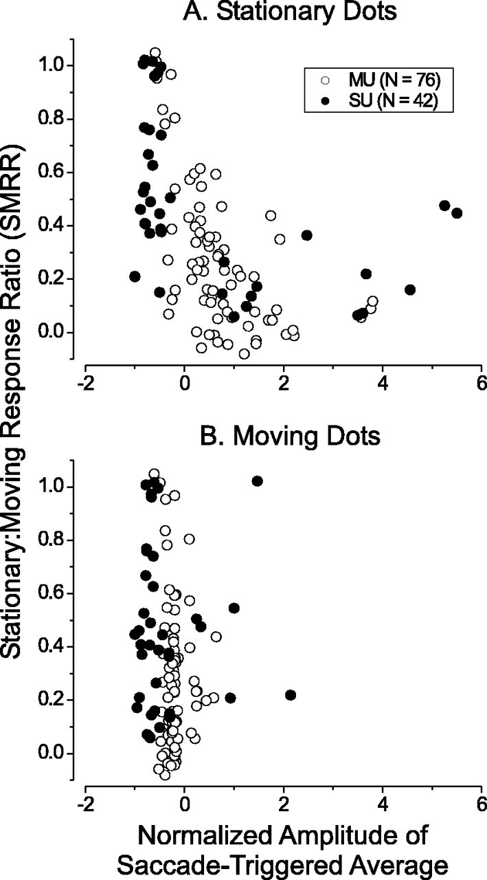
Microsaccades cannot account for responses to stationary stimuli. A, SMRR is plotted against the normalized amplitude of the saccade-triggered average for all of the units in our sample. For this plot, only saccades occurring during responses to stationary stimuli were used to compute the normalized amplitude of the saccade-triggered average. If responses to stationary stimuli were driven by microsaccades, one would expect a positive correlation in this plot. Instead, we find a significant negative correlation (r = -0.47; p << 0.001). B, SMRR is again plotted against the normalized amplitude of the saccade-triggered average; however, only saccades occurring during responses to moving stimuli (at the preferred speed) were included in this plot.

We also constructed saccade-triggered averages from responses to dots moving at the preferred speed, and Figure 13B shows summary data in the same form as A. For moving stimuli, the amplitude of the saccade-triggered average is generally negative, indicating that responses were suppressed after saccades. This is consistent with the findings of Bair and O'Keefe (1998).

Even during the intervals between microsaccades, there is some retinal image motion because of slow drifts and small tremors of the eye (Ditchburn and Ginsborg, 1953; Steinman et al., 1973; Skavenski et al., 1975). Thus, although we referred to our stimuli as stationary, the random-dot patterns are not completely stabilized on the retina (in which case the visual image would fade) (Ditchburn and Ginsborg, 1952). We cannot evaluate whether slow drifts and small tremors contribute to the responses of MT neurons in our experiments, because it is very difficult to distinguish these movements from noise in the eye position signals. In any case, these slow miniature eye movements are a normal part of natural vision, so their impact would not affect our conclusions.

Discussion

We directly compared the fidelity with which MT neurons code binocular disparity in response to random-dot stereograms that were either stationary or moving. Our findings can be summarized as four major points. First, many MT neurons give robust responses to stationary stimuli, and neurons that prefer slower speeds typically exhibit a strong sustained (i.e., tonic) discharge in the absence of stimulus motion. The striking examples of MT units (both single units and multiunit clusters) that prefer stationary stimuli appear to simply reflect a continuum of speed preferences that includes zero speed. Second, for most MT units, disparity tuning curves measured with stationary and moving stimuli have identical shapes. The main effect of adding optimal-velocity motion to the stimulus is an overall multiplicative scaling of the tuning curve by a factor of 2 on average. Third, across the entire 1.5 sec stimulus epoch, MT units have significantly lower discriminability for disparity when tested with stationary versus moving stimuli. However, discriminability is much more similar for moving and stationary stimuli during the first 200 msec of the response. Thus, in a typical time interval between saccades, MT neurons provide reliable disparity signals. Fourth, strong sustained responses to stationary stimuli cannot be explained by either monitor refresh or microsaccades. In fact, microsaccades typically suppress the responses of MT units that respond strongly to stationary stimuli.

Overall, our findings suggest that MT can contribute to depth perception during the viewing of static scenes. This view is supported by our previous finding that microstimulation of MT biased depth judgments when monkeys viewed stationary random-dot stereograms (DeAngelis et al., 1998). However, that result could have arisen because microstimulation produced a perception of both motion and depth, not simply depth. Also, stimulus refresh was substantially slower in those experiments, and sufficient data were not collected to properly analyze the effects of microsaccades. The present results show that MT neurons carry reliable disparity information about stationary stimuli, consistent with the microstimulation result.

Although we described our stationary stimuli as lacking motion, it is important to note that the onset of these flashed stimuli contains motion energy in all directions. Thus, it is not surprising that motion-selective neurons would give a substantial transient response to these stimuli. Notably, however, MT neurons with the strongest responses to stationary stimuli tend to have the largest tonic response components (e.g., the neuron of Figs. 2E,7B). Clearly, the time course of the response of these MT neurons does not simply follow the time course of motion energy in the stimulus.

Our results do not diminish the overwhelming evidence that MT is crucial for motion perception (for review, see Albright, 1993; Parker and Newsome, 1998). Rather, we suggest that the roles of MT in vision are not simply limited to the analysis of moving images. Our stimulus paradigm roughly approximates the situation in which a subject, whose head is still, makes saccadic eye movements around a stationary environment, thus abruptly introducing new patches of the visual image into the receptive fields of MT neurons every few hundred milliseconds. The main difference between our flashed stimuli (during fixation) and natural scanning of a scene is that saccades present a new patch of the image to neurons immediately after a brief pulse of very fast retinal image motion. We did not mimic these saccade-related bursts of motion in our stimulus set.

However, a recent study has examined the effects of large saccades on the responses of MT neurons to retinal image motion (Thiele et al., 2002). For 17% of MT neurons, responses were suppressed strongly by saccades. The visual responses of 34% of MT neurons were unaffected by saccades, and the remaining ∼50% of neurons were suppressed by saccades in some directions but facilitated by saccades in other directions. Thus, the overall average effect of saccades on MT responses was small. The impact of these effects on our conclusions is not clear, because the data of Thiele et al. (2002) do not indicate how saccadic effects depend on the speed preferences of MT neurons, but it seems likely that the impact would be small. Suppression could reduce the early transient response of some MT neurons to both moving and stationary stimuli, but it would not eliminate the tonic responses to stationary stimuli that we observed (Fig. 7B). Thus, although this issue deserves additional study, we think that our results have considerable bearing on the role of MT in natural three-dimensional (3D) vision.

Comparison to V1

Muller et al. (2001) have recently compared the responses of V1 neurons to moving and stationary grating stimuli. Many of our analyses are similar to theirs, and the results from V1 and MT are quite comparable. In response to stationary gratings flashed for 1.25 sec, most V1 neurons give a brisk transient response followed by a sustained response that averages 20% of the peak transient response [Muller et al. (2001), their Fig. 2] (for a similar result, see also Albrecht et al., 2002). From our Figures 8 and 10, it can be seen that the average responses of our MT neurons to stationary stimuli follow a very similar pattern. Muller et al. (2001) show that orientation tuning curves are nearly identical in shape for stationary and drifting gratings. They also show that the discriminability of V1 neurons for orientation is similar for stationary and drifting gratings during the initial 100-200 msec of the response, whereas discriminability is substantially higher for moving stimuli over longer periods of time. This comparison indicates that the relative strength and fidelity of responses to stationary and moving stimuli are similar for areas V1 and MT.

Speed tuning

There is a large difference in the range of preferred speeds of MT neurons between our study and some previous studies. For our population of single units, two-thirds (213 of 319) have preferred speeds of <10 deg/sec. In contrast, only ∼15-25% of MT units had preferred speeds of <10 deg/sec in three previous studies (Maunsell and Van Essen, 1983a; Mikami et al., 1986; Cheng et al., 1994). Ranges of eccentricities were approximately similar in all of the studies, and there appears to be no difference in speed tuning between studies in alert and anesthetized animals (Mikami et al., 1986). One major difference is that these previous studies used moving-bar stimuli, whereas we used drifting random-dot patterns. With bars, different portions of the receptive field are stimulated sequentially, whereas the entire receptive field is stimulated simultaneously in our experiments. As the speed of a bar increases, the time it takes to traverse the receptive field decreases proportionally. For very fast speeds, the bar stimulus will essentially be a brief flash in the MT receptive field. Thus, the method of data analysis may be critical for characterizing responses to bar stimuli. All of the above studies computed average firing rates over a variable length analysis window that changed with stimulus speed. In contrast, Lagae et al. (1993) measured peak firing rates in response to moving bars and found a range of preferred speeds nearly identical to ours (Lagae et al., 1993, their Fig. 16C). Therefore, it seems that stimulus type and/or analysis method may account for a large portion of the difference between our study and others.

Given that our range of speeds was limited to a maximum of 32 deg/sec, it is nevertheless important to consider the extent to which this may have biased our sample. In a recent study, Liu and Newsome (2003) measured the speed tuning of a large, unbiased sample of multiunits in MT using random-dot stimuli with a maximum speed of ∼80 deg/sec. They found ∼20-25% of sites with speed preferences outside of the range we used. Similarly, Churchland and Lisberger (2001) measured the speed tuning of MT single units using random-dot stimuli with a larger range of speeds than ours and found <20% of neurons with speed preferences of >32 deg/sec. Thus, although our sample is somewhat biased toward slower speeds, this bias is sufficiently small that it does not affect our basic conclusions.

In summary, our results show that many MT neurons respond robustly to stationary stimuli and carry binocular disparity information with high fidelity, especially in the first 200 msec of the response. This finding suggests that MT conveys important visual information during typical intervals between saccadic eye movements, when the only retinal image motion is attributable to slow drifts and small tremors of the eye (Ditchburn and Ginsborg, 1953; Steinman et al., 1973; Skavenski et al., 1975). Although we only investigated the coding of horizontal disparities, MT may also carry other types of information regarding stationary stimuli. For example, we recently found that many MT neurons signal the 3D orientation of planar surfaces defined by disparity gradients, and that this selectivity remains when coherent motion is removed from the visual stimulus (Nguyenkim and DeAngelis, 2003). MT neurons may therefore play a substantial role in specifying the 3D structure of the scene regardless of whether there is visual motion in their receptive fields.

References

- Albrecht DG, Geisler WS, Frazor RA, Crane AM ( 2002) Visual cortex neurons of monkeys and cats: temporal dynamics of the contrast response function. J Neurophysiol 88: 888-913. [DOI] [PubMed] [Google Scholar]
- Albright TD ( 1984) Direction and orientation selectivity of neurons in visual area MT of the macaque. J Neurophysiol 52: 1106-1130. [DOI] [PubMed] [Google Scholar]
- Albright TD ( 1993) Cortical processing of visual motion. Rev Oculomot Res 5: 177-201. [PubMed] [Google Scholar]
- Bair W, O'Keefe LP ( 1998) The influence of fixational eye movements on the response of neurons in area MT of the macaque. Vis Neurosci 15: 779-786. [DOI] [PubMed] [Google Scholar]
- Britten KH, Shadlen MN, Newsome WT, Movshon JA ( 1992) The analysis of visual motion: a comparison of neuronal and psychophysical performance. J Neurosci 12: 4745-4765. [DOI] [PMC free article] [PubMed] [Google Scholar]
- Cheng K, Hasegawa T, Saleem KS, Tanaka K ( 1994) Comparison of neuronal selectivity for stimulus speed, length, and contrast in the prestriate visual cortical areas V4 and MT of the macaque monkey. J Neurophysiol 71: 2269-2280. [DOI] [PubMed] [Google Scholar]
- Churchland MM, Lisberger SG ( 2001) Shifts in the population response in the middle temporal visual area parallel perceptual and motor illusions produced by apparent motion. J Neurosci 21: 9387-9402. [DOI] [PMC free article] [PubMed] [Google Scholar]
- Cumming BG, Parker AJ ( 1999) Binocular neurons in V1 of awake monkeys are selective for absolute, not relative, disparity. J Neurosci 19: 5602-5618. [DOI] [PMC free article] [PubMed] [Google Scholar]
- DeAngelis GC, Newsome WT ( 1999) Organization of disparity-selective neurons in macaque area MT. J Neurosci 19: 1398-1415. [DOI] [PMC free article] [PubMed] [Google Scholar]
- DeAngelis GC, Uka T ( 2003) Coding of horizontal disparity and velocity by MT neurons in the alert macaque. J Neurophysiol 89: 1094-1111. [DOI] [PubMed] [Google Scholar]
- DeAngelis GC, Cumming BG, Newsome WT ( 1998) Cortical area MT and the perception of stereoscopic depth. Nature 394: 677-680. [DOI] [PubMed] [Google Scholar]
- Derrington AM, Lennie P ( 1984) Spatial and temporal contrast sensitivities of neurones in lateral geniculate nucleus of macaque. J Physiol (Lond) 357: 219-240. [DOI] [PMC free article] [PubMed] [Google Scholar]
- Ditchburn RW, Ginsborg BL ( 1952) Vision with a stabilized retinal image. Nature 170: 3637-3640. [DOI] [PubMed] [Google Scholar]
- Ditchburn RW, Ginsborg BL ( 1953) Involuntary eye movements during fixation. J Physiol (Lond) 119: 1-17. [DOI] [PMC free article] [PubMed] [Google Scholar]
- Draper NR, Smith H ( 1966) Advanced regression analysis. New York: Wiley.
- Felleman DJ, Van Essen DC ( 1991) Distributed hierarchical processing in the primate cerebral cortex. Cereb Cortex 1: 1-47. [DOI] [PubMed] [Google Scholar]
- Groh JM, Born RT, Newsome WT ( 1997) How is a sensory map read out? Effects of microstimulation in visual area MT on saccades and smooth pursuit eye movements. J Neurosci 17: 4312-4330. [DOI] [PMC free article] [PubMed] [Google Scholar]
- Hawken MJ, Shapley RM, Grosof DH ( 1996) Temporal-frequency selectivity in monkey visual cortex. Vis Neurosci 13: 477-492. [DOI] [PubMed] [Google Scholar]
- Komatsu H, Wurtz RH ( 1989) Modulation of pursuit eye movements by stimulation of cortical areas MT and MST. J Neurophysiol 62: 31-47. [DOI] [PubMed] [Google Scholar]
- Lagae L, Raiguel S, Orban GA ( 1993) Speed and direction selectivity of macaque middle temporal neurons. J Neurophysiol 69: 19-39. [DOI] [PubMed] [Google Scholar]
- Leopold DA, Logothetis NK ( 1998) Microsaccades differentially modulate neural activity in the striate and extrastriate visual cortex. Exp Brain Res 123: 341-345. [DOI] [PubMed] [Google Scholar]
- Lewis JW, Van Essen DC ( 2000) Corticocortical connections of visual, sensorimotor, and multimodal processing areas in the parietal lobe of the macaque monkey. J Comp Neurol 428: 112-137. [DOI] [PubMed] [Google Scholar]
- Lisberger SG, Movshon JA ( 1999) Visual motion analysis for pursuit eye movements in area MT of macaque monkeys. J Neurosci 19: 2224-2246. [DOI] [PMC free article] [PubMed] [Google Scholar]
- Liu J, Newsome WT ( 2003) Functional organization of speed tuned neurons in visual area MT. J Neurophysiol 89: 246-256. [DOI] [PubMed] [Google Scholar]
- Marcar VL, Xiao DK, Raiguel SE, Maes H, Orban GA ( 1995) Processing of kinetically defined boundaries in the cortical motion area MT of the macaque monkey. J Neurophysiol 74: 1258-1270. [DOI] [PubMed] [Google Scholar]
- Martinez-Conde S, Macknik SL, Hubel DH ( 2000) Microsaccadic eye movements and firing of single cells in the striate cortex of macaque monkeys. Nat Neurosci 3: 251-258. [DOI] [PubMed] [Google Scholar]
- Maunsell JHR, Newsome WT ( 1987) Visual processing in monkey extrastriate cortex. Annu Rev Neurosci 10: 363-401. [DOI] [PubMed] [Google Scholar]
- Maunsell JHR, Van Essen DC ( 1983a) Functional properties of neurons in middle temporal visual area of the macaque monkey. I. Selectivity for stimulus direction, speed, and orientation. J Neurophysiol 49: 1127-1147. [DOI] [PubMed] [Google Scholar]
- Maunsell JH, Van Essen DC ( 1983b) Functional properties of neurons in middle temporal visual area of the macaque monkey. II. Binocular interactions and sensitivity to binocular disparity. J Neurophysiol 49: 1148-1167. [DOI] [PubMed] [Google Scholar]
- Mikami A, Newsome WT, Wurtz RH ( 1986) Motion selectivity in macaque visual cortex. I. Mechanisms of direction and speed selectivity in extra-striate area MT. J Neurophysiol 55: 1308-1327. [DOI] [PubMed] [Google Scholar]
- Muller JR, Metha AB, Krauskopf J, Lennie P ( 2001) Information conveyed by onset transients in responses of striate cortical neurons. J Neurosci 21: 6978-6990. [DOI] [PMC free article] [PubMed] [Google Scholar]
- Newsome WT, Wurtz RH, Dursteler MR, Mikami A ( 1985) Deficits in visual motion processing following ibotenic acid lesions of the middle temporal visual area of the macaque monkey. J Neurosci 5: 825-840. [DOI] [PMC free article] [PubMed] [Google Scholar]
- Nguyenkim JD, DeAngelis GC ( 2003) Disparity-based coding of three-dimensional surface orientation by macaque middle temporal neurons. J Neurosci 23: 7117-7128. [DOI] [PMC free article] [PubMed] [Google Scholar]
- Parker AJ, Newsome WT ( 1998) Sense and the single neuron: probing the physiology of perception. Annu Rev Neurosci 21: 227-277. [DOI] [PubMed] [Google Scholar]
- Prince SJ, Pointon AD, Cumming BG, Parker AJ ( 2002) Quantitative analysis of the responses of V1 neurons to horizontal disparity in dynamic random-dot stereograms. J Neurophysiol 87: 191-208. [DOI] [PubMed] [Google Scholar]
- Rodman HR, Albright TD ( 1987) Coding of visual stimulus velocity in area MT of the macaque. Vision Res 27: 2035-2048. [DOI] [PubMed] [Google Scholar]
- Schiller PH, Lee K ( 1994) The effects of lateral geniculate nucleus, area V4, and middle temporal (MT) lesions on visually guided eye movements. Vis Neurosci 11: 229-241. [DOI] [PubMed] [Google Scholar]
- Skavenski AA, Robinson DA, Steinman RM, Timberlake GT ( 1975) Miniature eye movements of fixation in rhesus monkey. Vision Res 15: 1269-1273. [DOI] [PubMed] [Google Scholar]
- Snowden RJ, Treue S, Andersen RA ( 1992) The response of neurons in areas V1 and MT of the alert rhesus monkey to moving random dot patterns. Exp Brain Res 88: 389-400. [DOI] [PubMed] [Google Scholar]
- Steinman RM, Haddad GM, Skavenski AA, Wyman D ( 1973) Miniature eye movement. Science 181: 810-819. [DOI] [PubMed] [Google Scholar]
- Thiele A, Henning P, Kubischik M, Hoffmann KP ( 2002) Neural mechanisms of saccadic suppression. Science 295: 2460-2462. [DOI] [PubMed] [Google Scholar]
- Van Essen DC, Gallant JL ( 1994) Neural mechanisms of form and motion processing in the primate visual system. Neuron 13: 1-10. [DOI] [PubMed] [Google Scholar]
- Wollman DE, Palmer LA ( 1995) Phase locking of neuronal responses to the vertical refresh of computer display monitors in cat lateral geniculate nucleus and striate cortex. J Neurosci Methods 60: 107-113. [DOI] [PubMed] [Google Scholar]
- Zeki SM ( 1974) Functional organization of a visual area in the posterior bank of the superior temporal sulcus of the rhesus monkey. J Physiol (Lond) 236: 549-573. [DOI] [PMC free article] [PubMed] [Google Scholar]