

Abstract
Statistical analysis of natural sounds and speech reveals logarithmically distributed spectrotemporal modulations that can cover several orders of magnitude. By contrast, most artificial stimuli used to probe auditory function, including pure tones and white noise, have linearly distributed amplitude fluctuations with a limited average dynamic range. Here we explore whether the operating range of the auditory system is physically matched to the statistical structure of natural sounds. We recorded single-unit and multi-unit neuronal activity from the central nucleus of the cat inferior colliculus (ICC) in response to dynamic spectrotemporal sound sequences to determine whether ICC neurons respond preferentially to linear or logarithmic spectrotemporal amplitudes. We varied the intensity, dynamic range, and contrast statistics of these sounds to mimic those of natural and artificial stimuli. ICC neurons exhibited monotonic and nonmonotonic contrast dependencies with increasing dynamic range that were independent of the stimulus intensity. Midbrain neurons had higher firing rates and higher receptive field energies and showed a net improvement in spectrotemporal encoding ability for logarithmic stimuli, with an increase in the mutual information rate of ∼50% over linear amplitude sounds. This efficient use of logarithmic spectrotemporal modulations by auditory midbrain neurons reflects a neural adaptation to structural regularities in natural sounds and likely underlies human perceptual abilities.
Keywords: contrast, modulation depth, inferior colliculus, spectrotemporal, reverse correlation, mutual information, natural sounds
Introduction
A central hypothesis of sensory coding asserts that sensory systems efficiently make use of statistical structure inherent in natural signals. The possibility that sensory systems are adapted for encoding natural signals has been a topic of discussion since the early work of Barlow (1953, 1961). Recent work has revealed that natural visual (Ruderman and Bialek, 1994; Dong and Atick, 1995; Ruderman, 1997) and acoustic signals (Voss and Clarke, 1975; Attias and Schreiner, 1998; Nelken et al., 1999; Lewicki 2002) show robust statistical properties such as scale invariant contrast statistics and 1/f modulation spectrum. Although numerous studies have looked at these statistical characteristics of natural signals, only a few studies have addressed how such statistics can be used for efficient sensory coding (Rieke and Bodnar, 1995; Dan et al., 1996; Attias and Schreiner, 1998; Nelken et al., 1999; Stanley et al., 1999). Direct application of information theoretic approaches has revealed that sensory neurons respond most efficiently to sensory signals with natural statistics, although the exact mechanisms enabling such efficient processing have not been established.
In natural vision and hearing, our senses are exposed to stimuli that span many orders of magnitude in their mean and instantaneous intensities. Measurements of the spectral, spatial, or temporal fluctuations in the local energy of the sensory signal are typically represented by the modulation index for sounds or by the contrast for visual images. Both of these measures rely on the peak-to-peak amplitude excursion of the sensory signal as the relevant signal parameter and do not fully account for the intermediate amplitudes of the sensory waveform. Temporal modulations in natural sounds and spatial fluctuations in natural scenes, however, cover several orders of magnitude and therefore are represented best by the log-amplitude transform (Ruderman and Bialek, 1994; Attias and Schreiner, 1998).
Spatial and temporal energy gradations represent much of the information-bearing components of sensory signals, and we therefore expect that sensory systems efficiently make use of spectrotemporal information found in natural sounds and spatiotemporal information found in natural scenes. Considering the rules for scaling in natural sounds and visual scenes, and the logarithmic Weber's law scaling for intensity and luminance discrimination (Weber 1834; Fechner, 1860; Miller, 1947; Harris, 1963; Jesteadt and Wier, 1977; Florentine et al., 1987), one hypothesis is that sensory systems are attuned to logarithmic modulations. We therefore would like to determine whether the log-transform signal expressed in units of decibels, 20 · log10 (s(t)), is potentially more important than the corresponding linear amplitude auditory signal, s(t).
Numerous studies have addressed the neuronal representation of time-varying sounds, although these have traditionally focused on linear amplitude excursions. Studies on sinusoidal amplitude modulation (AM) have demonstrated that phase-locking sensitivity improves with increasing modulation index in the inferior colliculus (ICC) and neuronal firing rates increase monotonically, although these can saturate with as little as 20% modulation index (Rees and Moller, 1983; Krishna and Semple, 2000). There is some evidence, however, indicating that neurons are also sensitive to the higher-order moments in temporally modulated amplitudes in acoustic signals, even at near 100% modulation depth where firing rates appear to be fully saturated. First, auditory neurons in the cochlea and throughout the entire auditory pathway are exceptionally sensitivity to the velocity and acceleration profiles of temporally ramped stimuli (Heil, 1997a,b; Heil and Irvine, 1997). First-spike timing precision and trial-to-trial reproducibility improve with increasing velocity or acceleration of the temporal acoustic waveform. Time reversal of ramped auditory stimuli produces a shift in the perceived quality and intensity (Irino and Patterson, 1996; Akeroyd and Patterson, 1997) that is reflected in the response of primary auditory cortex neurons (Lu et al., 2001), although these sounds have identical peak-to-peak contrast and energy spectrum. Finally, neurons in the auditory midbrain are sensitive to higher-order moments of modulation waveform, such as the skewness and kurtosis, and appear to respond preferentially to synthetic sounds with naturally matched temporal modulations (Attias and Schreiner, 1998). These studies provide evidence that the entire distribution of amplitudes is critical for the neuronal representation, and the peak-to-peak values alone do not account for a significant fraction of observed neuronal responses.
Evidence for the relevance of the log-transform amplitude modulations comes from neurophysiology studies on the representation of sound intensity. Peripheral and central auditory neurons typically respond with an operating range of 30-50 dB and can show monotonic or nonmonotonic rate-level dependencies in central stations (Evans and Whitfield, 1964; Palmer and Evans, 1982; Ehret and Merzenich, 1988; Eggermont, 1989; Sutter and Schreiner, 1995). Psychophysical evidence further suggests that loudness perception and just-noticeable difference limens for intensity discrimination follow logarithmic (e.g., Weber's Law) relationships (Miller, 1947; Stevens, 1957; Harris, 1963; Jesteadt and Wier, 1977; Florentine et al., 1987). It is therefore likely that the operating range of auditory neurons is also used to process fine spectrotemporal information found in natural sounds.
We tested whether the operating range of single neurons is suited for encoding spectrotemporal information found in natural signals by comparing the neuronal representation of log-amplitude spectrotemporal modulations, 20 · log10(S(t,f)) (units of decibels), with the corresponding linear amplitude spectrotemporal excursions, S(t,f). Statistical analysis of natural sounds shows that natural signals follow logarithmic scaling laws, having an effective dynamic range that is comparable with the intensity operating range of single neurons for pure tones. Neuronal activity in the cat ICC to logarithmic rippled noise (RN) signals (Escabí and Schreiner, 2002) was marked by improvement in spectrotemporal processing ability, including higher spike rates and increased mutual information rates. These findings suggest that the operating range of the auditory system is matched to the spectrotemporal amplitude statistics of natural sensory stimuli.
Materials and Methods
Natural sound analysis. We studied the spectrotemporal modulations in natural sounds to identify potential differences among various classes of natural sounds and to determine whether neurons in the CNS preferentially encode signals with similar statistical properties. The ensemble of natural sounds included animal vocalizations (64.6 min), continuous running speech (74.0 min), and environmental sounds (51.1 min). As a control, white noise (10 min) was also analyzed using identical analysis procedure. No attempt was made to limit the sounds to any particular subcategory or species. All vocalizations and environmental sound were obtained from commercially available compact disk media from the Macaulay Library of Natural Sounds at Cornell University (Storm, 1994a,b; Emmons et al., 1997). Human speech was obtained from a radio broadcast reproduction of the William Shakespeare play Hamlet (Shakespeare, 1992). All sounds were sampled at a rate of 44.1 kHz and 16-bit resolution.
Sounds were initially decomposed by a bank of tonotopically arranged filters into a spectrotemporal representation that mimics the spectral decomposition performed by the cochlea. Filter center frequencies were arranged according to the frequency position function of the cochlea over a range covering 250 Hz to 14 kHz, and filter bandwidths were selected according to the perceptual critical bandwidths (Greenwood, 1990). Sounds waveforms were decomposed according to:
 |
1 |
where hk(t) is the impulse response of the k-th filter channel centered about the frequency fk, * is shorthand for the convolution operator, and s(t) is the sound waveform. Spectrotemporally compact B-spline filters (Roark and Escabí, 1999) were chosen for this analysis to minimize cross talk across adjacent filter channels and across separate time instants. For the purpose of the statistical analysis, filter bandwidths overlapped by 50%. To increase the display resolution in Figure 1, however, filters were overlapped by 90%.
Figure 1.
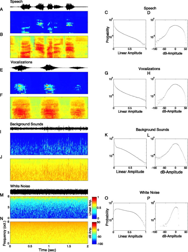
Analysis of the spectrotemporal contrast statistics of natural sounds and white noise. Cochlear model output representation showing the spectrotemporal modulations of a short segment of human conversational speech (A, B), animal vocalizations (E, F), environment background sounds (running water) (I, J), and white noise (M, N). Color scales are expressed either as a linear amplitude spectrotemporal modulation (normalized for a maximum value of 1) (A, E, I, M) or as the corresponding log-amplitude spectrotemporal modulation pattern (zero mean) expressed in units of decibels (B, F, J, N). The corresponding acoustic sound pressure waveforms are shown for each sound segment above each spectrotemporal envelope in black. The log-transformed spectrotemporal envelope expands the visible dynamic range of the stimulus, revealing detail that is not visible in the linear amplitude spectrotemporal modulation envelope. For each of the sound ensembles, the amplitude values from each spectrotemporal envelope were converted into a probability histogram for both the linear (C, G, K, O) and log-transform spectrotemporal envelope (D, H, L, P). The linear amplitude distribution of all natural sounds (C, G, K) shows a exponential-like distribution in which most of the stimulus components fall at low amplitude values. By comparison, the linear amplitude distribution of white noise (O) covers much of the linear amplitude dimension. The corresponding log-amplitude distributions exhibit a bell-shaped profile in which speech had the broadest dynamic range (D) and white noise covered the narrowest range of amplitude values (P).
The temporal waveform at the output of each filter was processed to extract the relative temporal modulations in each filter channel. First, the time-waveform of the k-th filter output, sk(t), was decomposed into a temporal envelope:
 |
2 |
where H[·] is the Hilbert transform operator (Hilbert, 1912) and ek(t) is the temporal modulation envelope of the k-th frequency channel centered about a frequency of fk. Next, the temporal envelope of each filter channel was low-pass filtered to limit the modulations across each filter channel to a maximum rate of 100 Hz:
 |
3 |
where h100 (t) is the impulse response of a low-pass B-spline filter with cutoff frequency of 100 Hz and Sk(t) is the band-limited temporal modulation envelope centered about a frequency of fk. This filtering was necessary so that all spectral channels have identical modulation bandwidths. A modulation bandwidth of 100 Hz was chosen because the cochleotopic filter bank decomposition contained filter bandwidths of ∼100 Hz at frequencies below 1 kHz, and therefore the outputs for these frequency channels did not contain modulations above 100 Hz. We treat Sk(t) as a two-dimensional function S(t,fk), the spectrotemporal envelope, which displays the energy modulations of each natural sound waveform as a function of frequency and time.
We were interested in the average statistical characteristics of the relative spectrotemporal fluctuations of each signal. After the filter bank decomposition, the envelopes were therefore rescaled according to a linear amplitude convention:
 |
4 |
where SMax = max[S(t,fk)] is the maximum amplitude value of the spectrotemporal envelope, S(t,fk). This rescaling limits the maximum amplitude of the spectrotemporal modulations to 1, consistent with traditional definitions of the analytic modulation signal (Hilbert, 1912). The rescaling also preserves the relative excursions and spectrotemporal interrelationships across each frequency band.
Psychophysics of loudness perception and intensity discrimination suggest that relative amplitude fluctuations described using decibel amplitude may be a more appropriate representation of the acoustic waveform. We therefore also considered a log-transform version of the spectrotemporal envelope:
 |
5 |
where μdB is the mean value of 20 log10 (S(t,fk)). This transformation removes the mean spectrotemporal level while preserving the variance and expresses the spectrotemporal envelope in units of decibels.
Analysis of the spectrotemporal envelope statistics consisted of measuring the amplitude distribution function for both the linear and decibel amplitude envelopes. Pixel values obtained from the spectrotemporal envelope were compounded into an amplitude distribution function, p[SLin] and p[SdB], where p[·] is the amplitude distribution function and SLin = SLin(t,fk) and SdB = SdB (t,fk) are shorthand for the linear and decibel spectrotemporal envelopes, respectively. Examples of the corresponding ensemble distributions for speech, vocalizations, background sounds, and white noise are illustrated in Figure 1. Additional analysis also consisted of estimating standard statistical measures directly from SLin and SdB (see Table 1). These included the modulation index, β = (SMax - SMin)/SMax, and the contrast, C = (SMax - SMin)/(SMax + SMin) as well as the waveform SDs, 90th percentile range, and skewness.
Table 1.
Summary statistics for the natural sound ensembles and white noise comparing the linear versus the log amplitude analysis
|
|
Linear amplitude |
Log amplitude (dB) |
||||||||||||
|---|---|---|---|---|---|---|---|---|---|---|---|---|---|---|
|
|
Mean (×10−3)
|
SD (×10−3)
|
Skewness
|
90th percentile range (×10−3)
|
Mean
|
SD (dB)
|
Skewness
|
90th percentile range (dB)
|
||||||
| Speech | 2.3 | 6.29 | 7.81 | 0-4.5 | 0 | 14.84 | 0.1001 | −28.4-20.6 | ||||||
| Vocalizations | 3.1 | 7.49 | 7.15 | 0-6.5 | 0 | 13.32 | 0.072 | −21.9-21.1 | ||||||
| Environment | 5.4 | 9.1 | 5.71 | 0-12.0 | 0 | 9.09 | −0.3866 | −14.5-15.5 | ||||||
| White noise
|
40.7
|
26.13
|
0.99
|
0-79.5
|
0
|
6.1
|
−0.48
|
−8.7-10.3
|
||||||
Electrophysiology. A detailed account of our experimental methods has been reported previously (Escabí and Schreiner, 2002). Briefly, cats (n = 4) were initially anesthetized with a mixture of ketamine HCl (10 mg/kg) and acepromazine (0.28 mg/kg, i.m.). After an intravenous infusion line was inserted, a surgical state of anesthesia was induced with ∼30 mg/kg Nembutal and maintained throughout the surgery with supplements. Body temperature was measured and maintained with a heating pad at ∼37.5°C. An incision was made in the intercartilaginous area of the trachea, and a tracheotomy tube was inserted. After a craniotomy was performed, the ICC was exposed by removing the overlying cerebrum and part of the bony tentorium using a dorsal approach. On completion of the surgery, the animal was maintained in an areflexive state of anesthesia via continuous infusion of ketamine (2-4 mg · kg-1 · hr-1) and diazepam (0.4-1 mg · kg-1 · hr-1) in lactated Ringer's solution (1-4 mg · kg-1 · hr-1). The state of the animal was monitored (heart rate, breathing rate, temperature, and reflexes) throughout the experiment, and the infusion rate was adjusted according to physiologic criteria. Every 12 hr the cat received an injection of dexamethasone (0.14 mg/kg, s.c.) and atropine (0.04 mg · kg-1 · d-1, s.c.). All surgical methods and experiment procedures followed National Institutes of Health and United States Department of Agriculture guidelines and were approved by the committee on animal research, University of California, San Francisco.
Data were obtained from single units (su) and multi-units (mu) in the ICC. One or two closely spaced parylene-coated tungsten microelectrodes (Microprobe Inc., Potomac, MD; 1-3 MΩ at 1 kHz) were advanced with a hydraulic microdrive (David Kopf Instruments, Tujunga, CA). Electrode penetration trajectories were at ∼20-30° relative to the sagittal plane and approximately orthogonal to the isofrequency band lamina. Action potential traces were recorded onto a digital audio tape (CDAT16; Cygnus Technologies, Delaware Water Gap, PA) at a sampling rate of 24.0 kHz (41.7 μsec resolution) for off-line analysis. Off-line analysis consisted of digital bandpass filtering (0.3-10 kHz) all spike trains and individually spike sorting the action potential traces using a Bayesian spike-sorting algorithm (Lewicki, 1994).
Acoustic stimuli. Our analysis of natural sounds suggests that spectrotemporal fluctuations in natural sounds have a broad dynamic range and that these are most appropriately described by the decibel amplitude variable. Therefore, we hypothesized that sensory neurons in the CNS should respond best to sounds that efficiently cover the decibel amplitude dimension.
One approach for testing this hypothesis is to compare the response of natural sounds with those of altered natural sounds. This approach may be limited by the high dimensionality and the correlations present in natural sounds that may prevent us from measuring true contrast effects. Although we currently know very little about the statistical properties of natural sounds, it is generally agreed that these are structurally complex and exhibit spectral and temporal correlations over a wide range of scales (Voss and Clarke, 1975; Attias and Schreiner, 1998; Theunissen et al., 2000). Therefore, modifying the contrast of a natural sound directly could potentially modify some alternate dependent variable. We therefore used synthetic stimuli with logarithmically matched and unmatched contrast statistics to study the efficiency of neuronal coding in the inferior colliculus.
The synthetic sounds consist of RN stimuli (Escabí and Schreiner, 2002) that are compatible with reverse correlation and can be used to estimate the spectrotemporal receptive field (STRF) of a neuron. These stimuli dynamically activate the sensory epithelium in the cochlea and allow us to estimate neuronal preferences in an unbiased manner. The spectrotemporal envelope of this stimulus is shown in Figure 2. It has noise-like properties with energy fluctuations that span a temporal modulation range of 0-350 Hz and spectral modulations from 0 to 4 cycles per octave. Signals were generated by modulating individual sinusoidal carriers of frequency, fk, and random phase, ϕk:
 |
6 |
over a range of 0.5-20 kHz by the stimulus spectrotemporal envelope S(t,Xk). Here Xk = log2 (fk/f0) is an octave frequency axis and the carrier spacing was set to ΔX = 0.0231 octaves.
Figure 2.
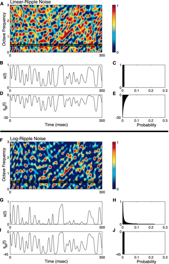
Spectrotemporal envelope and contrast statistics of the Lin- and Log-ripple noise test stimulus. The RN spectrotemporal envelope has random intensity modulations along the temporal and frequency stimulus dimensions (A, F). Log- and Lin-RN have identical spectrotemporal features and differ only in their amplitude statistics (A, F; both shown on a linear amplitude color scale). Temporal cross section of the Lin sound on a linear amplitude axis (B), Lin sound on a decibel axis (D), Log sound on a linear axis (G), and Log sound on a decibel axis (I). The amplitude distributions of each sound (Lin- and Log-RN) are shown, respectively (far right), on a linear (C and H, respectively) and decibel (E and J, respectively) amplitude axis. The Lin-RN follows a uniform linear amplitude distribution, whereas the Log-RN is uniformly distributed on a log-amplitude axis.
To address our initial hypothesis of which stimulus dimension is most important (linear or decibel amplitude), the amplitude statistics of the RN spectrotemporal envelope were designed either on a decibel or linear amplitude axis, without modifying the spectrotemporal content. First we created a generic RN spectrotemporal envelope, Sg(t,Xk), that was used to construct all of the sampled acoustic waveforms. From this we constructed five RN sounds that differed only in the contrast statistics of their envelope: sLin(t), s15(t), s30(t), s45(t), and s60(t). Subscripts denote the type of spectrotemporal contrast statistic: Lin designates an RN with linearly distributed amplitude statistics (see Fig. 2A-E). Numerical values designate the dynamic range (in decibels) for RN sounds with logarithmic-distributed (Log) contrast statistics (see Fig. 2F-J). The later sounds therefore had contrast statistics that could cover several orders of magnitude, as is evident for all natural sounds. Because sounds were constructed using an identical generic envelope (Sg(t,Xk)) by applying a nonlinear transformation, all sound sequences had identical spectrotemporal content and differed only in their contrast (amplitude) statistics.
The generic ripple noise envelope has uniformly distributed amplitude statistics in the interval 0-1. Decibel distributed sounds were constructed by applying the transformation:
 |
7 |
to the generic envelope, where M designates the dynamic range of the envelope in units of decibels (M assumes values of 15, 30, 45, or 60 dB). The decibel envelope for this sound, SdB(t,Xk) = 20 · log10(S(t,Xk)) = M · Sg(t,Xk) - M, has a uniform amplitude distribution in the interval [-M, 0] dB (see Fig. 2J).
To determine whether linear or logarithmic modulations preferentially excite sensory neurons, we designed a control stimulus with linear amplitude modulations (as shown in Fig. 1 for white noise). The Lin-RN sound covered a similar range of modulation amplitudes as the Log-RN. The Lin-spectrotemporal envelope is designated as:
 |
8 |
where the modulation index of β = 1 - 10-30/20 = 0.968 was chosen so that the Lin-RN has an identical modulation index as the 30 dB Log-RN sound (i.e., the maximum and minimum amplitude values are identical; minimum = 10-30/20, maximum = 1). These sounds thus are matched at their extremes and differ only in the shape of their amplitude distribution. The Lin-RN has a uniform amplitude distribution in the interval 10-30/20 to 1 (see Fig. 2B,C). To facilitate comparisons, we point out that the 30 dB and Lin amplitude distributions have similar low-order statistics (see Table 2). These include their SDs measured for S(t,Xk) (σLin = β/√12 = 0.28 and σ30 = 0.23) and for 20 · log10(S(t,Xk)) (σ30 = 8.66 dB and σLin = 6.71 dB).
Table 2.
Low-and high-order statistics of the RN envelope
|
|
Modulation index (%) |
Contrast (%) |
SD (linear) |
Skewness |
SD (dB) |
Intensity offset (dB) |
|---|---|---|---|---|---|---|
| Lin | 96.8 | 93.8 | 0.28 | 0 | 6.7 | 0 |
| 15 dB | 82.2 | 69.8 | 0.232 | 0.59 | 4.3 | 1.6 |
| 30 dB | 96.8 | 93.8 | 0.257 | 1.12 | 8.7 | 0.75 |
| 45 dB | 99.5 | 99.0 | 0.244 | 1.57 | 13 | 1.2 |
| 60 dB
|
99.9
|
99.8
|
0.226
|
1.96
|
17.3
|
1.9
|
Shown for all of the tested conditions (Lin and Log: 15-60 dB): modulation index (β), contrast (C), linear amplitude standard deviation (σLin), skewness, log-amplitude SD (σdB), and intensity offset (Δ/).
Stimulus presentation. All experiments were conducted in a sound-attenuating chamber (IAC, Bronx, NY) with stimuli delivered via a closed, binaural electrostatic speaker system (Stax). Stimuli were presented binaurally with an independent RN sound sequence for each ear. This allowed us to compute independent STRFs for the contralateral and ipsilateral ears (Escabí and Schreiner, 2002). After single units and multi-units were obtained for pure tones and white noise, a pseudorandom sequence of four 15 sec ripple noise segments (60 sec total at each condition) was presented at five intensities (in 10 or 15 dB steps) and five contrast conditions (15, 30, 45, or 60 dB) and also for the Lin condition. The mean firing rate was measured for each condition and a contrast-intensity response function, R(C,SPL), was approximated by a 4 × 5 matrix of mean firing rates. For visualization purposes (see Figs. 3, 4), the contrast-intensity response matrices were interpolated using the interp2 function (cubic interpolation) in MATLAB (Mathworks Inc.); however, all of the subsequent analysis was performed on the original 4 × 5 response matrix.
Figure 3.
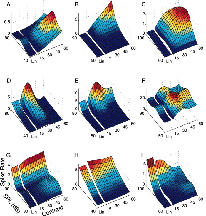
Contrast versus intensity response curves of nine single units. The ripple noise stimulus was presented in pseudorandom order for Lin, 15, 30, 45, and 60 dB and at five intensity conditions (intensity spacing of 10 or 15 dB) for a possible 25 combinations. Surface plots depict the measured spike rate as a function of the stimulus contrast and intensity parameters. Spike rates often increased monotonically with increasing contrast (dynamic range) parameter (A-C) and were typically weakest for the Lin-RN. Other neurons displayed nonmonotonic contrast response curves (D-F) in which the mean spike rate was greatest for contrast values of either 30 or 45 dB. The remaining neurons either had a decreasing monotonic response curve (I) or displayed no statistically significant contrast dependency (G, H).
Figure 4.
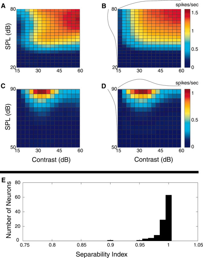
Separability of the contrast-intensity response function. Representative contrast-intensity response curves of a contrast-monotonic (A) and nonmonotonic (C) single neuron. Separable approximations (B, D) closely match the true response curves of A and C. In both cases high separability index values are obtained (0.98 for B and 0.99 for D). The separable response components for contrast and SPL are depicted above and to the left of the separable response curves of B and D. Histogram showing the separability index of n = 63 single units and n = 40 multi-units (E). All neurons had a very high separability index, indicating that the response rate can be expressed as an independent function of contrast and intensity.
We characterized the contrast-response curves of each neuron along the maximum SPL contour according to the shape of the contrast-response curve as increasing-monotonic, nonmonotonic, decreasing-monotonic, or independent of contrast. As a criterion, we searched for statistically significant changes (increase or decrease) in firing rate at each contrast condition. Estimates of the firing rate measurements,
 , over a 60 sec time window were bootstrapped for each contrast condition, M = 15, 30, 45, or 60 dB, to determine the variability of the data. The significance probability was determined numerically for p < 0.05 by finding the tail probabilities of the overlapping firing rate distributions across different contrast conditions. Neurons were identified as contrast nonmonotonic whenever the measured firing rates for the 15 and 60 dB conditions were statistically smaller than for 30 or 45 dB contrast. Mean firing rates for monotonic neurons were chosen to satisfy a significance relationship
 or
or
 .
.
A nonrepeating 18 min segment of the RN was presented at key locations of the contrast-intensity response curve: Lin and 30 dB conditions, Lin and 60 dB conditions, or Lin, 30, and 60 dB conditions. This was used to estimate the STRF of each neuron at multiple-contrast operating conditions. Finally, at 25 recording sites, the mutual information rate of each neuron was estimated from the response rastergrams to a 5 sec segment (repeated 150 times) of the ripple noise (see Mutual information; see Fig. 8).
Figure 8.

Spiking pattern and response reproducibility as a function of contrast for two single neurons. A 5 sec segment of the Lin, 30 dB, and/or 60 dB ripple noise was presented. Rastergrams and PSTHs show 125 response traces to the ripple noise: Lin, 30 and 60 dB for neuron 1 (A, shown top to bottom, respectively) and for neuron 2 (B, shown top to bottom, respectively). Each spike is shown as a single dot (bin width, 1 msec). The PSTH for each condition is shown above the corresponding rastergrams (shown on identical amplitude scales for Lin, 30 dB, and 60 dB). Driven firing rates and response reproducibility improve for the 30 and 60 dB RN relative to Lin-RN. Higher peak-to-trough amplitude modulations of the driven spike rate for 30 and 60 dB indicate that stimulus encoding is improved for the Log condition.
Spectrotemporal receptive field. Contralateral and ipsilateral STRFs are computed by averaging the pre-event spectrotemporal envelope of the contra- and ipsi-stimulus at the time instant of each neural spike, tn (47 μsec resolution):
 |
9 |
Here T corresponds to the experimental recording time in seconds, τ is the temporal delay of the stimulus relative to the neural event time (0-100 msec), S̄(t,Xk) is the zero-mean spectrotemporal envelope for the contra- or ipsi-stimulus, and σs2 is the envelope variance.
All of the analysis was performed so that the spectrotemporal enveloped used in Equation 9 corresponds precisely with the stimulus dimension under consideration. For instance, if the Lin-RN sound was presented (Eq. 8), the linear-amplitude zero-mean spectrotemporal envelope:
 |
10 |
was used to compute the STRF of the neuron where σ2 = β/12 (β = 1 - 10-30/20) is the variance of the envelope and S̄g is the zero-mean, unit-variance generic spectrotemporal RN envelope. Alternately, if a logarithmic-distributed RN envelope was used, e.g., M = 30 dB, the corresponding zero-mean decibel envelope was used in the analysis:
 |
11 |
where σ2 = M2/12 dB2 is the signal variance for the Log sound. This procedure assured that in both instances the stimulus spectrotemporal envelopes used for the reverse correlation were identical in all respects except their variance. Unfortunately, this meant that the STRF units were distinctly different for the Lin- and Log-spectrotemporal envelopes (Eqs. 10 and 11, respectively). These are given as output/input where the output units are spikes per second for either case but the input units are dB for the Log envelope and unitless for the Lin-envelope. Therefore, an alternate normalization was preferred for the STRF in which we removed the input stimulus dimensions by multiplying by the average input signal: STRFr = σ · STRF. This rate-normalized STRF is given in units of spikes per second and corresponds to the average output produced for the average input (Escabí and Schreiner, 2002). Furthermore, after normalizing Equation 9 in this manner, both rate-normalized STRFs are no longer confounded by any stimulus-dependent aspects and are now described by the same equation:
 |
12 |
Throughout this report, the rate-normalized STRF is used to facilitate comparisons.
Statistically significant STRF. Statistically significant regions of the STRF were determined by considering a null condition in which N randomly chosen Poisson spikes are put through Equation 9 (Escabí and Schreiner, 2002). The amplitude distribution of this control-STRF was derived in closed form, and significance was tested for all STRFs at p < 0.002. Because the amplitude distribution of the control-STRF quickly approached a Gaussian distribution (for as few as N = 50 spikes), the significant STRF was obtained by keeping all values that exceeded 3.09 SDs of the control noise STRF and setting all other values to zero (e.g., actual significance p < 0.0019 for N = 50).
STRF similarity index. We compared STRF shapes across multiple conditions with the STRF correlation coefficient or similarity index (SI) (DeAngelis et al., 1999; Reich et al., 2000). For two experiment conditions A and B, we consider the statistically significant vectorized RFs, which consist of all pixels of STRFA and STRFB (determined for both the contra- and ipsi-STRFs) that exceed a significance test (p < 0.002) for condition A or B. The STRF similarity index is then computed as:
 |
13 |
where RFA and RFB are the significant vectorized binaural-STRFs for condition A and B, respectively,
 corresponds to the vector inner product, and ∥·∥ designates the vector norm operator. The SI quantifies the STRF shape differences or similarity independently of STRF amplitude and assumes numerical values between -1 and 1, where 0 designates not similar, 1 indicates that the STRFs have identical shape, and -1 indicates that the STRFs have identical shape but differ by a sign inversion.
Rate and magnitude disparity index. Two metrics were designed that allowed us to evaluate firing rate and STRF energy differences independently of the STRF shape. First we computed a rate disparity index (RDI):
 |
14 |
where λA and λB are the measured firing rates for conditions A and B, respectively, and s = sign (λA - λB). The magnitude of the RDI is numerically equivalent to the percentage of change in firing rate referenced on condition A if s > 0 and B if s < 0. Its sign, s, tells us which condition, A or B, had a higher firing rate: λA > λB if s > 0 and λA < λB if s < 0.
Differences in the driven neuronal activity between two stimulus conditions were quantified by measuring the percentage of change in the STRF energy, which we measured as an STRF magnitude disparity index (MDI):
 |
15 |
where EA and EB are the significant binaural rate-normalized STRF energies for conditions A and B, respectively (Escabí and Schreiner, 2002). The STRF energy measures phase-locked activity (units of spikes per second) that is captured by the STRF of the neuron. Therefore, the MDI measures changes in phase-locked or stimulus-driven neuronal activity where the sign, s, designates which condition was stronger and the magnitude of the MDI designates the percentage of change in driven activity.
Mutual information. A 5 sec segment of the RN stimulus was presented for 150 trials. Response traces were recorded for each trial, and the reliability of the spike train was determined by measuring the mutual information rate (de Ruyter van Steveninck et al., 1997; Strong et al., 1998). The first 25 traces were discarded for all neurons to minimize the effects of adaptation. Each spike trace was digitized at a sampling resolution of Δt = 1 msec, and the spike train entropy was determined by measuring the probability distribution, P(W), of possible N-bit words, W (also tested for Δt = 2 and 5 msec). A search through the whole experiment was conducted to determine the word distribution, P(W). Using the distribution of N-bit words, the spike train entropy is determined as:
 |
16 |
This measure provides a theoretical upper limit on the amount of information that a spike train can convey and does not account for the possibility of internal noise. To determine the noise inherent within the response, the noise entropy was computed by determining the trial-to-trial reliability of the response (e.g., the entropy in the spike train that does not convey any viable information about the stimulus). At any given time instant, t, the conditional probability distribution of obtaining a given N-bit word was computed, P(W|t). The noise entropy was then determined as:
 |
17 |
where
 is the conditional ensemble expectation computed over all time. The information that the spike train contains about the stimulus (i.e., the mutual information) is determined by subtracting these two quantities: I = Stotal - Snoise. This procedure was bootstrapped across different stimulus segments, word lengths (T = 5, 6, 8, 10, 15, 20, 40, 80, 160, and 200 msec), and data fractions (80, 50, 33, and 25%). The mutual information and error bounds were then extrapolated (using 80, 50, 33, and 25% data fractions and T = 5-15 msec) for the infinite data case according to the procedure of Strong et al. (1998). The algorithm was calibrated with fly visual data from Borst (2003).
Spectrotemporal phase-locking index. We measured the contribution of single action potentials by considering how each neuronal spike contributes to the STRF construction procedure (Eq. 12) with a spectrotemporal phase-locking index (PLI) (Escabí and Schreiner, 2002). The PLI metric allows us to measure the degree of alignment of action potentials to the spectrotemporal envelope of the sound and provides a measure of the fraction of the spikes of the neuron that contributes to the STRF construction process.
The theoretical basis for the PLI metric is a tight temporal spike alignment to on- and off-features in the RN sound that will lead to optimal buildup of the STRF (Eq. 12). This will produce a large peak-to-peak STRF amplitude. If the alignment of action potentials and stimulus features is poor, the resulting STRF peak-to-peak amplitude will be small. On the basis of this fact, the phase-locking index is defined as the measured peak-to-peak amplitude of the STRF normalized by the theoretical maximum attainable peak-to-peak amplitude for a perfectly phase-locking neuron:
 |
18 |
where max(STRFr) - min(STRFr) is the measured peak-to-peak amplitude for the rate-normalized STRF (Eq. 12) and √12 · λ is the maximum theoretical value for Equation 12 (Escabí and Schreiner, 2002). The PLI is bounded between 0 for no evident phase locking (no measurable STRF) to 1 for a perfect phase locking.
Results
We studied the amplitude distributions of spectrotemporal modulations in natural sounds to determine whether sensory neurons respond preferentially to sounds with a natural-like dynamic range. First, we quantitatively measured the second-order modulations of various natural sound ensembles. We next tested the representation of linear and logarithmic spectrotemporal modulations to determine whether the amplitude statistics and the dynamic range of the stimulus significantly improve neuronal encoding in the ICC. We designed synthetic RN stimuli that uniformly cover the linear or decibel dimension over a predetermined range of values and are matched to the statistical structure of various artificial stimuli and natural sounds. This approach allowed us to closely match a number of low-order statistics of the linear and log-transform stimulus, such as the SD, modulation depth, and contrast, while allowing us to independently modify the shape of the amplitude distribution and its higher-order moments (e.g., its skewness, kurtosis, and log-transform SD). STRF and information theoretic approaches were then used to compare neuronal encoding abilities for both logarithmic- and linear-ripple noise stimuli and for various dynamic range conditions.
Spectrotemporal modulations and contrast in natural sound
The statistical properties of the spectrotemporal modulations in natural sounds were determined by analyzing an extensive database that included speech, animal vocalizations, environmental sounds, and white noise. Animal vocalizations included sound emissions from a host of domestic (cat, horse, dog, etc.) and nondomesticated (bats, primates, birds, large cats, frogs, etc.) animals. Environmental background sounds were selected from inanimate sources such as running water, wind, and thunder. The sample also included unvocalized sound emissions from animals such as a woodpecker hammering, footsteps in leaves, and buzzing from a swarm of bees. Human speech was conversational, obtained from long, continuous segments of a reproduction of the play Hamlet. All sounds were decomposed into a cochleotopic representation that mimics the output performed by the cochlea (Fig. 1). This spectrotemporal stimulus pattern provides a pictorial representation of the spectral and temporal modulations that are present in each signal.
Figure 1 illustrates representative sound segments from each of the studied stimulus ensembles. The spectrotemporal modulations in each sound are plotted either as a linear amplitude variable (Fig. 1A,E,I,M), normalized to an amplitude range between 0 and 1, or as a log-transform variable expressed in amplitude units of decibels (Fig. 1B,F,J,N). Visually, much of the detail of the linear amplitude spectrotemporal envelope is obscured because most of the stimulus modulations are localized about amplitudes near zero. In contrast, the log-transform spectrotemporal envelope expands the effective dynamic range of each stimulus and expresses the modulations as proportional amplitude, so that much of the structural detail is readily visible. The perceptual difference in the visual representation of these stimuli is consistent with psychophysics of intensity and luminance discrimination, both of which follow Weber's law scaling (Weber, 1834; Fechner, 1860; Miller, 1947; Harris, 1963; Jesteadt and Wier, 1977; Florentine et al., 1987).
We computed the spectrotemporal amplitude distribution of each signal by collapsing all of the pixel values of the spectrotemporal envelopes into a binned histogram. These are shown for both the linear and decibel spectrotemporal envelopes. As observed from the linear spectrotemporal envelopes, the distribution of spectrotemporal amplitudes in natural signals is highly skewed toward values near zero (Fig. 1C,G,K; Table 1). By comparison, white noise has amplitude fluctuations that cover a larger extent of the linear amplitude space (Fig. 1O). Thus, although all natural sounds exhibit spectrotemporal modulations that span nearly the entire range of linear amplitude values (from 0 to 1; all sounds had modulation depths >99.99%), the measured SDs were typically small, indicating that the average amplitude modulations of these signals spanned only a limited region of the linear amplitude space and were skewed toward zero value (Table 1). This conflicting assessment of the spectrotemporal modulations in natural signals indicates that typical measures such as the traditionally defined contrast, C = (SMax - SMin)/(SMax + SMin), or the modulation index, β = (SMax - SMin)/SMax, are inappropriate because they only account for the maximum and minimum stimulus intensities (SMax and SMin, respectively) and do not take into account the distribution of intermediate amplitude values.
The log-transform spectrotemporal envelope histogram expands the observable range of the signal and therefore overcomes many of the limitations observed for the linear amplitude variable. The decibel amplitude modulations in natural sounds follow a roughly symmetric bell-shaped distribution as measured from the low skewness values (Fig. 1D,H,L; Table 1). As is evident in the example spectrotemporal envelopes, the measured SD and 90th percentile range of speech, vocalizations, and environment sounds spanned an extensive range of values (Table 1). Vocalizations and speech have the broadest distributions as measured from their SD and 90th percentile range, whereas environmental sounds covered a narrower range of amplitudes. White noise, by comparison, spanned the narrowest amplitude range.
These findings show that vocalizations and environmental sounds contain logarithmically distributed spectrotemporal modulations with an effective dynamic range (i.e., 90th percentile range; ∼30 dB for environmental sounds and ∼50 dB for vocalizations and speech) that is closely matched to the intensity operating range of neurons in the auditory pathway (Evans and Whitfield, 1964; Palmer and Evans, 1982; Eggermont, 1989). We therefore postulate that auditory neurons use such information for efficiently encoding and detecting spectrotemporal features in natural signals. As is evident from Figure 1, vocalizations and speech dynamically change over time and exhibit short periods of high-energy and low-energy comodulated activity followed by quiet or background activity (Nelken et al., 1999). Background sounds by comparison are usually stationary over the time scales that are relevant for intensity discrimination and loudness perception (Green et al., 1957; Stephens, 1973) and generally have a much narrower dynamic range. These difference in the effective dynamic range and the time-varying structure between vocalization and environmental sounds thus may be important for signal segregation and may facilitate the detection of vocalizations in high levels of background noise.
Contrast and intensity response characteristics
To test the possibility that the operating range of the central auditory system is matched to efficiently process natural acoustic stimuli, we designed naturalistic RN stimuli that mimic the logarithmic amplitude fluctuations observed in natural sounds and a control stimulus with linearly distributed amplitude fluctuations (see Materials and Methods) (Fig. 2) similar to those found in common experimental stimuli. Although the distribution of logarithmic modulations in the log-RN does not exhibit long tails as evident in all natural sounds (Fig. 1), these sounds have spectrotemporal amplitudes that efficiently cover the decibel amplitude space (Fig. 2I,J), an exponential-like linear amplitude distribution (Fig. 2H), and envelope SDs within the range observed for natural sounds (see Materials and Methods) (Tables 1, 2). For both conditions, the modulations in the RN sound covered an unbiased range of temporal (0-350 Hz range) and spectral (0-4 cycles per octave) modulations, making it a suitable test stimulus for measuring spectrotemporal receptive fields in the ICC (Escabí and Schreiner, 2002; Qiu et al., 2003). The spectrotemporal content of all sounds was held fixed, and the amplitude distribution of each sound was varied independently. The naturalistic RN has spectrotemporal intensity fluctuations that uniformly covered a dynamic range of 15, 30, 45, or 60 dB (shown for 45 dB in Fig. 2I,J). The linearly distributed control sound had amplitude fluctuations that uniformly covered a predefined linear amplitude range from 10-30/20 = 0.032 to 1 (modulation index = 0.968) (Fig. 2B,C). Both the naturalistic (Log) and artificial (Lin) stimuli had identical spectrotemporal envelope content and differed only in their amplitude statistics (see Materials and Methods) (Figs. 2A,F).
Recordings were performed on n = 63 su and n = 40 mu in the ICC. Sound segments (15 sec) were presented in a pseudorandom order for the different contrast conditions and for 5 rms sound pressure levels (SPLs) extending over a range of 50 or 75 dB (step size of 10 or 15 dB, respectively). Intensity- versus contrast-response curves were derived for each neuron by measuring the mean spike rate at all operating conditions (see Materials and Methods) (Fig. 3). As expected, neurons showed monotonic or nonmonotonic response characteristics as a function of SPL (Evans and Whitfield, 1964; Ehret and Merzenich, 1988; Eggermont, 1989; Sutter and Schreiner, 1995). Similar dependencies were observed for the contrast axis. Response characteristics can be increasing-monotonic with increasing dynamic range (Fig. 3A-C), tuned (Fig. 3D-F), decreasing-monotonic (Fig. 3I), or independent (Fig. 3G,H) of the stimulus contrast statistics. For reference, results for the Lin stimulus are shown alongside the Log contrast conditions.
Increasing-monotonic units (n = 37 mu + su) showed a significant increase in firing rate (p < 0.05) with increasing contrast dynamic range. In such cases the mean spike rate was typically minimal for the Lin-RN and 15 dB Log-RN and maximal for the 60 dB Log-RN (firing rate increase over Lin: average = 168%, median = 78%). For all neurons, the mean spike rates were similar for linear-RN and 15 dB Log-RN (p > 0.1). Hence, the minor differences between these two stimulus conditions were biologically insignificant. On increasing the dynamic range above 15 dB, spike rates increased monotonically (Fig. 3A: λ15 = 0.10 spikes/sec and λ60 = 0.95 spikes/sec, p < 0.0001; B: λ15 = 0.03 spikes/sec and λ60 = 3.36 spikes/sec, p < 0.0001; C: λ15 = 0.31 spikes/sec and λ60 = 2.15 spikes/sec, p < 0.0001; taken for the intensity with maximum response).
Nonmonotonic contrast response curves were seen in ∼46% of the sites (p < 0.05; n = 47 mu + su) (Fig. 3D-F). Responses were minimal for 15 dB-RN and maximal for Log-RN with a dynamic range of 30 or 45 dB. On increasing the dynamic range to 60 dB, the responses of nonmonotonic neurons were suppressed. On the average, a 34% (multi-unit = 27%) decrease in firing rate was observed for the 60 dB contrast condition (su median = 25%; mu median = 26%; not significantly different, χ2v=5 = 3.75; p = 0.44). The single neuron depicted in Figure 3D has a significant reduction (91%; p < 1 × 10⁻⁶) in firing rate (λ30 = 9.7 spikes/sec and λ60 = 0.9 spikes/sec). Although the observed nonmonotonic relationships were statistically significant, we point out that reductions in firing rate were usually small. The neurons shown in Figure 3, E and F, had a reduction of 49% (λ30 = 14.7 spikes/sec and λ60=7.48 spikes/sec; p < 2 × 10⁻⁶) and 16% (λ30 = 39.0 spikes/sec and λ60 = 33.8 spikes/sec; p < 0.001), respectively. Only four single neurons and three multi-units showed a significant decrease in firing rate to less than half of their maximum response amplitude. Other neurons showed a decreasing trend in firing rates (n = 7) with increasing contrast (Fig. 3I) (λ15 = 2.3 vs λ60 = 0.75 spikes/sec; p < 1 × 10⁻⁶) or showed no statistically significant response pattern (n = 12) (Fig. 3G: λ15 = 3.6 vs λ60 = 4.5 spikes/sec, p > 0.35; H: λ15 = 7.7 vs λ60 = 6.7 spikes/sec, p > 0.4).
Independence of response to intensity and contrast
The contrast-intensity response curves of Figure 3 demonstrate that, in principle, stimulus intensity and contrast can be encoded by the mean firing rate characteristics of individual neurons. The hypothesis that intensity is partly encoded by the mean firing rate of single neurons is consistent with this observation. What is presently not clear is how spectral and temporal fluctuations (which are themselves a form of intensity at very fine spectral and temporal scales) associated with the contrast characteristics of the ripple sound are jointly encoded with intensity by individual or populations of neurons. It is possible that neuronal responses to intensity (SPL) and contrast covary or, alternatively, are processed independently of each other. To determine which of these two possibilities is consistent with the observed data, we determined whether the intensity-contrast rate-level functions are separable for these two parameters.
Intensity-contrast response (for logarithmically distributed RN only) curves were decomposed using a singular value decomposition procedure (Strang, 1988). This procedure decomposes the contrast-intensity response curve into a weighted sum of functions that are each independent products of the contrast (C) and intensity (SPL) parameters. Mathematically the response function can be expressed as:
 |
19 |
where R(C,SPL) is the contrast-intensity response curve, γk is the k-th singular value, and uk(C) and vk(SPL) are functions of contrast and intensity, respectively. If the contrast-intensity response curve is strictly a separable function of SPL and C, it is expected that the above sum degenerates into a single term. For this unique scenario, the response of the neuron is expressed by the first term in the sum R(C,SPL) = γ1 · u1(C) · v1(SPL).
A separable approximation of the contrast-response curve was obtained by considering only the first singular value: R̂(C,SPL) = γ1 · u1(C) · v1(SPL). The separable approximation and the true contrast-intensity response curves are depicted in Figure 4 for two single neurons. In both cases the separable approximation captures most of the detail of the true response function, thus supporting the idea that contrast and intensity are processed independently.
A direct measure of separability is provided by considering the relative strength of the first singular value to the higher-order singular values. Thus we devise a separability index:
 |
20 |
which consists of the ratio of the first singular value,
 , to the weighted sum of all the squared singular values (N = 4 because the measured contrast-intensity response function consists of a 4 × 5 matrix; four contrast versus five intensity conditions). This measure quantifies the overall fraction of the contrast-intensity response curve accounted for by the separable approximation, R̂. Values near zero indicate that the contrast-intensity response curve is strongly nonseparable, whereas values near unity indicate that the response curve is fully separable. The examples of Figure 4 exemplify this point. Both response curves are in close agreement with their separable approximations and consequently the measured separability index values are near unity (Fig. 4A,B: 0.98; C, D: 0.99). Across the population of neurons (n = 63 su and n = 40 mu), the separability index was exceptionally high (Fig. 4E) (mean value = 0.99 ± 0.01; mean ± SD), suggesting that contrast-response characteristics are independent of SPL.
Effects of envelope statistics on spectrotemporal coding
It is conceivable that the auditory system uses the range and shape of the contrast distribution as a secondary acoustic cue. Individual neurons can show nonmonotonic rate response curves to Log-contrast fluctuations that are independent of intensity, reflecting a contrast range sensitivity or even selectivity. For most neurons, the mean response rates were considerably larger for the naturalistic Log-RN than for the control Lin-RN, indicating sensitivity to the shape of the contrast distribution.
Do individual neurons use the dynamic range characteristics in natural sounds to faithfully encode fine spectral and temporal sound components? Can individual neurons more accurately detect specific acoustic features under such naturalistic contrast conditions?
To address these questions, we computed the STRF at different operating points of the contrast-intensity response curve (see Materials and Methods). RN stimuli were presented at identical rms intensity and two or more contrast conditions (Lin vs 30, Lin vs 60, 30 vs 60, or Lin vs 30 vs 60). Figure 5 shows STRFs and the corresponding contrast-intensity response curves for three typical neurons. STRFs were computed at the operating points depicted by the circles on the contrast-intensity response curve (red = Lin, green = 30 dB, and blue = 60 dB). For all conditions, the shape of the STRF is qualitatively similar, indicating that the neuron is responding to similar sound features during all contrast conditions. The mean firing rate and STRF amplitude of the neuron, however, are significantly stronger (p < 0.01) for the Log- than for the Lin-RN stimulus. Comparing the contrast-intensity response curves with the STRF, it is noted that the differential strength of the STRF (units of spikes per second) is increased at contrast operating points where the mean spike rate is likewise increased. This observation indicates that the neuron uses the increased spike rate to encode phase-locked activity with respect to the stimulus spectrotemporal envelope. This response enhancement is typical for the majority of neurons.
Figure 5.

Relationship between the contrast-intensity response curve and the STRF. The contrast-intensity response curve is shown for a contrast nonmonotonic unit (A) and two contrast monotonic neurons (E, I). STRFs were computed at the contrast-intensity operating points designated by the colored circles (red =Lin, green = 30 dB, and blue = 60 dB). B-D show the STRFs for the contrast nonmonotonic neuron depicted in A. Both the mean firing rate and STRF amplitude covary, following a similar nonmonotonic relationship with contrast. The STRF energy for the monotonic neuron depicted in D increases monotonically with increasing contrast (F-H). The neuron of I did not respond to the Lin (J) condition but responded with increased efficacy to the 30 and 60 dB conditions (K, L, respectively). Red contours designate statistically significant regions of the STRF; p < 0.002.
It appears that changing the contrast operating point of the RN input alters the relative amplitude of the STRF and leaves its shape unaffected, suggesting that the neuron responds to similar sound components but with increased or decreased efficacy. To quantify this effect, we measured amplitude and shape differences of the STRF as a function of the contrast and intensity operating point. We considered three metrics that independently quantify STRF shape, amplitude, and firing rate differences. First we computed the STRF similarity index (DeAngelis et al., 1999; Reich et al., 2000; Escabí and Schreiner, 2002). This metric takes values between -1 and +1 and is numerically equivalent to the Pearson correlation coefficient. Next we measured the percentage of change in firing rate and STRF energy with the rate (RDIA,B) and magnitude disparity index (MDIA,B). These metrics quantify changes in firing rate and STRF energy, respectively, between two experiment conditions, A and B, in which the magnitude designates the percentage of change and the sign (+ or -) designates which condition is stronger (A or B, respectively).
Typical neurons depicting differences in STRF shape, firing rate, and STRF energy are shown in Figure 5. The neuron depicted in Figure 5E-H has similar STRFs (SI60,30 = 0.97; SI60,Lin = 0.92; SI30,Lin = 0.91) for all conditions tested. Therefore this neuron responded to identical spectrotemporal sound patterns at all operating points. Despite the similarity in spectrotemporal shape, its RDI and MDI indicate that the neuron responded with a higher spike rate (RDI30,Lin = 390%; RDI60,Lin = 543%) and stronger differential response strengths (MDI30,Lin = 395%; MDI60,Lin = 468%) for the 30 and 60 dB conditions (compared with Lin). Neurons with nonmonotonic contrast dependencies (Fig. 5A-D) typically show higher spike rates for 30 dB Log-RN compared with Lin-RN (RDI30,Lin = 35%); however, their spike rates are typically higher for 30 dB than for 60 dB (RDI60,30 = -43%). The STRF energy of the neuron is likewise greater for the 30 dB contrast than for Lin-RN or 60 dB-RN (MDI30,Lin = 72%; MDI60,Lin = 2.3%; MDI60,30 = -42%). Other neurons (Fig. 5I-K) responded weakly to the Lin-RN and therefore did not produce statistically significant STRFs for this condition. SI values comparing Lin- versus Log-RN for this example were small (SI30,Lin = 0.21 and SI60,Lin = 0.28); however, SI values between the 30 and 60 dB condition were much higher (SI60,30 = 0.88). MDI (MDI30,Lin = 4,558% and MDI60,Lin = 18,120%) and RDI values (RDI30,Lin = 5,589% and RDI60,Lin = 22,130%) were large, suggesting that the neuron responded efficiently to the Log- but not to the Lin-RN.
Similarity index population data are shown in Figure 6 for n = 57 single neurons and n = 75 multi-units. Multi-unit and single unit data showed similar trends and therefore were pooled together for all conditions (30 vs Lin; 60 vs Lin; 60 vs 30). Most neurons had high SI values (mean SI = 0.77; median SI = 0.87) across all conditions, supporting the initial observations (Fig. 5) that most neurons responded to similar spectrotemporal sound features for both Lin- and Log-RN. Other neurons (12 single units and 7 multi-units) had low SI values (SI < 0.5). Inspection of the data revealed that these neurons had statistically significant STRFs (p < 0.002) for the 30 and 60 dB conditions, but not for the Lin-RN because of insufficient number of action potentials (Fig. 5J-L).
Figure 6.

Population similarity index histogram comparing STRF shape across all contrast conditions. Similarity index measurements were obtained by computing the STRF correlation coefficient for the 30 dB versus Lin, 60 dB versus Lin, and 60 dB versus 30 dB contrast conditions (n = 57 single units and n = 75 multi-units). The population histogram is skewed toward +1 (mean = 0.77; median = 0.87), indicating that STRFs for the different contrast conditions have similar spectrotemporal patterns.
RDI and MDI metrics were computed for all single and multi-units to compare the response rate and STRF energy differences for the three contrast conditions (Lin, 30, and 60 dB). The initial observation for the single units of Figure 5 supports the hypothesis that ICC neurons respond more efficiently to decibel fluctuations. Population data further support this possibility. The MDI and RDI metrics were positively skewed and had only a few negative values as indicated in the summary plots of Figure 7. On average, a significant increase in firing rates (mean: RDI30,Lin = 267%, RDI60,Lin = 995%; median: RDI30,Lin = 60%, RDI60,Lin = 172%; t test, p < 0.01) and STRF energy (mean: MDI30,Lin = 135%, MDI60,Lin = 352%; median: MDI30,Lin = 103%, MDI60,Lin = 141%; t test, p < 0.01) was observed for the 30 or 60 dB contrast relative to the Lin-contrast condition. Furthermore, both the MDI and RDI are significantly correlated (r60,Lin = 0.95 ± 0.05; r30,Lin = 0.96 ± 0.04; r60,30 = 0.99 ± 0.01; mean ± SE), indicating that increases in firing rate are accompanied by an STRF strength increase. Because the additional spikes for the 60 and 30 dB conditions (compared with the Lin) must be time locked to the stimulus to produce a difference rate increase in the STRF, this observation indicates that additional spikes for the Log-RN are used directly to encode spectrotemporal information.
Figure 7.

Population response rate and STRF energy statistics comparing Log- and Lin-contrast. RDI and MDI measurements quantify the percentage of increase in firing rate and STRF energy, respectively, for 30 (A) or 60 dB RN (B) relative to the Lin-RN and for 60 dB relative to 30 dB (C). Positive percentage increases indicates higher firing rates or STRF energy, respectively, for 30 and 60 dB conditions compared with Lin (A, B) or for the 60 dB condition relative to 30 dB (C). Negative percentage values indicate that the Lin condition is stronger for the Log versus Lin comparisons (A, B) or that the 30 dB condition was stronger for the 60 dB versus 30 dB comparison (C). RDI and MDI population scatter plots show a large percentage increase in the mean firing rate and the STRF strength for the 30 dB (A) and 60 dB (B) contrast condition relative to Lin. Firing rate and STRF energy increases of >100% were observed for 29 of 53 neurons for 30 dB and 34 of 50 for 60 dB. Seven neurons had MDI and RDI that exceeded 1000% for the 60 dB condition (data not shown). A smaller increase in firing rate and STRF energy is observed for the 60 dB dynamic range compared with 30 dB (C). Both RDI and MDI are significantly correlated (r60,Lin = 0.95 ± 0.05; r30,Lin = 0.96 ± 0.04; r60,30 = 0.99 ± 0.01; mean ± SE). Open circles and triangles represent multi-unit and single-unit data, respectively.
Spectrotemporal phase locking and mutual information
The combined increase in mean firing rate and STRF strength for the decibel contrast conditions indicates that ICC neurons have additional spikes available to encode spectrotemporal information. The observation that STRFs have similar shapes for the Lin- and Log-RN conditions combined with the fact the Lin- and Log-RN sounds have identical spectrotemporal content (because they differ only in their amplitude statistics; see Materials and Methods) further suggests that ICC neurons encode information about similar acoustic features for all of the conditions tested. Given that average spike rates and STRF strengths are higher for the decibel contrast, it is expected that the overall information content conveyed by each neuron is higher for this condition.
The spiking patterns of ICC neurons to the ripple noise stimulus are characterized by phasic response components as depicted in Figure 8. The response rasters and peristimulus time histograms (PSTHs) show a precisely time-locked signature down to a few milliseconds resolution. Inspection of the response rasters and PSTHs for the linear and decibel contrast reveals systematic changes in firing rate and spiking pattern. The increase in firing rate observed for the decibel contrast relative to the linear contrast (mean firing rates) (Fig. 8A: RateLin = 6.3 spikes/sec, Rate30 = 8.5, Rate60 = 11.9 spikes/sec; B: RateLin = 4.4 spikes/sec, Rate30 = 4.2 spikes/sec; Rate60 = 9.0 spikes/sec) was also accompanied by an increase in peak-to-trough amplitude of the phasic response components.
We quantified this effect by measuring the mutual information rate for the Lin, 30 dB, and 60 dB contrast conditions (de Ruyter van Steveninck et al., 1997; Strong et al., 1998). The systematic increases in the observed firing rates are reflected directly in the measured mutual information rate (Fig. 8A: Lin = 24.3 ± 1.2 bits/sec, 30 dB = 39.9 ± 0.5 bits/sec, 60 dB = 56.1 ± 0.9 bits/sec; B: Lin = 10.2 ± 0.9 bits/sec, 30 dB = 11.7 ± 0.7 bits/sec, 60 dB = 22.2 ± 0.9 bits/sec; mean ± SE). Thus each of the example neurons conveys more stimulus-related information for the logarithmic modulation ripple noise. Combined with the fact that the STRF magnitudes are greater for the Log-RN, this finding suggests that the added information carried by the spike train is used directly for more efficient spectrotemporal coding.
Scatter plots and histograms comparing differences in the transmitted information between Log- and Lin-RN are shown in Figure 9, A and B (30 dB vs Lin: 7 su and 7 mu; 60 vs Lin: 7 su and 8 mu). Across the population of neurons there is significant increase in the mutual information rate (Fig. 9B) (47.2 ± 4.2% increase, mean ± SE; 49.6%, median; t test, p < 10-6) for Log- over Lin-RN, although there was no specific enhancement between the 60 and 30 dB ripple noise (30 dB vs Lin = 43.0 ± 3.3% increase; 60 dB vs Lin = 50.0 ± 7.1% increase; paired t test, p > 0.37). This improvement for Log modulations was not accompanied by an equivalent increase in the mutual information per spike (percentage of difference Lin vs Log = 0.50 ± 4.2%; mean ± SE; paired t test, p > 0.8). Thus the increase in the mutual information rate was caused strictly by higher spike rates and not increased spiking precision.
Figure 9.

Mutual information and phase-locking statistics. A, Mutual information rate comparison for the linear and logarithmic ripple noise (30 dB vs Lin, open circles; 60 dB vs Lin, open triangles) shows a net increase in the transmitted information for the Log condition of ∼47.2 ± 4.2% (B). The precise timing of action potentials relative to the sound waveform was quantitatively measured with a phase-locking index (see Materials and Methods). Comparisons for 30 dB (C) and 60 dB (D) relative to the Lin condition show no improvements in the relative timing of action potentials across the tested conditions.
We confirmed this finding by computing a phase-locking index (Escabí and Schreiner, 2002) for each of the measured STRFs (Fig. 9C,D). This metric provides a basis for comparing the precise timing of action potentials on a spike-normalized basis relative to the modulations in the ripple noise sound. A PLI of 0 indicates that the temporal alignment between action potentials and specific instances of the RN sound waveform were poor, whereas a PLI of 1 indicates that the action potentials and the sound waveforms were highly aligned (observed range, 0.014-0.78). The PLI was not statistically different between the linear (0.18 ± 0.01; mean ± SE) and decibel conditions (30 dB = 0.17 ± 0.01; 60 dB = 0.17 ± 0.01; mean ± SE; paired t test: 30 dB vs Lin, p > 0.41; 60 vs Lin, p > 0.77), therefore suggesting that the added information was not caused by improvements of the precise timing of the spike (Fig. 9C,D). These findings therefore reflect a preference for logarithmic over linear modulations that manifests as an increase in the number of evoked action potentials, and not in temporal precision, that collectively contribute to the spectrotemporal coding capacity.
Discussion
This study provides evidence that auditory midbrain neurons use their large intensity operating range for efficiently encoding spectrotemporal information in natural sounds. We find that neural responses are strongly modulated by higher-order amplitude statistics of the spectrotemporal waveform. These changes manifest as increased firing rates, STRF energy, and improved information transmission for decibel modulations compared with linear modulations. Analysis of the receptive field structure further reveals that RF shape is unaffected for all conditions tested. Together these findings indicate that neurons respond to identical spectrotemporal features but with increased efficacy for log modulations. Given that all sensory systems have operating ranges that span several orders of magnitude, and both acoustic and visual stimuli have log-distributed spectral (spatial) and temporal gradations of similar dynamic range (Ruderman and Bialek, 1994; Attias and Schreiner, 1998), our findings support the hypothesis that the large operating range of sensory systems is used for efficient spectrotemporal (spatiotemporal) coding in addition to loudness (luminance) coding.
The structure of natural sounds
The analysis of second-order statistical properties of the spectrotemporal sound representation demonstrates that natural sounds and speech contain spectrotemporal modulations that cover several orders of magnitude, exhibiting nearly symmetric Gaussian-like distribution of log amplitudes. By comparison, the linear amplitude spectrotemporal modulations in natural sounds exhibit sparse segments of high-energy activity, and consequently the linear amplitude distribution of all natural sounds is heavily weighted toward low amplitude values. These results are in contrast to the white noise control, which has spectrotemporal modulations that efficiently cover the linear amplitude dimension.
The range of amplitudes as estimated from the log amplitude SD is greatest for human speech, followed by animal vocalizations and background sounds (Table 1). This extended dynamic range combined with the large amount of temporally comodulated onsets and offsets (Nelken et al., 1999) in communication signals may be necessary to facilitate detection of spectrotemporal features among background signals with highly overlapped spectrotemporal amplitude distributions.
The effective dynamic range of natural sounds represents a salient parameter that could potentially be used by the auditory system to efficiently extract and represent spectrotemporal information. The 90th percentile range of log amplitudes spanned by both environmental sounds (30 dB range) and communication sounds (speech = 49 dB; vocalizations = 43 dB) is comparable with the operating range of peripheral and central auditory neurons for pure tones (Evans and Whitfield, 1964; Palmer and Evans, 1982; Eggermont, 1989). White noise, by comparison, spanned the narrowest range of spectrotemporal amplitudes (18 dB). These results support the idea that the operating range of sensory neurons coevolved with the statistics of natural sensory signals.
Contrast parameters affecting neural responses
We tested whether log-transform amplitude distributions yield a better representation of the sensory signal than linear amplitude by matching various aspects of our RN sounds to the spectrotemporal amplitude distributions of natural sounds and by comparing the response efficiency of neurons. We limited the maximum and minimum excursions in the RN sounds to uniformly cover either the linear amplitude dimension at a fixed modulation depth (97%) or the logarithmic amplitude dimensions for various dynamic range conditions (15-60 dB). The use of uniformly distributed amplitudes for the Log stimulus prevents potentially ambiguous firing rate dependencies that could arise because of the long tails of the amplitude distribution in natural sounds, which could activate intensity-dependent nonlinearities, thereby enhancing or suppressing neuronal activity (Evans and Palmer, 1980; Palmer and Evans, 1980; Ehret and Merzenich, 1988;Eggermont, 1989; Schreiner et al., 1992). This stimulus regimen therefore isolates intensity-dependent effects from purely contrast-dependent mechanisms. We varied the width of the amplitude distribution of the Log-RN sound to address how the dynamic range affects neuronal responsiveness. Finally, the spectrotemporal structure of the RN stimuli is ideal for this analysis because, unlike for natural sounds, it does not contain time-dependent correlations that could potentially engage highly nonlinear response mechanisms (Theunissen et al., 2000; Escabí and Schreiner, 2002).
Firing rates and STRF energies were substantially higher for Log spectrotemporal modulations than for the matched Lin modulations, despite the fact that the 30 dB and Lin sounds were matched in a number of low-order parameters (Table 2) and had nearly identical modulation spectrum (∼2% average difference). In addition, increasing the dynamic range of the Log-RN sound typically increases the neuronal firing rates and receptive field energies, although some neurons also exhibit nonmonotonic dependencies, analogous to neuronal sensitivities for broadband noise in the primary auditory cortex (Barbour and Wang, 2003). Contrast and intensity coding appear to be independent of each other for the tested time scales, supporting the idea that these two stimulus parameters reflect separate neural mechanisms (Fig. 4). Because our analysis represents an intensity-adapted state, it is possible that time-varying intensity changes at a faster time scale, such as for comodulated signals (Nelken et al., 1999), could invoke interactions between intensity and contrast encoding.
How do the observed changes in neuronal firing rate and receptive field energy affect the capacity to encode spectrotemporal information? In nearly all of our neurons, significant changes in the firing rates produced similar changes in receptive field energy (Fig. 7), although the receptive field shape remained constant (Fig. 6). Thus, although the driven activity can change substantially between the different stimulus conditions, neurons appear to respond to very similar sound features. Estimates of the mutual information from the response rastergrams show an average mutual information rate increase of ∼50% for the Log over Lin condition (Fig. 9A,B); however, there is no direct improvement in spike-timing precision as reflected in the phase-locking index and spike-normalized mutual information (Fig. 9C,D). Consequently, neuronal improvements in spectrotemporal encoding ability are caused strictly by increases in the firing rate for the Log-RN condition.
There are two possible ways that higher spike rates improve the overall encoding of spectrotemporal signal components. On the one hand, increasing the spike rate could increase the trial-to-trial reliability of spiking to specific features of the RN stimulus. On the other hand, increases in firing rate could manifest in multiple spikes per feature representation, in which a collection of action potentials collectively encode for a given sound component. Although either one of these mechanisms is consistent with the observed improvements in encoding ability, our preliminary findings support the trial-to-trial reproducibility alternative as the dominant mechanism. This is evidence in the neurons of Figure 8, where the response rasters remain constant but their overall reproducibility improves significantly with increasing spike rate. Thus, for the Log-RN sound, neurons would be able to reliably detect stimulus components that could not be detected for the Lin-RN condition (Fig. 8).
Which specific stimulus parameters contribute to the observed improvements in the spectrotemporal coding ability of inferior colliculus neurons? It is possible that the observed response enhancement to Log-RN conditions arose from trivial low-order stimulus parameters (such as the modulation depth or the maximum intensity) that covary as a function of the performed contrast alterations. To control for this, a number pertinent stimulus statistics were closely considered (Table 2).
The simplest parameter affecting neural responses is the modulation index or contrast. In previous studies, modulation depths were typically varied over a large range (∼5-100%), and these typically elicited increased spike rates and improved phase locking with increasing modulation depths (Rees and Moller, 1983; Krishna and Semple, 2000). The modulation depths in this study varied between 82.2% for the 15 dB-RN and 99.9% for the 60 dB-RN, i.e., the peak-to-trough ratios of the stimulus envelopes were nearly maximal in all instances. Given that output firing rates of many ICC neurons saturate with as little as 20-40% modulation depths and neurons often show modulation gain enhancement (Rees and Moller, 1983; Krishna and Semple, 2000), it is unlikely that the observed effects were directly related to the maximum and minimum amplitude values of the stimulus waveform. To eliminate this possibility, the Lin-RN modulation index was identical to the 30 dB Log-RN (β = 1 - 10-30/20 = 0.968). Despite this match, many neurons showed significantly stronger responses for the 30 dB Log-RN condition.
Other stimulus properties that could affect the comparison between linear and logarithmic stimuli are the waveform linear amplitude SD and the peak intensity offset. Stimulus differences for these properties were either not systematically expressed across all of the stimulus conditions or were too small to account for the large systematic differences in neuronal activity. For the contrast-matched 30 dB Log-RN and Lin-RN conditions, the 30 dB Log-RN has a slightly smaller linear amplitude SD (σLin = 0.280 vs σ30 = 0.257; 8% difference), which is inconsistent with the large increase in firing rates and STRF energies. Although all sounds were matched for their average (RMS) intensity, the peak intensities were different for each sound (Table 2). This subtle but undesirable effect is a direct consequence of the varying degrees of skewness in the spectrotemporal envelope waveforms; however, the peak intensity differences between the Log and Lin (0.75 dB for 30 dB vs Lin; 1.9 dB for 60 dB vs Lin) were typically too small to account for the large increases in neural firing rates for the Log-ripple noise.
The most likely parameters accounting for the observed changes in the neuronal responses are the spectrotemporal envelope skewness and the log-amplitude SD. The contrast distribution for the control Lin- and Log-RN differed significantly if computed on the logarithmic or linear amplitude dimensions (Fig. 2). As for natural sounds (Fig. 1), the linear amplitude distribution of the Log-RN has skewed values toward zero. As the dynamic range of the Log-RN sound is increased from 15 to 60 dB, the measured skewness increases accordingly from 0.59 to 1.96. By comparison, the Lin-RN stimulus is perfectly symmetric with a skewness value of zero (Fig. 2C). Similarly, in the log-amplitude dimension, the width of the amplitude distribution (i.e., the SD) of the Log-RN is seen to increase systematically with increasing dynamic range. Given that response efficacy increased on the average with increasing log dynamic range or with increasing skewness, it is likely that these parameters account for the observed response enhancement in the Log conditions.
Functional implications for spectrotemporal sound analysis
Studies of pure tone transients and onsets in the auditory nerve and auditory cortex have demonstrated that first-spike latency and response amplitude are strongly affected by the onset waveform on the peripheral integration mechanism (Heil, 1997a,b; Heil and Irvine, 1997; Heil and Neubauer, 2001). In particular, the time to first-spike latency is inversely proportional to the peak acceleration or velocity of the sound pressure envelope.
One possible explanation for our findings on information transmission and spectrotemporal coding is that the spectral and temporal acceleration and velocity profiles of the RN envelope account for observed response improvement. The increased mean firing rates for Log-RN indicate that additional spikes are used to encode spectrotemporal information, consistent with the observed increase in the peak-to-trough amplitude of responses as a function of dynamic range (Fig. 8). Unlike the results of onset transients (Heil, 1997a,b), however, we find no analogous improvement in the precision of spike timing. Our results on phase locking suggest that on a spike-normalized basis, the precision of action potentials is constant for the Log and Lin conditions. Given that STRF shapes are identical at all contrast conditions, these observations demonstrate that sounds with logarithmic modulations improve the reliability and throughput of individual neurons, allowing them to faithfully encode those stimulus features that resemble the STRF of the neuron.
This net improvement in firing rates can be explained partly by the fact that Log-amplitude fluctuations in the RN have varying degrees of skewness. Because the skewness of the RN envelope is directly proportional to the spectral and temporal acceleration and velocity of the spectrotemporal envelope of the sound (Fig. 10), our findings are consistent with previously reported findings with onset transients. The range of spectrotemporal velocities-accelerations for the RN sounds is greater for the 30 dB than for the Lin condition and increases proportionally to the dynamic range of the Log-RN (Fig. 10). This difference can activate similar mechanisms as invoked by narrowband onsets (Heil and Neubauer, 2001), thereby increasing spike rates and STRF energies by improving the reliability of spike generation.
Figure 10.

Temporal velocity profile and velocity statistics. A, A temporal cross section of the Lin (continuous), 30 dB (dashed-dot), and 60 dB (dotted) ripple noise (Fig. 2) expressed as a linear amplitude variable, s(t). B, The temporal velocity profile of s(t) is obtained by differentiating each of the respective temporal waveforms. C, The distribution of linear amplitudes (shown for amplitudes from 0 to 0.5) and the distribution of temporal velocities (D). The amplitude distribution for the Lin sound is symmetrically distributed. The 30 and 60 dB RN follow an exponential-like distribution where the skewness is highest for the 60 dB case. The observed range and SD of temporal velocities (D) for each stimulus becomes expanded with increasing skewness of s(t).
Other related mechanisms observed for sinusoidal AM likely play a role as well. These include nonlinear contrast normalization that appears to be expansive for low modulation depths and saturating for large modulation depths (Krishna and Semple, 2000). Enhancement and suppression in the response area of the neuron as a function of SPL, modulation depth, and modulation frequency (Krishna and Semple, 2000) can also fine tune neuronal selectivity, thereby increasing specificity of the neural output. The fact that neurons produce similar STRFs for Log-RN (mean SI = 0.77), but with increased spike rates and STRF energies, suggests that the additional spikes encode for acoustic features with similar spectrotemporal content that were not detected during the Lin-RN. Such a mechanisms could benefit natural sound processing by improving detectability of weak signals in noise and guaranteeing that both large and small amplitude fluctuations are encoded adequately. This is especially important for encoding spectrotemporal modulations natural vocalization signals (Fig. 1A-H) because these can cover several orders of magnitude in their instantaneous spectrotemporal intensities and are often superimposed on background noise with similar statistical properties (Fig. 1I-L).
Although temporal integration certainly plays an important role in the shaping of neuronal sensitivities to our Log- and Lin-RN stimuli (Attias and Schreiner, 1998), our results cannot rule out the possibility that spectral integration mechanisms also contribute to the observed differences between the Log- and Lin-RN and the different dynamic range conditions tested. Our data cannot distinguish between the types of spectral and temporal mechanisms involved. Given that auditory cortical responses to broadband sounds become preferentially tuned for large dynamic range (up to 40 dB), this is not an unlikely scenario for the ICC (Calhoun and Schreiner, 1998). Similar to the observed nonmonotonic dependencies with increasing dynamic range (Fig. 3), recent studies have also shown an analogous form of spectral contrast tuning in the primary auditory cortex of primates (Barbour and Wang, 2003). Our data, however, show that the origins of this form of dynamic range tuning are located or at least initiated subcortically, although it may be further enhanced at the cortical level. Taken together, our findings provide evidence that the dynamic range and skewness of natural sound envelopes are a critical cue for spectrotemporal integration and sound processing.
Implications for sensory perception
The hypothesis that the human ear is adapted to encode signals with large dynamic range is supported by human speech studies. Analyses of the spectral envelopes of speech have shown that the peak-to-valley ratios in human speech (vowel formants) can extend over >20 dB (Plomp, 1983). Spectral peaks associated with vowel formants provide a critical cue for the perception of vowel sounds. Given the large amount of across-subject variability inherent in natural speech, human perception must be robust to envelope alterations under many operating conditions. Production of same vowels by different speakers, for examples, shows a large amount of inter-subject variability with an average intensity SD near 16 dB (Pols et al., 1969; Klein and Plomp, 1970). Additional sources of envelope noise (∼5 dB) are introduced by the reverberant characteristics associated with environmental and room acoustics (Schroeder et al., 1974), yet psychoacoustic studies indicate that perception of vowel sounds is tolerant to such alterations. For example, the just noticeable peak-to-valley ratio of vowel envelopes can be exceptionally large (Ghitza and Goldstein, 1983) and is relatively robust to noise contamination. Such contrast-related cues likely play a critical role in speech perception because increasing the decibel contrast alters the perceived sound in such a manner that it improves intercategory discrimination of vowel sounds (van-Veen and Houtgast, 1985).
A critical question raised by these findings is whether the nervous system processes linear amplitude or decibel amplitude gradations. Historically temporal modulation signals (both in auditory and visual modalities) have been defined on a linear amplitude dimension essentially because of convenience and because these conform to the mathematical conventions devised for communications engineering that came about during the advent of radio and telephony (Hilbert, 1912). In general there is no a priori reason for using linear or decibel amplitude fluctuations as the pertinent stimulus parameter. Thus, the choice of assigning the linear amplitude as the relevant stimulus variable has been arbitrary, for the most part. Only through proper examination can one determine which of these dimensions is most suitable for defining and quantifying the response characteristics of a sensory system.
Studies on loudness coding and intensity discrimination support the notion that decibel amplitude is the more relevant stimulus variable. Human perception of loudness follows linear relationship with sound pressure level (measured in decibels) over most of the hearing range (Stevens, 1957, 1972). Intensity discrimination thresholds are constant (∼0.5 dB) throughout most of the hearing range following the well known Weber's law(Weber, 1834; Fechner, 1860; Miller, 1947; Harris, 1963; Jesteadt and Wier, 1977; Florentine et al., 1987). The fact that response level curves of neuronal data also follow a simple monotonically increasing function of decibel intensity further supports the hypothesis that decibel amplitudes are most suitable for describing physiologic data (Evans and Palmer, 1980; Palmer and Evans, 1980; Ehret and Merzenich, 1988; Eggermont, 1989; Schreiner et al., 1992). Because the spectrotemporal envelope is simply an extension of the intensity variable that extends over time and along the sensory epithelium receptor surface, it is not surprising that the auditory system processes spectrotemporal information in a similar manner as it would for intensity. Our finding that spectrotemporal fluctuations of natural sounds extend over a comparable range of differential intensities as the operating range of single auditory neurons (Evans and Palmer, 1980; Viemeister, 1988) suggests that the operating range of auditory neurons is matched to the dynamic range of natural sounds. Aside from the well accepted doctrine that sensory systems use their large operating range directly for level coding, our findings suggest that it is also used for efficiently processing spectrotemporal information in natural acoustic stimuli with a comparable dynamic range.
Footnotes
This work was supported by National Institutes of Health Grants DC02260 (C.E.S.) and HD20806 (H.L.R., M.A.E.) and a grant from the University of Connecticut Research Foundation (M.A.E.). We thank two anonymous reviewers for numerous comments and suggestions.
Correspondence should be addressed to Monty A. Escabí, University of Connecticut, Electrical and Computer Engineering, 371 Fairfield Road U-1157, Storrs, Connecticut 06269-1157. E-mail: escabi@engr.uconn.edu.
Copyright © 2003 Society for Neuroscience 0270-6474/03/2311489-16$15.00/0
References
- Akeroyd MA, Patterson RD ( 1997) A comparison of detection and discrimination of temporal asymmetry in amplitude modulation. J Acoust Soc Am 101: 430-439. [DOI] [PubMed] [Google Scholar]
- Attias H, Schreiner CE ( 1997) Temporal low-order statistics of natural sounds. In: Advances in neural information processing systems 9 (Mozer MC, Jordan MI, Petsche T, eds), pp 27-33. Cambridge, MA: MIT. [Google Scholar]
- Attias H, Schreiner CE ( 1998) Coding of naturalistic stimuli by auditory midbrain neurons. In: Advances in neural information processing systems 10 (Jordan MI, Kearns MJ, Solla SA, eds), pp 103-109. Cambridge, MA: MIT. [Google Scholar]
- Barbour DL, Wang X ( 2003) Contrast tuning in auditory cortex. Science 299: 1073-1075. [DOI] [PMC free article] [PubMed] [Google Scholar]
- Barlow H ( 1953) Summation and inhibition in the frog retina. J Physiol (Lond) 119: 69-78. [DOI] [PMC free article] [PubMed] [Google Scholar]
- Barlow H ( 1961) The coding of the sensory message. In: Current problems in animal behavior (Thorpe WH, Zangwill OL, eds), pp 217-234. Cambridge, MA: MIT.
- Borst A ( 2003) Noise, not stimulus entropy, determines neural information rate. J Comp Neurosci 14: 23-31. [DOI] [PubMed] [Google Scholar]
- Calhoun BM, Schreiner CE ( 1998) Spectral envelope coding in cat primary auditory cortex: linear and non-linear effects of stimulus characteristics. Eur J Neurosci 10: 926-940. [DOI] [PubMed] [Google Scholar]
- Dan Y, Atick JJ, Reid RC ( 1996) Efficient coding of natural scenes in the lateral geniculate nucleus: experimental test of a computational theory. J Neurosci 16: 3351-3362. [DOI] [PMC free article] [PubMed] [Google Scholar]
- DeAngelis GC, Ghose GM, Ohzawa I, Freeman RD ( 1999) Functional micro-organization of primary visual cortex: receptive field analysis of nearby neurons. J Neurosci 19: 4046-4064. [DOI] [PMC free article] [PubMed] [Google Scholar]
- de Ruyter van Steveninck RR, Lewen GD, Strong SP, Koberle R, Bialek W ( 1997) Reproducibility and variability in neural spike trains. Science 275: 1805-1808. [DOI] [PubMed] [Google Scholar]
- Dong DW, Atick JJ ( 1995) Statistics of natural time-varying images. Network 6: 345-358. [Google Scholar]
- Eggermont JJ ( 1989) Coding of free field intensity in the auditory midbrain of the leopard frog. I. Results for tonal stimuli. Hear Res 40: 147-165. [DOI] [PubMed] [Google Scholar]
- Ehret G, Merzenich MM ( 1988) Neuronal discharge rate is unsuitable for encoding sound intensity at the inferior-colliculus level. Hear Res 35: 1-7. [DOI] [PubMed] [Google Scholar]
- Emmons LH, Whitney BM, Ross DL ( 1997) Sounds of neotropical rainforest mammals. Ithaca, NY: The Library of Natural Sounds-Cornell Lab of Ornithology.
- Escabí MA, Schreiner CE ( 2002) Nonlinear spectrotemporal sound analysis by neurons in the auditory midbrain. J Neurosci 22: 4114-4131. [DOI] [PMC free article] [PubMed] [Google Scholar]
- Evans EF, Palmer AR ( 1980) Relationship between the dynamic range of cochlear nerve fibres and their spontaneous activity. Exp Brain Res 40: 115-118. [DOI] [PubMed] [Google Scholar]
- Evans EF, Whitfield IC ( 1964) Classification of unit responses in the auditory cortex of the unanesthetized and unrestrained cat. J Physiol (Lond) 171: 476-493. [DOI] [PMC free article] [PubMed] [Google Scholar]
- Fechner GT ( 1860) Elemente der psychophysik (éléments de méphysique). Leipzig: Breitkopf and Härtel.
- Florentine M, Buss S, Mason CR ( 1987) Level discrimination as a function of level for tones from 0.25-16 kHz. J Acoust Soc Am 81: 1528-1541. [DOI] [PubMed] [Google Scholar]
- Ghitza O, Goldstein JL ( 1983) JNDs for the spectral envelope parameters in natural speech. In: Hearing: physiological bases and psychophysics (Klinke R, Hartmann R, eds), pp 353-359. New York: Springer.
- Green DM, Birdshall TG, Tanner WP ( 1957) Signal detection as a function of signal intensity and duration. J Acoust Soc Am 29: 523-531. [Google Scholar]
- Greenwood DD ( 1990) A cochlear frequency-position function for several species-29 years later. J Acoust Soc Am 87: 2592-2605. [DOI] [PubMed] [Google Scholar]
- Harris JD ( 1963) Loudness discrimination. J Speech Hear Disord 11: 1-63. [Google Scholar]
- Heil P ( 1997a) Auditory cortical onset responses revisited. I. First-spike timing. J Neurophysiol 77: 2616-2641. [DOI] [PubMed] [Google Scholar]
- Heil P ( 1997b) Auditory cortical onset responses revisited. II. Response strength. J Neurophysiol 77: 2642-2660. [DOI] [PubMed] [Google Scholar]
- Heil P, Irvine DR ( 1997) First-spike timing of auditory-nerve fibers and comparison with auditory cortex. J Neurophysiol 78: 2438-2454. [DOI] [PubMed] [Google Scholar]
- Heil P, Neubauer H ( 2001) Temporal integration of sound pressure determines thresholds of auditory-nerve fibers. J Neurosci 21: 7404-7415. [DOI] [PMC free article] [PubMed] [Google Scholar]
- Hilbert D ( 1912) Grundzüge einer allgemeinen Theorie der linearen Integralgleichungen. Leipzig: Teubner.
- Irino T, Patterson RD ( 1996) Temporal asymmetry in the auditory system. J Acoust Soc Am 99: 2316-2331. [DOI] [PubMed] [Google Scholar]
- Jesteadt W, Wier CC ( 1977) Intensity discrimination as a function of frequency and sensation level. J Acoust Soc Am 61: 169-177. [DOI] [PubMed] [Google Scholar]
- Klein W, Plomp R, Pols LCW ( 1970) Vowel spectra, vowel spaces, and vowel identification. J Acoust Soc Am 48: 999-1009. [DOI] [PubMed] [Google Scholar]
- Krishna BS, Semple MN ( 2000) Auditory temporal processing: responses to sinusoidally amplitude-modulated tones in the inferior colliculus. J Neurophysiol 84: 255-273. [DOI] [PubMed] [Google Scholar]
- Lewicki MS ( 1994) Bayesian modeling and classification of neural signals. Neural Comput 6: 1005-1029. [Google Scholar]
- Lewicki MS ( 2002) Efficient coding of natural sounds. Nat Neurosci 5: 356-363. [DOI] [PubMed] [Google Scholar]
- Lu T, Liang L, Wang X ( 2001) Neural representations of temporally asymmetric stimuli in the auditory cortex of awake primates. J Neurophysiol 85: 2364-2380. [DOI] [PubMed] [Google Scholar]
- Miller GA ( 1947) Sensitivity to changes in the intensity of white noise and its relation to masking and loudness. J Acoust Soc Am 191: 609-619. [Google Scholar]
- Nelken I, Rotman Y, Bar-Yosef O ( 1999) Responses of auditory-cortex neurons to structural features of natural sounds. Nature 397: 154-157. [DOI] [PubMed] [Google Scholar]
- Palmer AR, Evans EF ( 1980) Cochlear fibre rate-intensity functions: no evidence for basilar membrane nonlinearities. Hear Res 2: 319-326. [DOI] [PubMed] [Google Scholar]
- Palmer AR, Evans EF ( 1982) Intensity coding in the auditory periphery of the cat: responses of cochlear nerve and cochlear nucleus neurons to signals in the presence of bandstop masking noise. Hear Res 7: 305-323. [DOI] [PubMed] [Google Scholar]
- Plomp R ( 1983) The role of modulations in hearing. In: Hearing: physiological bases and psychophysics (Klinke R, Hartmann R, eds), pp 270-275. New York: Springer.
- Pols LCW, Kamp LJT, Plomp R ( 1969) Perceptual and physical space of vowel sounds. J Acoust Soc Am 46: 458-467. [DOI] [PubMed] [Google Scholar]
- Qiu A, Schreiner CE, Escabí MA ( 2003) Gabor analysis of auditory midbrain receptive fields: spectrotemporal and binaural composition. J Neurophysiol 90: 456-476. [DOI] [PubMed] [Google Scholar]
- Rees A, Moller AR ( 1983) Responses of neurons in the inferior colliculus of the rat to AM and FM tones. Hear Res 10: 301-330. [DOI] [PubMed] [Google Scholar]
- Reich DS, Mechler F, Purpura KP, Victor JD ( 2000) Interspike intervals, receptive fields, and information encoding in primary visual cortex. J Neurosci 20: 1964-1974. [DOI] [PMC free article] [PubMed] [Google Scholar]
- Rieke F, Bodnar DA ( 1995) Naturalistic stimuli increase the rate and efficiency of information transmission by primary auditory afferents. Proc R Soc Lond B Biol Sci 262: 259-265. [DOI] [PubMed] [Google Scholar]
- Roark RM, Escabí MA ( 1999) B-spline design of maximally flat and prolate spheroidal-type FIR filters. IEEE Trans Signal Process 47: 701-716. [Google Scholar]
- Ruderman DL ( 1997) Origins of scaling in natural images. Vision Res 37: 3385-3398. [DOI] [PubMed] [Google Scholar]
- Ruderman DL, Bialek W ( 1994) Statistics of natural images: scaling in the woods. Phys Rev Lett 73: 814-817. [DOI] [PubMed] [Google Scholar]
- Schreiner CE, Mendelson JR, Sutter ML ( 1992) Functional topography of cat primary auditory cortex: representation of tone intensity. Exp Brain Res 92: 105-122. [DOI] [PubMed] [Google Scholar]
- Schroeder MR, Gottlob D, Siebrasse KF ( 1974) Comparative study of European concert halls: correlation of subjective preferences with geometric and acoustic parameters. J Acoust Soc Am 56: 1195-1201. [Google Scholar]
- Shakespeare W ( 1992) BBC Radio Presents: Hamlet (K. Branagh and G. Dearman). New York: Bantam Doubleday Dell Audio.
- Stanley GB, Li FF, Dan Y ( 1999) Reconstruction of natural scenes from ensemble responses in the lateral geniculate nucleus. J Neurosci 19: 8036-8042. [DOI] [PMC free article] [PubMed] [Google Scholar]
- Stephens SDG ( 1973) Auditory temporal integration as a function of intensity. J Sound Vibration 30: 109-126. [Google Scholar]
- Stevens SS ( 1957) On the psychophysical laws. Psychol Rev 64: 153-181. [DOI] [PubMed] [Google Scholar]
- Stevens SS ( 1972) Perceived level of noise by Marck VII and decibels (E). J Acoust Soc Am 93: 425-434. [Google Scholar]
- Storm J ( 1994a) Great Smokey Mountains National Park: summer and fall. Ithaca, NY: The Library of Natural Sounds-Cornell Lab of Ornithology.
- Storm J ( 1994b) Great Smokey Mountains National Park: winter and spring. Ithaca, NY: The Library of Natural Sounds-Cornell Lab of Ornithology.
- Strang G ( 1988) Linear algebra and its applications. San Diego: Harcourt Brace.
- Strong SP, Koberle R, DeRuyter Van Steveninck RR, Bialek W ( 1998) Entropy and information in neural spike trains. Phys Rev Lett 80: 197-200. [Google Scholar]
- Sutter ML, Schreiner CE ( 1995) Topography of intensity tuning in cat primary auditory cortex: single-neuron versus multiple-neuron recordings. J Neurophysiol 73: 190-204. [DOI] [PubMed] [Google Scholar]
- Theunissen FE, Sen K, Doupe AJ ( 2000) Spectral-temporal receptive fields of nonlinear auditory neurons obtained using natural sounds. J Neurosci 20: 2315-2331. [DOI] [PMC free article] [PubMed] [Google Scholar]
- van-Veen TM, T. Houtgast ( 1985) Spectral sharpness and vowel dissimilarity. J Acoust Soc Am 77: 628-634. [DOI] [PubMed] [Google Scholar]
- Viemeister NF ( 1988) Intensity coding and the dynamic range problem. Hear Res 34: 267-274. [DOI] [PubMed] [Google Scholar]
- Voss RF, Clarke J ( 1975) “1/f noise” in music and speech. Nature 258: 317-318. [Google Scholar]
- Weber EH ( 1834) De pulse, resorptione, auditu et tactu. Leipzig: Koehler.