How Spike Generation Mechanisms Determine the Neuronal Response to Fluctuating Inputs

Abstract

This study examines the ability of neurons to track temporally varying inputs, namely by investigating how the instantaneous firing rate of a neuron is modulated by a noisy input with a small sinusoidal component with frequency (f). Using numerical simulations of conductance-based neurons and analytical calculations of one-variable nonlinear integrate-and-fire neurons, we characterized the dependence of this modulation on f. For sufficiently high noise, the neuron acts as a low-pass filter. The modulation amplitude is approximately constant for frequencies up to a cutoff frequency, f_c, after which it decays. The cutoff frequency increases almost linearly with the firing rate. For higher frequencies, the modulation amplitude decays as C/f^α, where the power α depends on the spike initiation mechanism. For conductance-based models, α = 1, and the prefactor C depends solely on the average firing rate and a spike “slope factor,” which determines the sharpness of the spike initiation. These results are attributable to the fact that near threshold, the sodium activation variable can be approximated by an exponential function. Using this feature, we propose a simplified one-variable model, the “exponential integrate-and-fire neuron,” as an approximation of a conductance-based model. We show that this model reproduces the dynamics of a simple conductance-based model extremely well. Our study shows how an intrinsic neuronal property (the characteristics of fast sodium channels) determines the speed with which neurons can track changes in input.

Introduction

The input-output transformation performed by a neuron is classically characterized by its frequency-current (f-I) relationship (McCormick et al., 1985; Powers and Binder, 2001). However, knowing of this relationship is not enough to predict neuronal responses to transients or time-dependent inputs, a problem that is, in general, particularly tricky because of the highly nonlinear nature of action potential generation. Nevertheless, if the temporal variations of the input are small enough, the dynamics are dominated by the linear response properties of the neuron. Therefore, the response of the neuron to an arbitrary input with weak temporal variations can be predicted if we can determine how its instantaneous firing rate is modulated by sinusoidal inputs.

The response of neurons to sinusoidal inputs has been investigated in various in vitro preparations, including the horseshoe crab Limulus polyphemus (Knight, 1972b), visual cortex (Carandini et al., 1996; Nowak et al., 1997), and vestibular nuclei (Ris et al., 2001; Sekirnjak and du Lac, 2002). Most of these studies restricted their analysis to low-frequency inputs (<20 Hz). Carandini et al. (1996) found that the response of regular-spiking cortical cells to injection of a broadband noisy input is linear and can be flat up to 100 Hz. Bair and Koch (1996), using in vivo recordings in middle temporal (MT) cortex of anesthetized monkeys, showed that the power spectra of the responses of neurons to randomly moving dots are low-pass with a broad range of cutoffs up to 150 Hz.

The linear response of neurons to noisy fluctuating inputs has also been investigated in theoretical studies relying on the leaky integrate-and-fire (LIF) model (Knight, 1972a; Gerstner, 2000; Brunel et al., 2001; Fourcaud and Brunel, 2002; Mazurek and Shadlen, 2002). It was found that in the presence of white noise, LIF neurons behave like low-pass filters, with a cutoff depending on the passive membrane time constant and the average firing rate of the neuron. The gain of the filter decays as 1/√f, where f is the input frequency, and its phase shift reaches the value of 45°, at sufficiently large f. It was also found that temporal correlations in the input noise improve the “accuracy” of the LIF response, because they suppress the decay at high frequencies and reduce the phase shift (Gerstner, 2000; Brunel et al., 2001; Fourcaud and Brunel, 2002). In the present study, we show that simple conductance-based (CB) models behave differently. Using a combined analytical and numerical approach, we investigated theoretically how neuronal properties affect the response of neurons to fluctuating inputs. In particular, we demonstrate that the suppression of the AC part of the spike response to fast varying inputs depends on the DC response of the neuron and on the characteristics of the fast sodium currents responsible for spike initiation.

Materials and Methods

Linear response of the instantaneous firing rate. We investigated the response of a neuron to a time-varying input. Our goal is to determine the instantaneous firing rate ν(t) (i.e., the probability that the neuron will fire between time t and time t ± dt, divided by dt, in the limit dt → 0). We assume that the neuron receives an input

1

where I₀ is the DC component of the input, δI(t) is its deterministic temporal variation around I₀, and I_noise is a noisy component that is described in more detail below. The firing rate ν(t) is determined as a function of I₀ ± δI(t) by averaging the response of the neuron over different realizations of I_noise. Equivalently, ν(t) represents the instantaneous firing rate of a population of noninteracting neurons that receive the same input I₀ + δI(t), but in which each neuron receives an independent realization of the noise.

In the limit of small δI(t), a linear relationship can be written between ν(t) and δI(t):

2

where Φ(I₀) is the average firing rate of the neuron in response to a current I₀ in the presence of noise I_noise (the f-I curve of the neuron), and the kernel, κ, depends on I₀ and the properties of the noise. In particular, the response to a sinusoidally and weakly modulated I_syn(t):

3

where I₁ << I₀ is:

4

where ν₀ = Φ(I₀), and ν₁(f) and ϕ(f) are related to the modulus and the argument of the Fourier transform of κ, , by and .

The gain of the response at frequency f, ν₁(f)/I₁, and the phase response, ϕ(f), completely characterize the linear filtering properties of the neuron. We compute these quantities as a function of the frequency f. Note that at sufficiently low frequencies, it is straightforward to relate the gain ν_LF/I₁ to the f-I curve of the neuron. Indeed, for small f, one can write ν(t) = Φ[I₀ + I₁ cos(2πft)], so that because I₁ << I₀:

5

whereas the phase shift at small f is ϕ_LF = 0.

Noise. When a neuron receives a large number of synaptic inputs per membrane time constant through synapses with small amplitude compared with threshold, the resulting currents can be well approximated by a mean input current with random Gaussian variations around the mean (diffusion approximation) (Tuckwell, 1988); thus, we consider Gaussian noise. If one assumes that postsynaptic currents are instantaneous, the Gaussian noise is white. For exponentially decaying synaptic currents, the Gaussian noise is colored with a correlation time equal to the synaptic decay time constant (see Appendix B2).

Conductance-based models

Two single-compartment neuronal models are used in this study. The first was proposed by Wang and Buzsáki (1996), which is a modified version of the original Hodgkin-Huxley model (Hodgkin and Huxley, 1952). The Wang-Buzsáki (WB) model has a leak current, a fast sodium current with instantaneous activation dynamics, m(V), and a delayed-rectifier potassium current. The firing current threshold of the neuron is I_T = 0.16 μA/cm². This corresponds to a voltage threshold V_T = -59.9 mV. Note that the WB model is type I (zero firing frequency at threshold) and not type II (nonzero firing frequency at threshold), like the Hodgkin-Huxley model with standard parameters (Hodgkin and Huxley, 1952) because of the different choice of parameters, in particular for the sodium and potassium conductance (Wang and Buzsáki, 1996).

The second model was proposed by Hansel and van Vreeswijk (2002), which has the fast sodium current and the delayed rectifier current of the WB model but also additional intrinsic currents: A-type current, slow potassium current, and persistent sodium current. Details of the models are given in Appendix A.

Numerical integration of CB models. Model equations in the presence of noise have been integrated using a stochastic second-order Runge Kutta (RK2) method (Honeycutt, 1992), with a time step <0.02 msec in all simulations. The instantaneous firing rate was computed by taking the average spike count in bins of one-thirtieth of the input period over a minimum of 2000 periods. The obtained instantaneous firing rate was fitted by a sinusoid (Eq. 4) using a least-square method or by computing directly the first Fourier component of the output spike train. Both methods yielded the same results. The input modulation amplitude I₁ was adjusted depending on the input frequency to get an instantaneous firing rate modulation equal to 25% of the baseline. We checked that, to this level of input modulation, the amplitude of the firing rate modulation ν₁ varied linearly with I₁.

Nonlinear integrate-and-fire neuron models

To understand the factors that determine the response to time-varying inputs, we investigated simpler models that are to some extent analytically tractable. We introduced a family of one-variable neuronal models whose membrane potential V dynamics are given by:

6

where C is the membrane capacitance, g_L is the leak conductance, V_L is the leak potential, I_syn is the external synaptic current (Eq. 3), and ψ(V) is a function of voltage that describes the spike-generating currents. The passive membrane time constant is τ_m = C/g_L.

The LIF (Knight, 1972a; Tuckwell, 1988) is the special case of this family of models for which ψ(V) = 0. In this model, a spike threshold V_th has to be imposed to obtain spike generation. The resulting spike is instantaneous, and the neuron is reset to a voltage V_r after a spike.

When the function ψ(V) is supralinear, the membrane potential diverges to infinity in finite time if the input current exceeds some threshold. This divergence can be identified with the firing of a spike, provided that one supplements Equation 6 with a reset condition for the membrane potential to a value V_r, as in the LIF model. A threshold voltage V_T can be defined as the voltage at which the slope of the I-V curve vanishes, which is given by:

7

This is also the largest steady voltage at which the neuron can be maintained by a constant input current. The corresponding current I_T = g_L(V_T - V_L) - ψ(V_T) is the threshold current above which tonic firing occurs. We also defined the spike slope factor Δ_T (in mV) as:

8

This parameter, which is inversely proportional to the curvature of the I-V curve at the threshold V_T, measures the sharpness of spike initiation. The quadratic integrate-and-fire (QIF) neuron corresponds to:

9

where I_T is the current threshold, V_T and Δ_T are the spike threshold and slope factor, respectively, as defined above. If one chooses V_r = -∞, this model represents the normal form of type I neurons (Ermentrout and Kopell, 1986; Ermentrout, 1996).

Other spike-generating currents, ψ(V), were considered in this study. Of particular interest is the exponential integrate-and-fire (EIF) neuron for which the spike-generating current is exponential:

10

It is easy to check that V_T and Δ_T satisfy Equations 7 and 8, respectively. Note that in the limit Δ_T → 0 (spike with very sharp initiation), the EIF neuron becomes equivalent to the LIF model with V_th = V_T.

Fitting IF to the Wang-Buszáki model. In all of the models considered in this study, we take C = 1 μF/cm², g_L = 0.1 mS/cm², and V_L = -65 mV. The spike threshold V_th of the LIF model was chosen such that the threshold current is equal to the threshold current I_T of the WB model. In the WB model, the f-I curve behaves near the onset of firing (I ≳ I_T) as β√I-I_T. This is also the case for the QIF and EIF models. Therefore, one can determine the parameters β and I_T to match the behavior of their f-I curves with one of the WB models. This gives β = 0.038 msec^-1 μA^-1/2 cm, I_T = 0.16 μA/cm². This also determines Δ_T = 3.48 mV and V_T = -59.9 mV. For larger I, the f--I curves are no longer well described by the square root behavior. The reset voltage, V_r, and the refractory period, τ_ref, were chosen to minimize the difference of its f-I curve with one of the WB models for input currents well above I_T (Fig. 1). Matching the f-I curves in this range of currents determines V_r = -63.8 mV and τ_ref = 0 (QIF model), V_r = -68 mV and τ_ref = 1.7 msec (EIF model).

Figure 1.

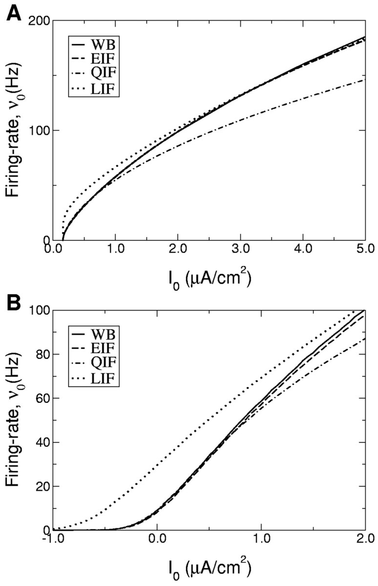
A, B, f-I curves of the LIF, QIF, EIF, and WB neurons for a constant input current (A) and a noisy input current (B) (Gaussian white noise, σ = 5 mV). The parameters of the EIF model were chosen to match the f-I curve of the WB model. The parameters of the QIF model were chosen to match the behavior of the f-I curve of the WB model near firing onset. The range of firing rates in which the f-I curves of the QIF and WB models match is more restricted than for the EIF model. The f-I curve of the LIF neuron cannot be made to agree with the f-I curves of the other models at low firing rates because of the different qualitative dependence of the firing rate on the input current (logarithmic vs square-root). In contrast, the parameters of the LIF model can be determined to match the f-I curve of the WB model at high frequencies (see Materials and Methods for details on the determination of the model parameters).

Fokker-Planck equation. To analyze the response of an IF neuron to a time-dependent input, we studied how the distribution of its voltage, P(V, t), evolves over time. We assumed Gaussian white noise, I_noise(t) = σ √C_gL η(t), where η(t) has unit variance and σ has a dimension of a voltage. The distribution, P(V, t), at time t obeys the Fokker-Planck equation (Risken, 1984; Abbott and van Vreeswijk, 1993; Brunel and Hakim 1999; Brunel, 2000; Knight et al., 2000; Nykamp and Tranchina, 2000; Brunel et al., 2001; Fourcaud and Brunel, 2002):

11

where

is the probability flux through the potential V (i.e., the probability per unit of time that the membrane potential of the neuron crosses the value V from below at time t). The firing rate, ν, of the neuron is the flux through V = ∞:

12

For a complete analytical description, one also needs the boundary conditions, which take into account that, after the spike, the neuron is reset to V_r.

All of our calculations are based on the above equations, which are valid for white input noise, or on their generalizations for more realistic noise models. The details of the calculations can be found in Appendix B.

Simulations of the EIF model. In the EIF model, an action potential is defined as a divergence of the voltage. In simulations, one has to introduce a cutoff at a finite voltage V_th. However, if one assumes that the neuron immediately spikes after reaching V_th, one ends up with a neuron that is effectively an LIF for some inputs. This can be avoided by treating the spike more carefully. In our simulations, we chose a threshold V_th large enough so that:

13

by a factor ≥100. For V < V_th, we integrated the dynamics using a stochastic RK2 algorithm (Honeycutt, 1992). For V > V_th, we neglected all of the currents but ψ(V) and analytically integrated Equation 6. In particular, the time it takes for the voltage to increase from V = V_th to V = +∞ is t_sp = τ_m exp[(V_T - V_th)/Δ_T]. If V_th is too large, the RK2 procedure at large V underestimates the increase in the membrane potential at each time step. This leads to a systematic overestimate in the spike time and causes an additional phase shift in the neuronal response. In practice, we must make sure the time t_sp is large compared with the integration time step dt. Thus, one needs to check that the two conditions, (Eq. 13) and t_sp >> dt, are both satisfied. In the simulations with Δ_T = 3.48, a value for which both conditions are satisfied with V_th = -30 mV for the range of inputs that we investigated.

Results

Filter of a simple conductance-based model

We investigated how the instantaneous firing rate of the WB model is modulated by a sinusoidal input at frequency f in the presence of a noisy background input using numerical simulations. Figure 2A shows a particular realization of such an input current. The instantaneous firing rate is computed by averaging the response over many realizations of the noise, as shown in Figure 2, B and C. Figure 2, D and E, shows how the amplitude and phase shift of the firing rate modulation of the neuron depends on the frequency of the sinusoidal input when the noisy component is a Gaussian white noise with an SD of σ = 6.3 mV and its DC part is such that the average firing rate is ν₀ = 40 Hz.

Figure 2.

Firing rate modulation of a conductance-based neuron. A, Deterministic part of the input current (dashed line) with input noise (solid line). B, Raster plot, 2000 repetitions of the input current with independent noise sources. C, Instantaneous firing rate of the neuron averaged over these repetitions. D, E, Gain (D) and phase shift (E) of the firing rate modulation of a WB neuron versus the frequency, f, of the oscillating input. Spiking threshold, V_s, is -20 mV (□) and 20 mV (○). The dashed line in D is obtained by fitting the simulated data, assuming a decay proportional to 1/f at high frequencies. The phase shift at high frequencies depends on the definition of the spike time. It increases linearly with f (dotted and dotted-dashed lines are linear fits at high frequencies). In both D and E, error bars are smaller than symbol size. Parameters: σ = 6.3 mV (white noise), ν₀ = 40 Hz.

The amplitude versus frequency curve (Fig. 2D) shows a marked attenuation of the response above a frequency of ∼50 Hz. A fit of our numerical simulation data in the range 50 Hz < f < 500 Hz, assuming a power law decay, reveals that the firing rate modulation at large f decays as 1/f (Fig. 2D). Moreover, we find that in this frequency range, the phase shift does not vary much and is slightly larger than 90°, as shown in Figure 2E. We performed extensive numerical simulations varying the level of noise and the DC external input as well as the temporally correlated noise. In all of these simulations, the same behavior of the firing rate modulation was found at sufficiently large f, although the frequency above which it becomes apparent depends on the values of the varied parameters (Fig. 9).

Figure 9.

Comparison of the filters of the WB model (□) and the EIF model (○). We plot the gain (A, 1-2) and phase shift (B, 1-2) with high (A-1, B-1) and low noise (A-2, B-2). Note the good agreement in all regimes for the gain. The phase shifts of both models are very similar up to an input frequency at ∼100 Hz in which the WB model has an additional phase lag. This is a consequence of the fixed delay between EIF and WB spike time shown in Figure 3B.

In all of these simulations, the instantaneous spike rate was computed using a definition of spike time as the time the membrane potential crosses a voltage, V_s = 20 mV, from below. The response modulation amplitude does not depend on the precise value of V_s, provided it is sufficiently high (more than -30 mV). In contrast, the phase shift is more sensitive to V_s, especially at very high input frequencies where the increase of the phase shift is linear with a slope that depends on V_s (Fig. 2E).

Integrate-and-fire models with intrinsic spike generation mechanisms

Recent studies have shown that the high-frequency response of the LIF model depends on the temporal correlations of the noise. For white noise, the response decreases as 1/√f with a phase lag of 45°; for colored noise, the response stays finite with no phase lag (Brunel et al., 2001; Fourcaud and Brunel, 2002). These results are clearly at odds with what we found in the simulations of the WB model.

To understand the origin of the behavior of the WB model at high frequencies and why it is different from the LIF, we studied nonlinear integrate-and-fire neurons, in which the membrane potential obeys Equation 6. The advantage of using this simplified model is that it allows us to compute analytically both the f-I curve and the firing rate modulation at high frequencies, and hence to understand in detail the factors that affect it.

With a supralinear spike-generating current ψ(V), the neuron is endowed with an intrinsic mechanism for spike initiation. We considered two cases in particular, the QIF neuron defined by Equation 9 and the EIF neuron defined by Equation 10. These two neuronal models are type I, like the WB model, and their f-I curve increases proportionally to √^I-I_T, near the firing onset at current threshold, I_T. Hence, for both the QIF and EIF, the parameters can be chosen so that the onset of firing in response to a constant input reproduces the parameters of the WB model sufficiently close to the current threshold (Fig. 1) (see Materials and Methods for details). For the EIF model, this constraint determines the value of the “spike slope factor,” Δ_T. To determine the remaining free parameters, V_r and τ_ref, we also required a good fitting of the WB model f-I curve outside the region of bifurcation.

The f-I curves of the QIF and EIF, with parameters so defined, and the WB model are compared in Figure 1A. It shows that the firing rate response to constant current of the EIF and WB models are very close in a broad range of firing rates (up to 200 Hz). The QIF neuron reproduces the f-I curve of the WB neuron well at low firing rates but not at high rates. Finally, the LIF neuron cannot reproduce the f-I curve of type I neurons well at low rates, because the firing rate has a logarithmic, not square root, dependence on I - I_T. However, the LIF neuron can be made to reproduce the f-I curve reasonably well at high firing rates by a suitable adjustment of parameters.

We then compared the response of the QIF, EIF, LIF, and WB models to noisy input currents (Eq. 3, with I₁ = 0). The corresponding f-I curves are plotted in Figure 1B for the four models with the same parameters as in Figure 1A. As in the noiseless case, the f-I curves of the QIF and EIF models match the WB model f-I curve very well in a broad range of input currents, and this range is larger for the EIF model than for the QIF model.

For a more in-depth look at the spiking dynamics of these various models, Figure 3 plots the voltage traces of the four models for the same realization of the input current. As shown in Figure 3A, the QIF, EIF, and LIF models behave on large time scales in a very similar way as the WB model. However, differences between these models are found on shorter time scales, as shown in Figure 3B. The best match with the WB model is obtained with the EIF model. The subthreshold potential traces are essentially indistinguishable. This is because the same leak current is present in both models and because the I-V curves of the two models are very similar near threshold voltage, V_T. The latter property stems from the fact that the activation curve of the fast sodium current in the WB model can be well approximated near threshold by an exponential function, as shown in Figure 3C. Thus, the membrane potential behavior at the spike onset is very similar for the WB and EIF models. After initiation, the dynamics of the spike in the WB model is controlled by the interplay between Na⁺ and K⁺ channel dynamics and is essentially independent of synaptic inputs. Thus, its spike shape is approximately invariant. Consequently, the only significant difference between the EIF and WB models, the precise shape of the spike after the onset, leads to an input-independent fixed short delay (of order 0.1-0.2 msec) between the spikes of the two models.

Figure 3.

A, Voltage traces for WB, EIF, QIF, and LIF neurons for the same realization of the noisy input current. B shows a higher resolution for a short time interval in which a spike has been generated in all models. The subthreshold traces are similar for all models; however, the dynamics of the spike are different on an msec time scale. When the fluctuation leads to a spike in all models, the LIF neuron spikes first. The EIF neuron spikes almost exactly at the spike onset of the WB. The QIF neuron fires much later. For details of the QIF and EIF parameters, see Materials and Methods. For the WB parameters, see Appendix A. Here, the LIF model has the leak current of the WB model, a reset potential of V_r = - 68 mV, and V_th = - 57 mV, to get the same average firing rate as the WB model. C, I-V curve of the EIF (solid line) and WB (dotted line) neurons. The threshold V_T is defined as the minimum of the curve. The spike slope factor Δ_T is proportional to the radius of the curvature of the I-V curve at its minimum.

The other two models failed to reproduce the dynamics of spike initiation of the WB model. When a fluctuation in the input current induces a spike in all four models, the LIF neuron, which has an instantaneous spike, usually spikes first. The spike in the QIF neuron usually occurs later because of the long time spent by the neuron in the voltage threshold.

The high-frequency response of nonlinear integrate-and-fire neurons

We analytically calculated the firing rate response of a general IF model to a sinusoidally modulated input in the presence of Gaussian white noise (Eq. 3). The details of the calculations, which rely on the Fokker-Planck equation and an expansion of both instantaneous firing rate and membrane potential distribution in powers of 1/f, are described in Appendix B. There, we prove that, depending on the function ψ(V), there are three classes of possible behaviors for the firing rate modulation at high frequencies:

1. If ψ′(V)/ψ(V) does not vanish and is finite at large V, the phase lag ϕ(f) is 90°, whereas the response modulation is given by:

   14

   where ψ′(V) is the derivative of ψ. This happens if the spike-generating current has an exponential dependence on the voltage, as in the EIF model. For this model, one finds that at high frequencies:

   15

   and the phase lag is ϕ = 90°.

2. If ψ′(V)/ψ(V) goes to zero at large V, the rate modulation decays faster than 1/f at high frequencies. This is, for instance, the case of the QIF model for which the calculation of the order 1/f² in the expansion of ν₁ shows that at high frequencies, ν₁(f) ≈ (ν₀I₁)/[g_LΔT(2πfτ_m)²], and the phase lag is ϕ = 180° (see Appendix B).

3. If ψ′(V)/ψ(V) diverges when V goes to infinity, the response is less attenuated than 1/f. This happens in particular for the LIF neuron.

We also show in Appendix B that in cases 1 and 2, the high-input frequency behavior is independent of the temporal correlations of the noise. In contrast, in case 3, the properties of the noise matter, as found in previous work in which the LIF model was studied (Brunel et al., 2001; Fourcaud and Brunel 2002). Furthermore, it can be shown that the results hold for current-based as well as conductance-based noise, because in the case of suprathreshold membrane potential, the spike-generating current ψ(V) dominates the neuronal dynamics, and the synaptic input has little effect on what happens after spike initiation.

In conclusion, the amplitude of the firing rate modulation behaves at high frequencies like a power law ν₁(f) ≈ 1/f^α, where the exponent α depends on the nonlinearity of the spike-generating current ψ(V). The phase lag at high-input frequency is απ/2. The exponent α and asymptotic phase shift of the various models are summarized in Table 1. The high frequencies behaviors of the rate modulation in WB and EIF models are extremely consistent. Other IF models failed to reproduce the behavior of the WB model.

Table 1.

High-frequency properties of linear and nonlinear integrate-and-fire models

Model	Exponent α	Phase lag Φ(f → ∞)
LIF, colored noise	0	0
LIF, white noise	0.5	45°
EIF, all types of noise	1	90°
QIF, all types of noise	2	180°

The amplitude of response modulation in the high-frequency regime is proportional to 1/f^α. Note that the types of noise considered include current-based as well as conductance-based synaptic inputs.

Properties of the EIF neuron at intermediate frequencies

The simulation and analytical results described so far show that in the limit of low- and high-input oscillation frequencies, the behaviors of the EIF and WB models are very similar. We consider now the behavior of the EIF model at intermediate frequencies using numerical simulations.

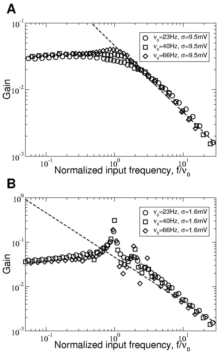
When the noise level is weak, resonances appear at frequencies that are integer multiples of the average firing rate ν₀, f = kν₀ (k = 1, 2,...) (Fig. 4, insets). This is because at low noise levels, the neuron behaves like an oscillator. When the noise increases, the neuronal firing process becomes less regular. The resonant peaks become less pronounced and they disappear, one after the other. For a sufficiently high noise level, the last resonance peak (k = 1) disappears, and the firing rate modulation monotonically decreases with the input frequency, f. The dashed line in Figure 4, computed by numerical simulations, represents the boundary in the plane (ν₀, σ) between the weak noise regime (below the line) where the firing rate modulation displays resonances and the strong noise regime (above the line) where the resonances are completely suppressed. In the latter region, the spike response modulation, ν₁(f), is approximately constant in some range of input frequencies, beyond which it decreases with f with an asymptotic decay in 1/f. Therefore, when the noise is sufficiently large, the EIF neuron behaves like a low-pass filter.

Figure 4.

The qualitative behaviors of the firing rate modulation of the EIF model at intermediate frequencies depend on the characteristics of the input current. Insets show a representative example of the corresponding behavior (gain vs input frequency in log-log scale). In all insets, we plot a simulation of the EIF model (squares, gain) and the EIF and QIF high input frequency regimes (solid and dotted-dashed lines). The dashed line gives the noise level below which there are resonant peaks at the average firing rate ν₀ and possibly at integer multiples of ν₀ in response. Above the dashed line, the EIF model behaves like a low-pass filter, with approximately constant gain at low frequencies and a 1/f attenuation for sufficiently high frequencies. The gain reaches the asymptotic behavior from above at low firing rates, whereas it reaches the asymptotic behavior from below for high firing rates and high noise (see differences in the two insets in the high noise region).

The gain and phase shifts of the filter in the presence of white noise are plotted in Figure 5, A and B, respectively, for fixed ν₀ and three values of the spike slope factor, Δ_T. In all cases, the gain of the filter decreases as 1/f at large enough frequencies. This asymptotic regime is reached earlier for larger Δ_T. There is an overall reduction of the gain as Δ_T increases. This effect is in agreement with our analytical calculation (Eq. 15), which predicts that in the limit f → ∞, the firing rate modulation, ν₁, decreases with Δ_T. This is also consistent with Equation 5, because one can show (using Eq. 29) that the derivative of the f-I curve at ν₀ = 20 Hz is a decreasing function of Δ_T. The phase shift is an increasing function of Δ_T, as shown in Figure 5B. This corresponds to what is expected intuitively, because a decrease of Δ_T increases the sharpness of spike initiation. At large frequencies, the phase shift of the filter goes to -π/2 for any Δ_T, but the convergence is slower when Δ_T is small.

Figure 5.

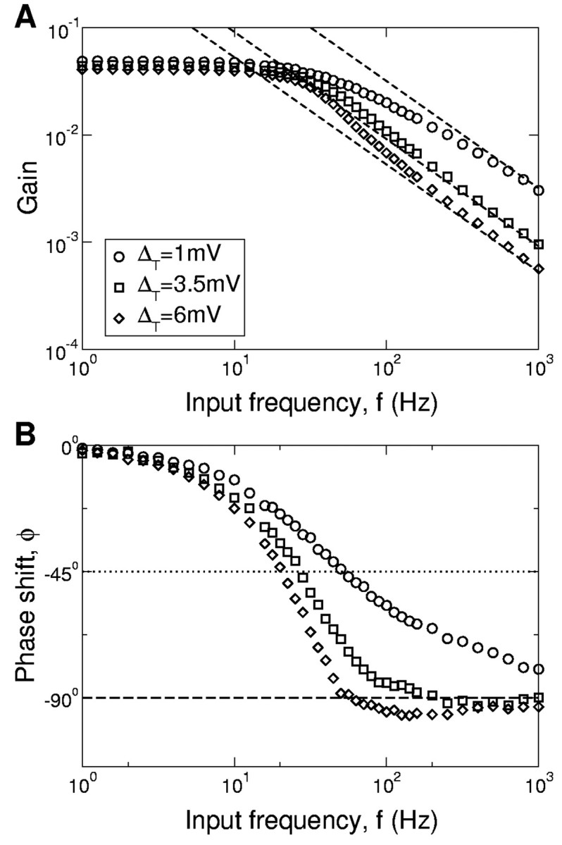
Influence of the spike sharpness on the EIF filter. A, B, Gain (A) and phase (B) of the firing rate modulation are plotted for different values of the spike slope factor Δ_T, indicated in A. Other parameters: ν₀ = 20 Hz, σ = 6.3 mV. Note that as Δ_T decreases, the high frequency asymptotic regime is shifted to higher input frequencies. For large Δ_T, the gain decays faster than 1/f, and the phase shift is larger than 90° in an intermediate frequency range.

Figure 6 shows the effect of temporal correlations in the input noise on the shape of the filter. The response is plotted for three values of the temporal correlation of the noise, τ_s, over a broad range of input frequencies, f. In these simulations, the noise level was adjusted so that the low-frequency response stays constant as τ_s was varied. All three curves overlap for sufficiently large frequencies, f > 100 Hz, in agreement with our analytical results. In contrast, for intermediate frequencies, 30 < f < 100 Hz, the response modulation increases with τ_s. This effect is reminiscent of the behavior of the LIF neuron (Brunel et al., 2001) for which correlations in the input noise suppresses the attenuation of the response modulation (Brunel et al., 2001; Fourcaud and Brunel, 2002).

Figure 6.

Influence of noise correlation time on the gain of the EIF neuron. The stationary firing rate is ν₀ = 30 Hz, and the noise level is adjusted so that the low-frequency response is constant as the synaptic decay time, τ_s, is varied from 0 msec (white noise) to 20 msec.

To further characterize the filtering properties of the neuron, we defined the filter cutoff as the frequency, f_c, for which the filter gain decreases by a factor 1/√2 compared with its low-frequency limit, ν₁(f_c) = ν_LF/√2. We used numerical simulations to study how f_c depends on the average firing rate, ν₀, the spike slope factor, Δ_T, and the temporal correlations in the noise. Figure 7 shows the results for a noise level σ = 8 mV. For this value of σ, the EIF neuron is in the strong noise regime in the entire range of average firing rates and the spike slope factor explored.

Figure 7.

A, B, Cutoff frequency of the EIF filter in the high-noise regime as a function of the firing rate (A) and spike slope factor (B). In A, the parameters of the EIF model are chosen to match the WB model (Δ_T = 3.48 mV). In B, δ_T is varied. In both panels, σ = 8 mV. A, The cutoff frequency is approximately proportional to the average firing rate ν₀ (simulations with white noise). B, The cutoff frequency depends weakly on the slope factor Δ_T for white noise but strongly increases when δ_T decreases for colored noise (ν₀ = 24 Hz; values of the synaptic time constants are indicated in the legend).

Figure 7A shows that for a fixed value of the slope factor, f_c is finite in the limit of low average firing rate, ν₀, and that it is an increasing function of ν₀. For ν₀ > 10 Hz, f_c varies linearly with ν₀. In Figure 7B, the cutoff frequency is displayed as a function of Δ_T for fixed ν₀ and different values of τ_s, the noise correlation time. In general, f_c is a decreasing function of Δ_T but, at large enough Δ_T, it saturates toward a value that depends only weakly on τ_s. In contrast, the smaller the τ_s, the weaker the variations of f_c at small Δ_T. In particular, for white input noise, f_c is almost constant in all of the explored range of Δ_T. Temporal correlations in the noise increase the cutoff frequency, f_c, and this effect is more pronounced at smaller values of Δ_T (i.e., when spikes have sharper initiation).

Domain of validity of the linear response

In the previous sections, we analytically computed the linear response of the EIF neuron to modulated input in the limit of small or large modulation frequency, f. These results should provide a correct quantitative description of the neuron dynamics in these limits for sufficiently weak amplitude modulation, I₁. The numerical simulations presented above, performed for a finite but small value of I₁, confirm this expectation. They also extend our study by investigating the neuronal linear filter at intermediate values of the input frequency.

How large can the input modulation be for the response of the neuron to still be linear? To address this issue, we performed simulations at various levels of input modulation and measured the amplitude of the Fourier components of the response up to order 3. Results of these simulations are displayed in Figure 8 for σ = 6.3 mV, ν₀ = 20 Hz, and an input modulation frequency of f = 20 Hz. For these parameters, ν₁ varies linearly with I₁, and higher order Fourier components are negligible up to input modulations that induce temporal variations of the firing rate as large as 75% of the average firing rate. This shows that the neuron responds in a linear manner in this range of firing rate variations. A similar range of validity was obtained for all values of f tested (0-100 Hz) in the strong noise regime (the boundaries of strong and low-noise regimes are indicated in Fig. 4). In the low-noise regime, the domain of validity is on the same order of magnitude, except for frequencies close to resonances.

Figure 8.

Amplitude of the first three Fourier components of the response, normalized by the average firing rate, ν₀, as a function of the strength of input modulation. Circles, First Fourier component; squares, second Fourier component; diamonds, third Fourier component. Parameters: σ = 6.3 mV; ν₀ = 20 Hz; f = 20 Hz. The first Fourier component, ν₁, is linear in I₁ up to modulations of the firing rate of order ν₀. The higher Fourier components are negligible up to approximately the same amount of modulation. Note that all simulations presented in this study (except in this figure) are done with ν₁ /ν₀ ≈ 0.25, well into the domain of validity of the linear approximation.

Comparison of the linear responses of EIF and conductance-based neurons

In Figure 9, we compare the gain and phase shifts of the EIF and WB models for two levels of noise, σ, and average firing rates, ν₀. We found a remarkable agreement for the gain of the two models in all ranges of frequencies studied. For the phase shift, the agreement is also excellent but in a smaller range of frequencies, up to 100 Hz. Above 100 Hz, the phase lag is significantly smaller in the EIF model than in the WB model. This is a consequence of the delay δ ≈ 0.2 msec between the spikes in the EIF and WB models, which is clearly visible in Figure 3B. The corresponding additional phase lag is 2πfδ. This phase shift depends on the voltage V_s, which is used for the definition of the spike times in the WB model.

In Figure 10, we show how the instantaneous firing rate of WB and EIF models responds to a current step that brings the neuron from 20 to 30 Hz. Again, the figure shows an excellent agreement of EIF and WB model responses, as expected from Figures 8 and 9.

Figure 10.

Comparison of the response of the WB (solid line) and EIF (dashed line) models to a current step (average, >1,600,000 repetitions; firing rate computed in 0.6 msec bins; σ = 6.3 mV). The time course of the responses of WB and EIF models is indistinguishable. The agreement between both models is excellent, confirming the close match of the linear filters shown in Figure 9.

Effect of sodium channel activation kinetics on high-frequency behavior

Sodium channels have a voltage-dependent activation time constant on the order of 0.1 msec (Martina and Jonas, 1997). The WB model makes the simplifying assumption that the sodium activation is instantaneous. Because ψ(V) depends on the voltage directly in the nonlinear IF models, the effective spike initiation is also instantaneous in these models. In most situations, this assumption will not affect the results much, but there is clearly a frequency above which the finite activation time constant will become important.

To measure at which frequency the activation kinetics affects the firing rate modulation, we introduced the activation kinetics in the WB model as in the Hodgkin-Huxley formalism. For the EIF model, we replaced the spike-generating current, ψ(V), by a dynamical variable with an activation time constant, τ_act = 0.1 msec: τ_actdψ/dt = -ψ + g_LΔT exp[(V - V_T)/Δ_T]. After each spike, the potential was reset to V_r, and the spike-generating current was reset to ψ(V_r). Results are shown in Figure 11. In both models, the firing rate modulation was not affected at low and intermediate frequencies. It was only slightly more attenuated and had a larger phase lag at input frequency beyond several hundred Hertz. In particular, the cutoff frequency was not affected, and the instantaneous model was sufficient to describe the neuron dynamics in a wide range of input frequencies (0-500 Hz). Slower activation kinetics decreased the frequency at which the deviation from the 1/f behavior occurred. For example, for time constants of 1 msec, the response is already significantly more attenuated than 1/f below 100 Hz.

Figure 11.

Gain of the firing rate modulation of EIF and WB models with noninstantaneous sodium activation kinetics. The dashed line shows the asymptotic regime for an instantaneous activation. The activation kinetics attenuates the response slightly more only for frequencies beyond several hundred Hertz.

High-frequency behavior of other conductance-based neurons

So far, our results suggest that the high-frequency response depends only on the properties of the current leading to spike generation. To test this prediction, we performed numerical simulations of a conductance-based model with the same fast sodium current as in the WB model but with several additional ionic currents (Hansel and van Vreeswijk, 2002) (see Materials and Methods). These additional currents modify the subthreshold behavior of the neuron and act on time scales slower than the sodium activation time. They have a significant effect on the response at low-input frequencies because of, in particular, the adaptation current. However, Figure 12 shows that, above the cutoff frequency, the amplitude of the firing rate modulation decreases again as 1/f as in the EIF model. The dashed line in Figure 12 shows the amplitude in the asymptotic regime predicted by the EIF neuron (Eq. 15) with the same values of C and Δ_T as for the regularly firing and WB neurons. This confirms that high-input frequency behavior is determined only by intrinsic currents leading to spike emission and the average firing rate.

Figure 12.

Amplitude of the firing rate modulation for a conductance-based model with additional currents. A, B, Response to inputs with strong (A) and weak (B) noise and various average firing rates (indicated in corresponding panels). The high frequency behavior is proportional to 1/f with a cutoff close to the average firing rate, ν₀. The dashed line shows the EIF high-input frequency asymptotic regime with parameters matching the sodium activation curve of the conductance-based neuron. Note that in this figure, the frequency is normalized to the average firing rate, ν₀, so that all response curves match approximately at high frequencies. The 1/f regime extends up to 1000 Hz as in the WB model.

Discussion

We studied how the firing rate response of a neuron to an oscillating input depends on the modulation frequency, f. The models that we investigated include conductance-based models as well as generalized integrate-and-fire models. For sufficiently strong noise, we found that these neurons behave like a low-pass filter. For f below a cutoff frequency f_c, the response modulation is weakly dependent on f. For f > f_c, it decreases rapidly with f and behaves at large f like a power law C/f^α, where C is a prefactor independent of f. We analytically calculated α and C for generalized integrate-and-fire models and have shown that α depends on the nonlinearity of spike initiation.

Of particular interest is the case of neurons with an exponential spike nonlinearity (EIF model). In this case, α = 1, and C depends on both the average firing rate of the neuron and the sharpness of spike initiation characterized by the spike slope factor, Δ_T. This high-frequency behavior is independent of the properties of the noise; it holds for white noise as well as colored noise and for current-based and conductance-based noise. In contrast, all other types of nonlinearity lead to exponents α different from 1.

Fast sodium currents involved in action potentials increase exponentially near firing onset. Therefore, we expect that our analytical results derived in the framework of the EIF are relevant to predicting the response of real neurons to rapidly varying inputs. This is further supported by our simulations of conductance-based models, the quantitative behavior of which is identical to that found for the EIF.

We have also shown that the cutoff frequency of the EIF neuron increases approximately linearly with the average firing rate, and that it is a decreasing function of the spike slope factor Δ_T. The latter dependency is very mild for white noise but much more pronounced for colored noise. We expect this result to be generic, as confirmed by our simulations of simple conductance-based models.

Implications for modeling

We have shown how a simple conductance-based neuronal model can be reduced in a systematic way to a new type of integrate-and-fire model, the EIF model, in which the dynamics involve a current that increases exponentially with the membrane potential. Remarkably, the responses to rapidly fluctuating inputs of the full and reduced models are indistinguishable. More generally, the filter characteristics are quantitatively similar for the two models in the entire range of input frequencies. This is in contrast to the LIF model, the response properties (Gerstner, 2000; Brunel et al., 2001; Fourcaud and Brunel, 2002; Mazurek and Shadlen, 2002; van Rossum et al., 2002) of which differ qualitatively from those of conductance-based models at all frequencies, as shown here. Also, although QIF and conductance-based neurons behave similarly at low frequencies, qualitative discrepancies remain at high frequencies.

The stability of asynchronous firing in large networks of interacting neurons has been studied extensively in LIF (Abbott and van Vreeswijk, 1993; Treves, 1993; Brunel and Hakim, 1999; Brunel, 2000) and QIF (Hansel and Mato, 2001, 2003) neuronal networks. The approach developed in these studies can be generalized to some extent for neurons with more realistic dynamics, provided that one knows how they respond to weakly modulated oscillating inputs. Hence, the present study paves the way for a greater understanding of the synchronization properties of conductance-based neurons. In particular, the presence of a cutoff frequency in the filtering properties of conductance-based neurons indicates that there is an upper bound to the frequency of population oscillations, which can emerge in large networks (Geisler et al., 2002).

Functional implications

Our results can be used to determine how many neurons are needed to detect a transient signal in noisy conditions, given single-neuron characteristics. Equivalently, one can calculate the minimal duration a given signal should last to be detected. Consider, for example, a population of 100 neurons emitting at a background rate of 10 Hz and subjected to a transient signal that, if applied for a time long enough, would increase the firing rate to 20 Hz. An ideal detector must be able to distinguish the transient increase of the population rate induced by the signal from rate fluctuations attributable to the finite number of neurons. This can be done using a receiver operator characteristics analysis (Green and Swets, 1966). Briefly, one computes the distributions of the spike counts in a given interval under two conditions (signal or no signal). One then computes the probability of correct detection of the signal (i.e., the probability that the spike count is larger when the signal is present than when it is absent). If neurons have very sharp spikes (Δ_T close to zero) in the presence of correlated noise, the signal can be detected in ∼5 msec with 90% accuracy. If the spike slope factor is Δ_T = 3 mV, the signal can be detected only in ∼12 msec with the same accuracy. The detection time increases further for larger values of Δ_T.

Experimental implications

How sharp are spikes in cortical neurons?

Our work shows that the spike slope factor, Δ_T, is one of the main parameters on which the response of a neuron to fluctuating inputs depends. Activation curves of Na⁺ channels have been measured in several preparations, including neocortical pyramidal cells (Fleidervish et al., 1996), hippocampal pyramidal cells, granule cells, and basket cells (Martina and Jonas, 1997; Fricker et al., 1999; Ellerkmann et al., 2001). These authors used Boltzmann functions to fit the observed data. Using their best-fit parameters, one finds Δ_T in the range of 3-6 mV for these types of cells. However, in all cases, there are few data points in the region of the threshold, leading to a considerable uncertainty in the estimate of this parameter. Therefore, more experiments are needed to determine the spike slope factor of cortical neurons.

Experimental measurements of the linear response of neurons

The instantaneous firing rate of neurons responding to sinusoidal currents has been measured in slice preparations (Knight, 1972b; Carandini et al., 1996; Chance, 2000). Carandini et al. (1996) and Chance (2000) found cutoff frequencies in the range of 10-100 Hz that increase with the average firing rate. This is consistent with our findings. However, none of these studies have systematically explored high-frequency behavior. Bair and Koch (1996) measured the poststimulus time histogram power spectra of MT neurons in response to visual stimuli consisting of randomly moving dots. In the examples shown in this study, the output power spectrum is rapidly attenuated in the 30-100 Hz frequency range. However, it is difficult to interpret these results, because the frequency content of the synaptic input to MT neurons is unknown. Thus, additional experiments are needed to test our prediction for the 1/f attenuation of the response at high frequencies.

Testing our experimental predictions

The main predictions of our work are: (1) the neuronal gain decays as 1/f at high frequency, independently of the characteristics of the input, (2) the cutoff frequency increases with the average firing rate, and (3) the cutoff frequency increases when the spike slope factor decreases in the presence of temporally correlated noise. One possible experimental test of these results would be to study the response of neurons in vitro, in which sodium channels underlying spike initiation are blocked with TTX and replaced, using dynamic clamp techniques by an artificial sodium current with known properties. Note that because the dynamics of sodium currents underlying spike initiation are fast, a dedicated analog circuit may be needed to emulate them with the dynamic clamp method. A similar experiment can be devised in vivo (e.g., in cortical neurons). Using QX314 (lidocaine N-ethyl bromide quaternary salt) intracellularly, sodium currents in a specific cell can be blocked without affecting the activity of its neighboring cells. This would preserve the background noise that the cell receives from the rest of the network and allow for the study of its effect on the response.

Appendix

A. Conductance-based models

The Wang-Buszáki model was introduced by Wang and Buzsáki (1996). The membrane potential V(t) is governed by the following equation:

where C_M is the membrane capacitance (C_M = 1 μF/cm²), I_L = g_L(V - V_L) is the leak current (g_L = 0.1 mS/cm²; V_L = -65 mV; τ_m = C/g_L = 10 msec), I_Na = g_Nam³h(V - V_Na) is the sodium Hodgkin-Huxley current with an instantaneous activation variable, I_K = g_Kn⁴(V - V_K) is the delayed rectifier potassium current, and I_syn(t) is the input current defined in Materials and Methods.

The dynamical equations for the gating variables are:

16

where x = m, h, n. All functions x_∞(V), τ_x are given in Table 2. The respective maximum conductance densities and the reversal potentials of the ionic currents are given in Table 3.

Table 2.

Gating variables of conductance-based models

X	ax	bx
m		4 exp [-(V + 60)/18]
h	0.35 exp[-V + 58)/20]
n		0.625 exp[V + 44)/80]
X	X∞	τx
a		Instantaneous
b		20
s		Instantaneous
Z		50

, and for X=m, h, n; a_x and b_x in msec^-1; τ_x in msec.

Table 3.

Conductance density in mS/cm² and reversal potentials in mV for the ionic channels in the conductance-based models

X	gx	Vx
Na	35	55
NaP	0.08	55
K	15	−90
A	2.5	−90
K5	0.5	−90

Another conductance-based model used in this work is taken from Hansel and van Vreeswijk (2002). The dynamics of the model are described by:

17

where the currents I_L, I_Na, and I_K are identical to the WB model (except V_L = -70 mV), but three additional ionic currents are present: (1) a persistent sodium current, I_NaP = g_NaPs_∞(V) (V - V_Na), (2) an A-type potassium current, I_A = g_Aa_∞(V)³b(V - V_K), and (3) a slow potassium current responsible for spike adaptation, I_Ks = g_Ksz(V - V_K).

The dynamical equations for the gating variables m, h, n, b, and z are given by Equation 16. All gating variable parameters are given in Table 2. The respective maximum conductance densities and the reversal potentials of the ionic currents are given in Table 3.

In most of this study, we neglect the sodium activation kinetics, and we take m = m_∞.

B. Analytical calculations of the neuronal response to sinusoidal modulated noisy inputs

B1. Gaussian white noise

We rewrite Equation 6 as:

18

with F(V)=-V+V_L+ψ(V)/g_L and:

19

20

where I(t) is the deterministic part of the input current, and η(t) is a Gaussian white noise with zero mean and unitary SD. The frequency of the modulation is f and ω ≡ 2πf. For convenience, we also define μ(t) = I(t)/g_L, which can be written as μ(t) = μ₀ + μ₁ cos(ωt), with μ₀ = I₀/g_L, μ₁ = I₁/g_L. We denote the membrane time constant τ_m = C/g_L. Equation 18 can then be rewritten as:

21

The distribution of voltages at time t obeys the Fokker-Planck equation (Risken, 1984):

22

with the boundary conditions: The reset of the voltage to V_r after the spike is taken into account by requiring that:

23

We solve this equation assuming that μ₁ << μ₀. For the sake of simplicity, we use complex notations and write to first order:

24

where P₁(V, ω), ν₁(ω), and J_V,1(V, ω) are complex quantities,|P₁| << P₀,|ν₁| << ν₀,|J_V,1| << J_V,0.

25

Substituting Equation 24 in Equation 22 and keeping only the terms at leading order, one finds that P₀(V) satisfies the equation:

26

which, after one integration over V, gives: where K₊ and K_- are constants. The boundary condition (Eq. 12) and reset (Eq. 23) determine K₊ and K_-:

27

The solution of Equation 26 is:

28

The normalization of the distribution P₀(V) determines the average firing rate, ν₀. One finds:

29

We now consider the first order contributions in the expansions of Equation 22. One finds:

30

The boundary condition at the same order gives:

31

In the last equality, we used the fact that F(V) goes to infinity at large V.

The solution of Equations 30 and 31 simplifies in two limits:

Low-input frequency

At low frequencies (ωτ_m << 1), P(V, t) follows adiabatically the slowly changing input, and the left-hand side of Equation 30 can be neglected. It is then easy to check that is a solution of Equation 30. Using P₀(V) ≈_V→∞ ν₀/F(V) (Eqs. 26, 31), we can compute the firing rate modulation in the low-input frequency limit:

32

High-input frequency

Expanding Equation 30 in powers of 1/ω and keeping only the leading order gives:

33

and ν₁ is determined by the large V behavior of P₁(V) (Eq. 29). Using Equation 26 and the fact that F(V) diverges at large V, one finds:

34

and thus

35

Inserting Equation 35 into Equation 33, we find:

36

Finally, inserting Equation 36 into Equation 31, we find:

37

This formula can be applied to the EIF model to show that ν₁ decays like 1/ω at large ω. In contrast, for any polynomial F(V), the 1/ω term vanishes, and it is necessary to calculate P₁ and ν₁ at the next order (i.e., 1/ω ²). One finds that ν₁ = A/ω², where the prefactor A is proportional to lim_V→∞(F′² - FF″)/F. In particular, if F ≈ V² at large V, A is finite, and ν₁ decays like 1/ω² at large ω. This is the case for the QIF model for which one finds:

38

If F ≈ V^k > 2 at large V, A diverges. In this case, one expects the firing rate modulation to decrease like 1/ω^α with 1 < α < 2.

B2. Temporally correlated noise

In the previous section, we assumed white Gaussian input noise. Here, we show that the presence of correlations does not affect the high-frequency behavior of the spike response modulation of the EIF neurons. Assuming that synaptic current decays exponentially with a synaptic time constant, τ_s, the equations for the dynamics of the IF neurons are:

The probability density function, P(V, μ_syn,t) (Brunel et al., 2001; Haskell et al., 2001; Fourcaud and Brunel, 2002), satisfies a two-dimensional Fokker-Planck equation:

39

The probability flux is now a two-dimensional vector with components:

40

41

In particular, in the large V limit:

42

because F(V) diverges at large V. As before, the instantaneous firing rate is given by:

43

To solve these equations, one expands P(V, μ_syn,t), J_V(V, μ_syn,t) and ν(t) in a way similar to the case of white noise. One finds:

44

and

45

for k = 0, 1. A similar analysis, as in the white noise case, shows that at first order in 1/ω:

46

Combining Equations 44-45, one can show that:

47

48

which is the same expression as in the case of white noise (Eq. 37). Therefore, the asymptotic behavior at high frequencies of the instantaneous rate modulation is not affected by the presence of temporal correlations in the noise.

References

- Abbott LF, van Vreeswijk C ( 1993) Asynchronous states in a network of pulse-coupled oscillators. Phys Rev E Stat Phys Plasmas Fluids Relat Interdiscip Topics 48: 1483-1490. [DOI] [PubMed] [Google Scholar]
- Bair W, Koch C ( 1996) Temporal precision of spike trains in extrastriate cortex of the behaving macaque monkey. Neural Comput 8: 1185-1202. [DOI] [PubMed] [Google Scholar]
- Brunel N ( 2000) Dynamics of sparsely connected networks of excitatory and inhibitory spiking neurons. J Comput Neurosci 8: 183-208. [DOI] [PubMed] [Google Scholar]
- Brunel N, Hakim V ( 1999) Fast global oscillations in networks of integrate-and-fire neurons with low firing rates. Neural Comput 11: 1621-1671. [DOI] [PubMed] [Google Scholar]
- Brunel N, Chance F, Fourcaud N, Abbott L ( 2001) Effects of synaptic noise and filtering on the frequency response of spiking neurons. Phys Rev Lett 86: 2186-2189. [DOI] [PubMed] [Google Scholar]
- Carandini M, Mechler F, Leonard CS, Movshon JA ( 1996) Spike train encoding by regular-spiking cells of the visual cortex. J Neurophysiol 76: 3425-3441. [DOI] [PubMed] [Google Scholar]
- Chance F ( 2000) Modeling cortical dynamics and the responses of neurons in the primary visual cortex. PhD thesis, Brandeis University.
- Ellerkmann RK, Riazanski V, Elger CE, Urban BW, Beck H ( 2001) Slow recovery from inactivation regulates the availability of voltage-dependent Na+ channels in hippocampal granule cells, hilar neurons and basket cells. J Physiol (Lond) 532: 385-397. [DOI] [PMC free article] [PubMed] [Google Scholar]
- Ermentrout GB ( 1996) Type I membranes, phase resetting curves, and synchrony. Neural Computation 8: 979-1001. [DOI] [PubMed] [Google Scholar]
- Ermentrout GB, Kopell N ( 1986) Parabolic bursting in an excitable system coupled with a slow oscillation. SIAM J Appl Math 46: 233-253. [Google Scholar]
- Fleidervish IA, Friedman A, Gutnick MJ ( 1996) Slow inactivation of Na+ current and slow cumulative spike adaptation in mouse and guinea-pig neocortical neurones in slices. J Physiol (Lond) 493: 83-97. [DOI] [PMC free article] [PubMed] [Google Scholar]
- Fourcaud N, Brunel N ( 2002) Dynamics of firing probability of noisy integrate-and-fire neurons. Neural Comput 14: 2057-2110. [DOI] [PubMed] [Google Scholar]
- Fricker D, Verheugen JAH, Miles R ( 1999) Cell-attached measurements of the firing threshold of rat hippocampal neurones. J Physiol (Lond) 517: 791-804. [DOI] [PMC free article] [PubMed] [Google Scholar]
- Geisler CM, Brunel N, Fourcaud N, Wang X-J ( 2002) The interplay between intrinsic spiking dynamics and recurrent synaptic interactions in the generation of stochastic network oscillations. Soc Neurosci Abstr 28: 276.12. [Google Scholar]
- Gerstner W ( 2000) Population dynamics of spiking neurons: fast transients, asynchronous states, and locking. Neural Comput 12: 43-89. [DOI] [PubMed] [Google Scholar]
- Green DM, Swets JA ( 1966) Signal detection theory and psychophysics. New York: Wiley.
- Hansel D, Mato G ( 2001) Existence and stability of persistent states in large neuronal networks. Phys Rev Lett 10: 4175-4178. [DOI] [PubMed] [Google Scholar]
- Hansel D, Mato G ( 2003) Asynchronous states and the emergence of synchrony in large networks of interacting excitatory and inhibitory neurons. Neural Comput 15: 1-56. [DOI] [PubMed] [Google Scholar]
- Hansel D, van Vreeswijk C ( 2002) How noise contributes to contrast invariance of orientation tuning in cat visual cortex. J Neurosci 22: 5118-5128. [DOI] [PMC free article] [PubMed] [Google Scholar]
- Haskell E, Nykamp DQ, Tranchina D ( 2001) Population density methods for large-scale modelling of neuronal networks with realistic synaptic kinetics: cutting the dimension down to size. Network 12: 141-174. [PubMed] [Google Scholar]
- Hodgkin AL, Huxley AF ( 1952) A quantitative description of membrane current and its application to conductance and excitation in nerve. J Physiol (Lond) 117: 500-544. [DOI] [PMC free article] [PubMed] [Google Scholar]
- Honeycutt RL ( 1992) Stochastic Runge-Kutta algorithms. I. White noise. Phys Rev A 45: 600-603. [DOI] [PubMed] [Google Scholar]
- Knight BW ( 1972a) Dynamics of encoding in a population of neurons. J Gen Physiol 59: 734-766. [DOI] [PMC free article] [PubMed] [Google Scholar]
- Knight BW ( 1972b) The relationship between the firing rate of a single neuron and the level of activity in a population of neurons. J Gen Physiol 59: 767-778. [DOI] [PMC free article] [PubMed] [Google Scholar]
- Knight BW, Omurtag A, Sirovich L ( 2000) The approach of a neuron population firing rate to a new equilibrium: an exact theoretical result. Neural Comput 12: 1045-1055. [DOI] [PubMed] [Google Scholar]
- Martina M, Jonas P ( 1997) Functional differences in Na+ channel gating between fast-spiking interneurons and principal neurones of rat hippocampus. J Physiol (Lond) 505: 593-603. [DOI] [PMC free article] [PubMed] [Google Scholar]
- Mazurek ME, Shadlen MN ( 2002) Limits to the temporal fidelity of cortical spike rate signals. Nat Neurosci 5: 463-471. [DOI] [PubMed] [Google Scholar]
- McCormick D, Connors B, Lighthall J, Prince D ( 1985) Comparative electrophysiology of pyramidal and sparsely spiny stellate neurons in the neocortex. J Neurophysiol 54: 782-806. [DOI] [PubMed] [Google Scholar]
- Nowak L, Sanchez-Vives M, McCormick D ( 1997) Influence of low and high frequency inputs on spike timing in visual cortical neurons. Cereb Cortex 7: 487-501. [DOI] [PubMed] [Google Scholar]
- Nykamp DQ, Tranchina D ( 2000) A population density approach that facilitates large-scale modeling of neural networks: analysis and an application to orientation tuning. J Comp Neurosci 8: 19-30. [DOI] [PubMed] [Google Scholar]
- Powers RK, Binder MD ( 2001) Input-output functions of mammalian motoneurons. Rev Physiol Biochem Pharmacol 143: 137-263. [DOI] [PubMed] [Google Scholar]
- Ris L, Hachemaoui M, Vibert N, Godaux E, Vidal PP, Moore LE ( 2001) Resonance of spike discharge modulation in neurons of the guinea pig medial vestibular nucleus. J Neurophysiol 86: 703-716. [DOI] [PubMed] [Google Scholar]
- Risken H ( 1984) The Fokker-Planck equation: methods of solution and applications. Berlin: Springer.
- Sekirnjak C, du Lac S ( 2002) Intrinsic firing dynamics of vestibular nucleus neurons. J Neurosci 22: 2083-2095. [DOI] [PMC free article] [PubMed] [Google Scholar]
- Treves A ( 1993) Mean-field analysis of neuronal spike dynamics. Network 4: 259-284. [Google Scholar]
- Tuckwell HC ( 1988) Introduction to theoretical neurobiology. Cambridge: Cambridge UP.
- van Rossum MCW, Turrigiano GG, Nelson SB ( 2002) Fast propagation of firing rates through layered networks of noisy neurons. J Neurosci 22: 1956-1966. [DOI] [PMC free article] [PubMed] [Google Scholar]
- Wang X-J, Buzsáki G ( 1996) Gamma oscillation by synaptic inhibition in a hippocampal interneuronal network model. J Neurosci 16: 6402-6413. [DOI] [PMC free article] [PubMed] [Google Scholar]