Interaural Time Difference Discrimination Thresholds for Single Neurons in the Inferior Colliculus of Guinea Pigs

Abstract

Sensitivity to changes in the interaural time difference (ITD) of 50 msec tones was measured in single units in the inferior colliculus of urethane-anesthetized guinea pigs. ITD functions were measured with 100 repeats and fine spacing (100 points per cycle). The just noticeable difference (jnd) for ITD was determined using receiver operating characteristic (ROC) analysis of the spike-count distribution at each ITD. The jnd became progressively smaller as the signal frequency increased from 50 to 800 Hz but became unmeasurable above 1 kHz. The lowest jnds (30 μsec) were comparable with human jnds, indicating that there is sufficient information in the firings of individual neurons to permit discrimination without obligatory pooling. ROC analysis requires the choice of a reference ITD from which the jnd may be found by stepping the target ITD through the ITD function. For each neuron the reference was chosen to minimize the jnd. The lowest jnd was usually for ipsilateral leading references, near the minimum of the ITD function where the variance was also low, but where the slope was nearing its steepest. This was despite the peak of the ITD function occurring for contralateral leading stimuli. When the reference ITD was on midline, a jnd could be obtained by looking for firing rates either greater or smaller than the firing rate at midline. The lower jnd was usually obtained by looking for a decrease in firing rate. As duration increased, jnds either decreased or increased, depending on unit type, whereas when level increased, jnds generally increased.

Introduction

For humans, the azimuthal localization of sounds below 1500 Hz is mediated primarily by sensitivity to the small difference in travel time to the two ears [interaural time difference (ITD)]. The smallest change in the ITD of pure tones detectable by humans [just noticeable difference (jnd)] is 10–20 μsec (Mills, 1958; Durlach and Colburn, 1978; Hafter et al., 1979). This sensitivity is normally modeled using an array of coincidence detectors, each of which fires maximally when spikes from the two ears arrive at the same time, via axons with different propagation delays, hence showing sensitivity to a particular ITD (Jeffress, 1948). Neurons in the medial superior olive (MSO) behave like coincidence detectors (Goldberg and Brown, 1969; Yin and Chan, 1990; Spitzer and Semple, 1995; Batra et al., 1997a,b). Because the variability in synaptic delay is much larger than the psychophysically determined jnd, it has been widely assumed that jnds as low as those of humans could only be achieved if the responses from many neurons were combined (Hall, 1965; Yin and Chan, 1988; Carr, 1993; Gerstner et al., 1996; Fitzpatrick et al., 1997; Yin et al., 1997).

There are examples, however, where the resolution measurable from single neurons reflects the psychophysical thresholds. Individual neurons in the visual and somatosensory systems carry sufficient information to achieve performance comparable with psychophysical thresholds (Johansson and Vallbo, 1979; Bradley et al., 1985; Parker and Hawken, 1985; Newsome et al., 1989; Hawken and Parker, 1990;Vallbo, 1995). Individual auditory nerve fibers also carry sufficient information to exceed human capability in tone detection and forward masking (Relkin and Pelli, 1987; Relkin and Turner, 1988) and to equal human capability in detecting tones in noise (Young and Barta, 1986). Single goldfish auditory nerve fibers provide for level discrimination that exceeds the animal's behavioral capability, although they do not reach human performance (Fay and Coombs, 1992). In light of these findings, which show that some individual neurons can match psychophysical thresholds, it is important to reexamine the assumption that behavioral ITD jnds require pooling across many cells.

The sensitivity to a change in stimulus is dependent on both the variability in the response to a constant stimulus and the change in response when the stimulus is changed (Green and Swets, 1974). It is therefore vital that, in addition to the mean rate, the distribution of neural spike counts to repeated stimulation is measured. Skottun (1998), using published mean rate responses (Stanford et al., 1992), showed that single inferior colliculus (IC) and thalamic neurons can achieve ITD jnds as small as those obtained in humans. However, he had to make assumptions about the spike distributions. These were subsequently measured in the IC of guinea pigs (Skottun et al., 2001), which confirmed the earlier finding. In this paper, we study in greater detail the ability of single IC neurons to signal differences in ITD. We particularly focus on the effects of unit type, signal duration, signal level, and other factors relating to the comparison between neural and behavioral performance.

Materials and Methods

Recordings were made in the right IC of 15 pigmented guinea pigs weighing 335–507 gm; in many of these experiments data were also collected for other purposes. Animals were anesthetized with urethane (1.3 gm/kg, i.p., in 20% solution in 0.9% saline) and Hypnorm (Janssen, High Wycombe, UK) (0.2 ml, i.m., comprising fentanyl citrate 0.315 mg/ml and fluanisone 10 mg/ml). To prevent bronchial secretions, atropine sulfate (0.06 mg/kg, s.c.) was administered at the start of the experiment. Anesthesia was supplemented with further doses of Hypnorm (0.2 ml, i.m.), on indication of pedal withdrawal reflex. A tracheotomy was performed, and core temperature was maintained at 38°C via a heating blanket and rectal probe. The animals were placed inside a sound attenuating room in a stereotaxic frame in which hollow plastic speculas replaced the ear bars to allow sound presentation and direct visualization of the tympanic membrane. A craniotomy was performed over the position of the IC. The dura was reflected, and the surface of the brain was covered by a solution of 1.5% agar in 0.9% saline. Respiratory rate was monitored by means of a fine polythene tube inserted into the tracheal cannula connected to a low-pressure transducer; heart rate was monitored using a pair of electrodes inserted into the skin to either side of the animal's thorax. All experiments were performed in accordance with the United Kingdom Animal (Scientific Procedures) Act of 1986.

Recordings were made with glass-insulated tungsten electrodes (Bullock et al., 1988) advanced into the IC (optional charge) through the intact cortex, in a vertical penetration, by a piezoelectric motor (Burleigh Inchworm IW-700/710). Extracellular action potentials were amplified (Axoprobe 1A, Axon Instruments, Foster City, CA), discriminated using a level-crossing detector (SD1, Tucker-Davies Technologies), and their time of occurrence was recorded with a resolution of 1 μsec.

Stimuli were delivered to each ear through sealed acoustic systems comprising custom-modified Radioshack 40–1377 tweeters joined via a conical section to a damped 2.5-mm-diameter, 34-mm-long tube (M. Ravicz, Eaton Peabody Laboratory, Boston, MA), which fit into the hollow speculum. The output was calibrated a few millimeters from the tympanic membrane using a Brüel and Kjær 4134 microphone fitted with a calibrated 1 mm probe tube.

All stimuli were digitally synthesized (Tucker-Davies Technologies System II) at between 100 and 200 kHz sampling rates and were output through a waveform reconstruction filter set at 1/4 the sampling rate (135 dB/octave elliptic: Kemo 1608/500/01 modules supported by custom electronics). If not stated otherwise, stimuli were of 50 msec duration, switched on and off simultaneously in the two ears with cosine-squared gates with 2 msec rise/fall times (10–90%). The search stimulus was a binaural pure tone presented every 250 msec, of variable frequency and level. An ITD of 0.1 cycles was used for the search stimulus because this is the modal characteristic delay in the IC (McAlpine et al., 2001). When a unit was isolated the best frequency (BF) and threshold at BF were obtained audiovisually. Units were then characterized by a battery of tests that are detailed below.

Frequency response areas were obtained with single presentations of diotic pure tones that were randomly chosen over a range of frequencies from four octaves below BF to two octaves above BF with a spacing of 1/8 octave and levels from 100 to 0 dB attenuation in 5 dB steps. Maximum sound level was ∼100 dB sound pressure level between 50 Hz and 1.5 kHz. The number of spikes elicited between 10 and 60 msec after the stimulus onset was represented as colors on an attenuation versus frequency grid. Responses were classified as type V, with a wide V-shaped excitatory area; type I, with a restricted I-shaped region of excitation that was flanked by no response at lower and higher frequencies; or type O, with an O-shaped island of excitation at low stimulus levels that was bounded by no response, or significantly reduced response, at higher levels (Ramachandran et al., 1999).

Rate level functions were obtained using both noise and BF tones, presented both monaurally and binaurally at a repetition rate of five per second. Ten repeats of levels between 0 and 100 dB attenuation in 5 dB steps were presented in random order. Every level was presented before any particular level was repeated. All spikes between 10 and 80 msec after the stimulus onset were included in the spike count.

Peristimulus response histograms (PSTHs) were obtained using 100 repeats of BF tones, presented both monaurally and binaurally at a repetition rate of five per second at 20 dB above threshold. Tones were presented in sine phase. Responses were classified into six types: sustained units fired throughout the stimulus but lacked the onset peak that characterized on-sustained types; onset units fired for <5 msec at the stimulus onset, whereas broad-onset units fired for up to 30 msec after stimulus onset; pauser units had a precisely timed onset peak followed by a lower level of sustained activity separated by a cessation, or near cessation, of activity; multiple units had several peaks of activity during the course of the stimulus (Le Beau et al., 1996).

Binaural beat responses were obtained with the tone to the contralateral ear (relative to recording site) being 1 Hz higher in frequency than that to the ipsilateral ear (Yin and Kuwada, 1983a). This causes interaural phase to change during the stimulus, completing a full cycle in 1 sec. The phase of the stimulus at the contralateral ear leads that at the ipsilateral ear during the first half cycle. The total duration of each beat stimulus was 3000 msec, producing three cycles of interaural phase difference (IPD) for each of the 10 repetitions of the stimulus. Stimuli were presented every 6030 msec. Mean best phase (BP) and vector strength, relative to the beat frequency, were calculated from the middle two cycles of the beat response (from 0.5 to 2.5 cycles), using the method of Goldberg and Brown (1969). A range of different carrier frequencies around BF were sometimes used to assess the binaural type and degree of convergence onto the unit (McAlpine et al., 1998).

ITD functions were obtained by delaying, or advancing, the fine structure of the signal to the ipsilateral ear while keeping the signal to the contralateral ear fixed. Positive ITDs correspond to the signal at the contralateral ear leading (i.e., signal to ipsilateral ear delayed). Signals were gated on and off simultaneously in the two ears with rise/fall times of 2 msec. The signals were 50 msec tone bursts at BF and 20 dB above rate threshold. Spikes were included in the spike count if they occurred between 10 and 80 msec after the stimulus onset. We first obtained ITD functions over ±1.5 cycles of BF in 0.1 cycle steps using 50 repeats at a repetition rate of five per second to determine the BP of the unit and the range over which to perform a fine grained analysis (Fig.1A, open symbols). A fine-grained analysis was then performed from the trough to the peak of the slope through zero ITD (Fig.1A, filled symbols), which was also usually the steeper slope (McAlpine et al., 1998). The step size was normally 0.01 (or, occasionally, 0.02) cycles, and 100 repeats were obtained. A single repeat consisted of the full range of ITD steps presented in pseudorandom order. Mean BP and vector strength were calculated from the coarse ITD functions using a modification of the method of Goldberg and Brown (1969) in which the coarse ITD function was treated like a period histogram and the strength of locking to the IPD was measured.

Fig. 1.

Illustration of ROC analysis.A, Tone delay function using coarse steps (○) and fine steps (●). B, Segment of fine-step tone delay function (joined circles) with distribution of number of times each spike count occurred superimposed. An example reference (−0.02 cycles) and target (−0.00 cycles) ITD arecircled and illustrated with arrows.C, Distributions for example reference and target ITDs replotted. D, “Neurometric” function showing predicted percentage correct in a simulated 2IFC experiment (see Materials and Methods, ROC analysis, for details). The circled point shows the percentage correct for the example target ITD of −0.0 cycles. E, ITD jnd as reference ITD is varied. The circled point shows the example reference ITD of −0.02 cycles.

Receiver operating characteristic (ROC) analysis (Green and Swets, 1974; Cohn et al., 1975; Bradley et al., 1987) was used to determine the smallest change in ITD (jnd) that the cell could correctly indicate by a change in its firing rate. Although ROC analysis is well know in auditory psychophysics and has been used frequently in visual neurophysiology, it is less common in auditory neurophysiology; therefore we will explain the method in detail.

A distribution of the number of times each spike count occurred during 100 repeats was constructed for every ITD (Fig.1B,C). The distributions for adjacent ITDs overlap considerably, so a given spike count does not unambiguously indicate the ITD of the signal. To perform ROC analysis, we first choose a reference ITD (Fig. 1B,arrow, C, bottom panel) and calculated the percentage of trials on which we could correctly discriminate a target ITD from it on the basis of an increase in spike count (the procedure for calculating percentage correct will be described below). A single target is shown in Figure 1, B(arrow) and C (top panel); however, all points in the ITD curve, on either side of the reference, are potential targets. For a given reference ITD (Fig.1D, −0.02 cycles), a neurometric function can be constructed using Equation 3, showing the percentage correct for all possible targets. The circled point shows the percentage correct for the target and reference illustrated in Figure 1,B and C. For that reference ITD, the jnd for 75% correct was determined from the function by interpolation. The process was then repeated for all possible reference ITDs (Fig.1E, showing the reference illustrated in Fig.1B,C circled). From these curves we determine the lowest jnd obtained (best jnd) and that obtained with a zero ITD reference (midline jnd). In all figures in this paper the magnitude of the jnd is plotted; that is, we ignore the relative ITDs of the target and reference.

The argument above describes looking for a target that can be discriminated from the reference based on an increase in the spike count. There are also targets (with more negative ITDs than the reference in Fig. 1B) that could be discriminated from the reference on the basis of a decrease in spike count. We show below that recalculating the ROC analysis on the basis of looking for a decrease in spike count is not necessary; using 25% correct as the threshold is entirely equivalent, as might be anticipated from looking at Figure 1D.

We will now describe how we calculated the percentage correct values shown in Figure 1D. The most common psychophysical method used to measure discrimination is the two-interval forced choice (2IFC) method, in which the subject is presented with the target in one interval and the reference in a second interval in random order and has to identify the interval containing the target. Performance in such a task (measured as the percentage of correct decisions) is equal to the area under the ROC curve (Green and Swets, 1974). Rather than explicitly plot ROC curves and calculate the area under them, we directly calculated the percentage correct using a method derived from consideration of the 2IFC task. It can easily be shown that this is exactly the same as computing the area under the ROC curve. In a 2IFC task, presentation of the target and reference stimuli elicits two firing counts. The task is then to chose which interval the target occurred in, on the basis of these firing counts. The optimum strategy is to choose the interval with the higher firing count as the target interval. On the basis of the distributions illustrated in Figure 1,B and C, we can calculate the percentage of trials on which this strategy will yield the correct decision. If the firing count elicited by the reference stimulus is k, then the correct decision will be reached if the spike count elicited by the target stimulus is more than k. In other words, the probability of being correct and the reference stimulus elicitingk spikes is:

$$p_k=P(l_r=k)·[P(l_t\ge k)-P(l_t=k)/2],$$ Equation 1

where P(l_r =k) is the probability of k spikes being elicited by the reference stimulus, andP(l_r ≥ k) is the probability of k or more spikes being elicited by the target stimulus. An equal number of spikes can be elicited, of course, by both the reference and target stimuli; in this situation it is assumed that an unbiased guess is made, resulting in theP(l_r = k)/2 term. Over the course of an experiment, many different spike counts will be elicited by the target stimulus, so the expected probability of a correct response (or the probability of being correct over an infinitely long experiment) for target t (on the basis of an increase in spikes) is given by summing over all possible spike counts:

$$P_t^{\uparrow }=\sum _{k=0}^{\infty }{p}_k.$$ Equation 2

Introducing the notationf(k‖t) for the spike count distribution elicited by the target stimulus andf(k‖r) for the spike count distribution elicited by the reference stimulus, and then substituting Equation 1 into Equation 2 gives:

$$P_t^{\uparrow }=\sum _{k=0}^{\infty }f(k\Vert r)/n_r·\left[\sum _{e=k}^{\infty }f(e\Vert t)/n_t-f(k\Vert t)/2n_t\right],$$ Equation 3

where n_r andn_t are the number of repeats used to generate the reference and target distributions (100 for both in this paper).

Study of Figure 1 will show that reliable performance would also be obtained if the decision rule was to choose the target on the basis that it would elicit fewer spikes than the reference. In this case the correctly chosen targets will be on the opposite side of the reference ITD. Equation 3 would then become:

$$P_t^{\downarrow }=\sum _{k=0}^{\infty }f(k\Vert r)/n_r·\left[\sum _{e=0}^{k}f(e\Vert t)/n_t-f(k\Vert t)/2n_t\right].$$ Equation 4

However, because the terms in square brackets in Equations 3 and4 are complements of each other, i.e.:

$$\left[\sum _{e=0}^{k}f(e\Vert t)/n_t-f(k\Vert t)/2n_t\right]=1-\left[\sum _{e=k}^{\infty }f(e\Vert t)/n_t-f(k\Vert t)/2n_t\right].$$ Equation 5

Equation 4 becomes:

$$P_t^{\downarrow }=\sum _{k=0}^{\infty }f(k\Vert r)/n_r·\left\{1-\left[\sum _{e=k}^{\infty }f(e\Vert t)/n_t-f(k\Vert t)/2n_t\right]\right\},$$ Equation 6

which can be rewritten as:

$$P_t^{\downarrow }=1-P_t^{\uparrow },$$ Equation 7

because

$$\sum _{k=0}^{\infty }f (k\Vert r)/n_r=1.$$

In other words, the mathematics is symmetrical, and the 25% jnd determined from Equation 3 (looking for an increase in firing rate) is equivalent to the 75% jnd determined from Equation 4 (looking for a decrease in firing rate). In the rest of the paper we will use the 25% jnd from Equation 3 when discussing discrimination attributable to a decrease in firing rate.

Results

The distribution of unit ITD jnds as a function of signal frequency when using the reference ITD yielding the lowest jnd is shown in Figure 2. For most units the signal frequency was the same as the unit BF; however, for three units with BFs between 1 and 2 kHz a lower frequency was used. The ITD jnd decreases as signal frequency increases, with a possible increase above 850 Hz. It should be noted that we often did not proceed with a full analysis for many units of 900 Hz and above, because the ITD function was poorly modulated, and hence the ITD jnd would have been unmeasurably large. Therefore, there is an implicit increase in ITD jnd somewhere close to the maximum frequency shown. Both of these features are consistent with the human psychophysical data. The lowest ITD jnd found, at 600 Hz, was 33 μsec, comparable with the human psychophysical jnd at 500 Hz and 50 msec duration of 23 μsec (Hafter et al., 1979). Figure 2 has logarithmic axes for both ITD jnd and signal frequency, so any power law should be a straight line. The line shown is a least-squares best fit to a power law for frequencies up to 850 Hz, with a power of −0.98 (r² = 0.50). This is a very good fit to a 1/f law, which implies that IC neurons are sensitive to a constant change in interaural phase difference. There is a fuller discussion of this in Skottun et al. (2001).

Fig. 2.

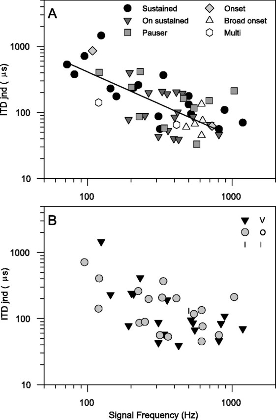
ITD jnds using reference point chosen to yield best jnd. A, Characterized according to PSTH classification type (see Materials and Methods). Line is a power-regression fit to data below 850 Hz. There is one point per unit because PSTHs could be obtained from the data obtained in collecting ITD curves even if no other data were available.B, Characterized according to response area type (see Materials and Methods). Response areas were not always collected because of the premature loss of the unit, so there are fewer points than in A.

The temporal response classification of each unit (Le Beau et al., 1996) is shown using different symbols in Figure 2A. There is an even spread of response types across frequency and ITD jnd, showing, perhaps surprisingly, that the ITD jnd is not influenced by the temporal response type. Similarly, the classification according to response area type (Ramachandran et al., 1999) is also not predictive of ITD jnd (Fig. 2B).

To determine the optimum performance for each unit, we selected the reference ITD to give the lowest ITD jnd, which we call the “best jnd.” However, most psychophysics is done using a midline reference (zero ITD), so it is important to see how using a midline reference affects the ITD jnds. ITD jnds calculated using a midline reference are termed “midline jnds” and are shown by large symbols in Figure3; these are linked by a lineto the corresponding best jnds shown by small dots. The sloping portion of the ITD function is usually centered on midline, so a midline jnd can often be obtained by looking for either an increase or a decrease in firing rate. These jnds may be different, because both the slope of the ITD curve and the variances may be different on either side of the reference ITD. Jnds obtained by looking for either an increase or a decrease in firing rate are equivalent to those obtained choosing thresholds of 75 or 25% correct, respectively, on neurometric curves like those in Figure 1D. Both of these midline jnds were calculated, and the better one is plotted in Figure 3, with jnds obtained by using an increase in firing rate (75% correct) shown by filled symbols and jnds obtained by using a decrease in firing rate (25% correct) shown by open symbols. The midline jnds are larger than the best jnds, which is expected by definition, as shown in Figure 3B comparing the midline jnd on the ordinate against the best jnd on the abscissa. The difference between these jnds can be very large; however, some midline jnds can still be as low as the best jnds, so conclusions about the relationship between human psychophysical performance and neural jnds are unaffected by the choice of reference. It is also interesting that although the midline jnds could occur with either increasing firing rate (toward the peak) or decreasing firing rate (toward the trough) with no a priori reason for choosing one over the other, most of the midline jnds that are shown result from a decrease in firing rate.

Fig. 3.

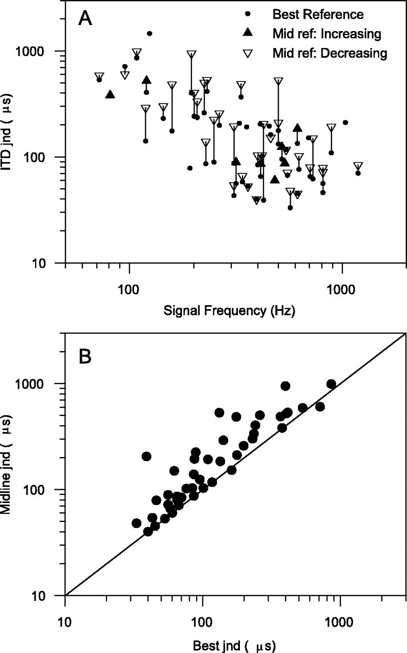
A, ITD jnds using midline reference point (zero ITD). Solid, upward trianglesindicate an increase in firing rate (i.e., 75% correct).Open, downward triangles indicate a decrease in firing rate (i.e., 25% correct). Small,filled circles are ITD jnds using the reference point chosen to yield best jnd, joined to the corresponding midline jnds bylines. B, Comparison of ITD jnds obtained using reference point giving best jnd (abscissa) and those obtained using midline reference point (zero ITD:ordinate). The diagonal line marks equality between jnds.

A comparison of the position of the reference ITD giving rise to the best jnd for increasing firing rate is shown in Figure4 for each unit. Figure4A shows the fine ITD curves for all units plotted over each other after normalizing. The position of the reference point for the best jnd is shown on each curve by a filled circle. Four units had ipsilateral peaks and slope the opposite way from the other curves. Most of the reference points are close to the minimum in the ITD function (just at the “knee-point” where the slope is about to reach its maximum). This results in most of the reference points having ITDs with ipsilateral leading. The positions of the reference points as a function of frequency are shown in Figure4B, with the reference points for curves with ipsilateral peaks shown as open circles. This emphasizes that most of the reference points are at negative ITDs (ipsilateral leading), whereas the peaks of the ITD functions are on the contralateral side (compare Fig. 7C).

Fig. 4.

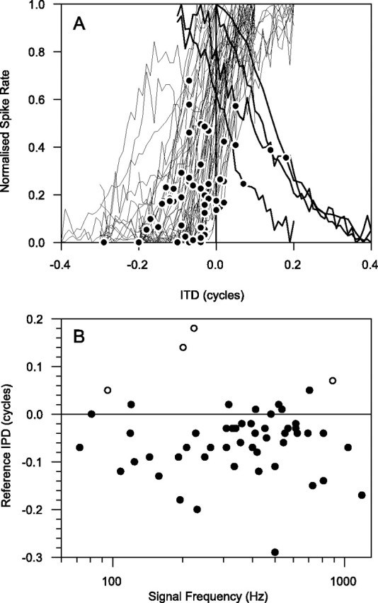
A, Fine ITD curves for all units plotted over each other after normalizing by subtracting off the minimum rate and dividing by the resulting maximum. The position of the reference point for the best jnd is shown on each curve by afilled circle. Four units had ipsilateral peaks and slope the opposite way to the other curves. B, Positions of the reference points. Points from units where the peak of the ITD curve was contralateral are shown as filled circles, and where the peak was ipsilateral they are shown as open circles.

Fig. 7.

A, Comparison of best phase obtained from static tone delay functions (abscissa) and 1 Hz binaural beats (ordinate). B, Comparison of vector strength obtained from static tone delay functions (abscissa) and 1 Hz binaural beats (ordinate). C, Best phase obtained from tone delay curves as a function of signal frequency. The solid line shows the linear regression fit to the data. Thedotted line shows a linear regression fitted to the data obtained from noise delay curves by McAlpine et al. (2001).Symbols indicate PSTH classification; see Figure2A for key.

We investigated the effect of increasing stimulus duration in 16 units, where stability was excellent. This increased the recording time from just under 1 hr to several hours so it was not attempted often. Duration was increased from 50 to 400 msec, and a ratio of on to off duration of 1:3 was maintained; i.e., the longest stimuli were repeated every 1600 msec. The results are shown in Figure5, classified according to the unit temporal response type (Le Beau et al., 1996). Sustained (two of two) (Fig. 5A) and many on-sustained (six of nine) (Fig.5B) units showed an improvement in ITD jnd with increasing signal duration that was less than optimal (log/log slope of −0.5) but comparable with humans (log/log slope of −0.2 shown as dotted line in Fig. 5A). However, some of the on-sustained (three of nine) (Fig. 5B) and all of the pauser (two of two) (Fig. 5C) and broad-onset (three of three) (Fig.5D) units showed poorer ITD jnds as signal duration increased. The decline in performance was caused both by an increase in the variance of spike counts and by a decrease in the peak-to-trough modulation depth of the ITD function; however, we have no clear explanation for why this occurred.

Fig. 5.

ITD jnds as a function of tone duration classified according to PSTH type (see Materials and Methods). A, Sustained units; B, on-sustained units;C, pauser units; D, broad-onset units.Dashed line in A has a slope of −0.2, which corresponds to human psychophysics. Different symbolsindicate different units.

For 19 units we obtained ITD jnds using sound levels of 20 and 40 dB above unit-rate threshold. A comparison of the ITD jnds obtained is shown in Figure 6. In all except three units, the 40 dB jnd is larger than the 20 dB jnd. In human psychophysics (Hershkowitz and Durlach, 1969) the ITD jnd improves significantly up to 20 dB above detection threshold, improves slightly up to 40 dB above detection threshold, and is maintained above that, so these results are slightly surprising. However, they are easily explainable in terms of the rate-level function of the units. Three units had a lower ITD jnd at 40 dB than at 20 dB; these had a monotonically increasing firing rate, which was still increasing between 20 and 40 dB. Of the eight units in which the ITD jnd at 40 dB was >20% greater than the ITD jnd at 20 dB, but still measurable, six had saturated at the best ITD, but the firing rate increased at the worst ITD. In other words, the trough of the ITD function was filling in, and the modulation of the ITD function consequently decreased. The other two units were nonmonotonic, so the peak of the ITD function was reduced, thus reducing the modulation of the ITD function. Of the five units in which the ITD jnd became immeasurably large at 40 dB, four had severely nonmonotonic rate-level functions so that the units did not fire at all at the higher level. The other unit had saturated at the best ITD, but the firing rate increased greatly at the worst ITD, leading to a severely reduced modulation of the ITD function.

Fig. 6.

Comparison of ITD jnds at different signals levels, either 20 dB (▾) or 40 dB (▵) above unit pure-tone rate threshold. For five units, the ITD jnd was too large to be determined at 40 dB, so they are shown at the top of the plot (there are two units at 615 Hz, shown displaced by ±5 Hz).

We determined mean best phase and vector strength from the coarse ITD functions using the method of Goldberg and Brown (1969) by treating the ITD function as a periodic function and converting the ITD to IPD. We also measured the response to binaural beats (at 1 Hz) for many of these neurons and also calculated the mean best phase and vector strength for locking to the beat frequency. The agreement between best phase determined from binaural beats and static tone bursts is shown in Figure 7A and is excellent, with a Pearson correlation coefficient of 0.78. The agreement between vector strengths is less good (Fig. 7B), with a correlation of 0.58. If only the units classified as sustained (15 of 35) or on-sustained (12 of 35) according to the unit temporal response type (Le Beau et al., 1996) were included in the analysis, then the vector strength correlation increased to 0.75 and 0.60, respectively. Units that responded throughout a stimulus, but only after a pause (i.e., pauser types: 5 of 35), gave a lower vector strength correlation of 0.27. Units that responded only at the stimulus onset or offset (onset, broad-onset, and offset types) did not respond sufficiently well to the binaural beat to yield a best phase estimate, so they were not included in the analysis. Since the pioneering work of Yin and Kuwada (Kuwada and Yin, 1983; Yin and Kuwada, 1983a,b; Kuwada et al., 1984), binaural beats have been used routinely to measure ITD sensitivity. These data provide additional confirmation of Yin and Kuwada's findings that this is a valid technique at the level of the IC; however, it does reduce the population of neurons from which binaural best phase can be estimated and has well documented problems with adaptation (Spitzer and Semple, 1993; McAlpine et al., 2000).

Tone best phase tends to increase with frequency (Fig.7C). The linear regression fitted to these data has a slope of 0.109 cycles per kilohertz and an intercept of 0.08 cycles (Fig.7C, solid line). Comparable data derived from noise delay curves were reported by McAlpine et al. (2001); their fit is shown in Figure 7C (dashed line).

Although it might be expected that those units that show the most highly modulated ITD functions would give the lowest ITD jnds, this is not the case. Even when the ITD functions are normalized by subtracting out the baseline rate, there is still no relationship between vector strength and ITD jnd. This is because the jnd is determined primarily by the ratio of the slope of the ITD function to the variance of the firing rate distribution, and the slope of the ITD function is dependent on the stimulus frequency.

Throughout this paper we have shown ITD jnds derived from a ROC analysis. This is computationally more intensive than the alternatives but has the major theoretical advantage of making no assumptions about the underlying spike-rate distributions. The most commonly used measure of discrimination is d′, which assumes that the spike-rate distributions of the target and reference are both Gaussian and have the same variance. Although neither of these assumptions is true,d′ analysis has the major advantage of computational simplicity; only the means and variances of the spike rates need to be computed. In Figure 8 we compare the ITD jnds obtained using both ROC and the standard separation, D, which is a form of d′ in the unequal variance case, obtained by computing the ratio of the difference in mean firing rate divided by the geometric mean of the SDs (Sakitt, 1973; Jiang et al., 1997a). There is a great deal of similarity between the measures (Pearson correlation = 0.986), with the standard separation analysis tending to overestimate the jnds slightly. This similarity is emphasized by the regression line (Fig. 8B,solid line) virtually overlying the line of equality (Fig.8B, dashed line). This suggests that it may be possible to use d′ or the standard separation,D, as a simple way to obtain a quite close approximate estimate of ITD discrimination thresholds of single neurons. To what extent this also applies to stimulus dimensions other then ITD and to sense modalities other than hearing remains to be determined. For this data set, at least, the use of the standard separation, D, would not have significantly biased the results. However, because ROC analysis makes fewer assumptions about the underlying spike-rate distributions, it remains the best method when they are unknown. To used′ (or standard separation) without first testing the spike-rate distributions could introduce biases, so to check that there is no bias the spike-rate distributions for at least a few units would need to be measured and checked for normality.

Fig. 8.

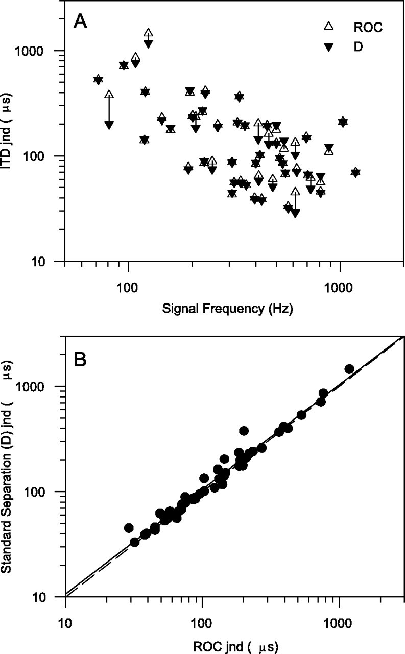
Comparison of ITD jnds obtained from full ROC analysis or by standard separation (D) analysis.A, ITD jnds as a function of signal frequency.B, Scattergram plot of standard separation (D) jnds (ordinate) and ROC jnds (abscissa). Dashed diagonal line marks equality; solid diagonal line is linear regression fit to the data.

Discussion

In a previous paper (Skottun et al., 2001), we showed the basic result illustrated in Figure 2A, without the classification according to PSTH type or response area. We argued that the approach of the lowest jnds to those of human observers was evidence for the sensitivity of single neurons being able to account for human psychophysical jnds. In that paper we discuss the problem of across-species comparison, so we will not pursue that further here. A criticism that could be leveled against that paper is that we compared human psychophysical jnds based on a midline reference with neural jnds based on a reference chosen to give the lowest possible jnd (best jnd). In the current paper, we also compute ITD jnds with a midline reference (Fig. 3A), so a comparison of best jnds (Fig.2A) with midline jnds is possible (Fig.3B). Although for many units midline jnds are higher than the corresponding best jnd, there are many units for which the midline jnds are just as low. The conclusion that single-cell jnds are comparable with human performance still holds.

Fitzpatrick et al. (1997) have argued that the outputs of ∼40 neurons are needed to give discrimination jnds of 16 μsec, on the basis of an analysis of composite ITD curves (which are normally viewed as predictive of noise delay curves). We claim that individual neurons can yield tone discrimination jnds of 30 μsec; however, this does not imply any disagreement about the underlying data but is merely a different way of looking at the results. Fitzpatrick et al. (1997)based their findings on a derivative of the Jeffress delay-line model (Jeffress, 1948) in which they were trying to detect the change in the location of the peak of activity along an ITD ordered line of cells. Instead, we were looking for changes in the firing rate of isolated individual neurons. Looking for shifts in a peak involves looking for a change where the slope of the ITD functions are at their minimum and the variability in the firing rate is at a maximum. This is the least favorable situation for obtaining low jnds, so pooling is required to obtain low jnds. We, on the other hand, were using a method that selected the region of the ITD curve where there was maximal discrimination information. This yielded jnds that were much lower and suggests that single neurons carry enough information to allow discrimination comparable with human psychophysics; however, this does not imply that only a single neuron is used for discrimination. To do so would require previous information about which neuron to use, because in a random field some neurons would show increasing firing rates and some decreasing firing rates in response to the same stimuli. Our results are consistent with the Jeffress delay-line model in which discrimination is performed at the edge of the region of peak activity, a suggestion that has a long history and has been given recent impetus by the findings of McAlpine et al. (2001) followed by Brand et al. (2002), showing that the peaks of ITD functions are often outside the physiological range and the maximal slopes are around midline. Here, the maximal change will be isolated to a few neurons at most, and the identity of the relevant neurons will be signaled by them being at the edge of the distribution. In other words, these results do not prove that single cells are used for ITD discrimination but just that they carry enough information for them to allow this if they can be suitably identified. It should also be noted that the use of an array of several cells with different ITD tunings in concert to perform ITD discrimination is not the same as pooling (which requires the addition of the output of many cells with the same tuning to average out uncorrelated noise). The core finding of this study is that any pooling, or comparison of activity across a population, is performed for reasons other than reducing noise to improve discrimination performance. One possible reason for such a comparison across the population is that there are many factors that can change the firing rate of an individual neuron, such a stimulus level and frequency, as well as stimulus ITD, so a change in firing rate of an individual neuron is ambiguous about what it is signaling. However, a comparison across several cells with similar frequency and level sensitivities would reduce this ambiguity.

The best reference points for increasing firing rates tend to be on the ipsilateral side (Fig. 4). This is despite the fact that peaks of most of the ITD functions are on the contralateral side (Fig.7C). McAlpine et al. (2001) followed by Brand et al. (2002)have argued that there is selective pressure favoring placing the maximum slopes of ITD functions across the midline, so the peaks are pushed into contralateral space and are best-frequency dependent. We also found the same relationship of peak position with best frequency (Fig. 7C). That the best reference points are on the ipsilateral side is consistent with the maximum slope being near midline, because the reference points tended to be slightly toward the minimum of the ITD function relative to the maximum slope (Fig. 4). It is also probably of significance to theories of lateralization discrimination that the better midline jnds were obtained with decreasing spike rates. Cross-correlation-based models of the binaural masking level difference (e.g., Colburn, 1977), supported by physiology (Jiang et al., 1997a,b; Palmer et al., 1999), are also dependent on a decrease in firing rate to indicate the presence of a signal in interaurally in-phase noise.

Although the lowest single unit jnds are in line with human psychophysics, the effects of duration and signal level are not so clear cut. Psychophysical pure tone jnds either remain constant as duration increases (Yost, 1977) or improve slowly with duration with a log–log slope of 0.2 (Ricard and Hafter, 1973; Hafter et al., 1979), which is less than the theoretical optimal improvement assuming independent sampling as a function of duration (a log–log slope of 0.5) (Houtgast and Plomp, 1968). All of the sustained units and many of the on-sustained units showed an improvement comparable with humans (Fig. 5A,B), but all of the other units showed poorer ITD jnds as duration increased. No onset units were tested with a duration sequence for obvious reasons. Thus, to match human psychophysical results, a mechanism for selectively listening to units with a sustained discharge is necessary. To some extent, the units would be self selecting, because the sustained and on-sustained units fire better throughout the stimulus than the other types, but pausers also fire somewhat throughout the longer stimuli, and those on-sustained units that get worse with increasing duration need to be selected out.

The effect of signal level is somewhat more problematic. In human psychophysics (e.g., Hershkowitz and Durlach, 1969), the ITD jnd improves significantly up to 20 dB above detection threshold, improves slightly up to 40 dB above detection threshold, and is maintained above that. Most units, however, show a worsening of ITD jnd between 20 and 40 dB above unit threshold (Fig. 6). Although our results can be explained in terms of the units' rate-level functions, they pose a problem in accounting for the maintenance of the small human psychophysical ITD jnd above 40 dB above detection threshold. Some of the paradox can be explained away by remembering that there is a range of unit rate-level thresholds, so it is possible that some neurons will be within 20 dB of threshold even at the highest levels (75 dB above detection threshold) tested by Hershkowitz and Durlach (1969).

In summary, we have shown that there is sufficient information in the firing rates of individual IC neurons to produce ITD jnds that are comparable with those of humans psychophysically. Although there is enough information, it is unlikely that individual neurons are responsible for the whole animal behavioral response for various reasons, not the least because of the problem of determining which neuron to attend to and the ambiguity inherent in many factors other than ITD affecting the firing rate of an individual neuron. What these results do show is that the common assumption that there must be pooling across cells to allow human psychophysical ITD jnds to be achieved is not true and that any pooling or comparison of activity across a population is performed for reasons other than reducing noise to improve discrimination performance.

References

- 1.Batra R, Kuwada S, Fitzpatrick DC. Sensitivity to interaural temporal disparities of low- and high-frequency neurons in the superior olivary complex. I. Heterogeneity of responses. J Neurophysiol. 1997a;73:1222–1236. doi: 10.1152/jn.1997.78.3.1222. [DOI] [PubMed] [Google Scholar]
- 2.Batra R, Kuwada S, Fitzpatrick DC. Sensitivity to interaural temporal disparitites of low- and high-frequency neurons in the superior olivary complex. II. Coincidence detection. J Neurophysiol. 1997b;78:1237–1247. doi: 10.1152/jn.1997.78.3.1237. [DOI] [PubMed] [Google Scholar]
- 3.Bradley A, Skottun BC, Ohzawa I, Sclar G, Freeman RD. A neurophysiological evaluation of the differential response model for orientation and spatial-frequency discrimination. J Opt Soc Am [A] 1985;2:1607–1610. doi: 10.1364/josaa.2.001607. [DOI] [PubMed] [Google Scholar]
- 4.Bradley A, Skottun BC, Ohzawa I, Sclar G, Freeman RD. Visual orientation and spatial frequency discrimination: a comparison of single neurons and behavior. J Neurophysiol. 1987;57:755–772. doi: 10.1152/jn.1987.57.3.755. [DOI] [PubMed] [Google Scholar]
- 5.Brand A, Behrend O, Marquardt T, McAlpine D, Grothe B. Precise inhibition is essential for microsecond interaural time difference coding. Nature. 2002;417:543–547. doi: 10.1038/417543a. [DOI] [PubMed] [Google Scholar]
- 6.Bullock DC, Palmer AR, Rees A. Compact and easy-to-use tungsten-in-glass microelectrode manufacturing workstation. Med Biol Eng Comput. 1988;26:669–672. doi: 10.1007/BF02447511. [DOI] [PubMed] [Google Scholar]
- 7.Carr CE. Processing of temporal information in the brain. Annu Rev Neurosci. 1993;16:223–243. doi: 10.1146/annurev.ne.16.030193.001255. [DOI] [PubMed] [Google Scholar]
- 8.Cohn TE, Green DG, Tanner WP. Receiver operating characteristic analysis. Application to the study of quantum fluctuation effects in optic nerve of rana pipiens. J Gen Physiol. 1975;66:583–616. doi: 10.1085/jgp.66.5.583. [DOI] [PMC free article] [PubMed] [Google Scholar]
- 9.Colburn HS. Theory of binaural interaction based on auditory-nerve data. II. Detection of tones in noise. J Acoust Soc Am. 1977;61:525–533. doi: 10.1121/1.381294. [DOI] [PubMed] [Google Scholar]
- 10.Durlach NI, Colburn HS. Binaural phenomena. In: Carterette EC, Friedman MP, editors. Handbook of perception, Vol IV, hearing. Academic; New York: 1978. pp. 365–466. [Google Scholar]
- 11.Fay RR, Coombs SL. Psychometric functions for level discrimination and the effects of signal duration in the goldfish (carassius-auratus)—psychophysics and neurophysiology. J Acoust Soc Am. 1992;92:189–201. doi: 10.1121/1.404282. [DOI] [PubMed] [Google Scholar]
- 12.Fitzpatrick DC, Batra R, Stanford TR, Kuwada S. A neuronal population code for sound localization. Nature. 1997;388:871–874. doi: 10.1038/42246. [DOI] [PubMed] [Google Scholar]
- 13.Gerstner W, Kempter R, van Hemmen JL, Wagner H. A neuronal learning rule for sub-millisecond temporal coding. Nature. 1996;383:76–78. doi: 10.1038/383076a0. [DOI] [PubMed] [Google Scholar]
- 14.Goldberg JM, Brown PB. Response of binaural neurons of dog superior olivary complex to dichotic tonal stimuli: some physiological mechanisms of sound localization. J Neurophysiol. 1969;32:613–636. doi: 10.1152/jn.1969.32.4.613. [DOI] [PubMed] [Google Scholar]
- 15.Green DM, Swets JA. Signal detection theory and psychophysics. Krieger; Huntington, NY: 1974. [Google Scholar]
- 16.Hafter ER, Dye RH, Gilkey RH. Lateralization of tonal signals which have neither onsets nor offsets. J Acoust Soc Am. 1979;65:471–477. doi: 10.1121/1.382346. [DOI] [PubMed] [Google Scholar]
- 17.Hall JL. Binaural interaction in the acessory superior-olivary nucleus of the cat. J Acoust Soc Am. 1965;37:814–823. doi: 10.1121/1.1909447. [DOI] [PubMed] [Google Scholar]
- 18.Hawken MJ, Parker AJ. Detection and discrimination mechanisms in the striate cortex of the old-world monkey. In: Blakemore C, editor. Vision: Coding and efficiency. Cambridge UP; Cambridge, UK: 1990. pp. 103–116. [Google Scholar]
- 19.Hershkowitz RM, Durlach NI. Interaural time and amplitude jnds for a 500-Hz tone. J Acoust Soc Am. 1969;46:1464–1467. doi: 10.1121/1.1911887. [DOI] [PubMed] [Google Scholar]
- 20.Houtgast T, Plomp R. Lateralization threshold of a signal in noise. J Acoust Soc Am. 1968;44:807–812. doi: 10.1121/1.1911178. [DOI] [PubMed] [Google Scholar]
- 21.Jeffress LA. A place theory of sound localization. J Comp Psychol. 1948;44:35–39. doi: 10.1037/h0061495. [DOI] [PubMed] [Google Scholar]
- 22.Jiang D, McAlpine D, Palmer AR. Detectability index measures of binaural masking level difference across populations of inferior colliculus neurons. J Neurosci. 1997a;17:9331–9339. doi: 10.1523/JNEUROSCI.17-23-09331.1997. [DOI] [PMC free article] [PubMed] [Google Scholar]
- 23.Jiang D, McAlpine D, Palmer AR. Responses of neurones in the guinea pig inferior colliculus to binaural masking level difference stimuli measured by rate-versus-level functions. J Neurophysiol. 1997b;77:3085–3106. doi: 10.1152/jn.1997.77.6.3085. [DOI] [PubMed] [Google Scholar]
- 24.Johansson RS, Vallbo ÅB. Detection of tactile stimuli. Thresholds of afferent units related to psychophysical thresholds in the human hand. J Physiol (Lond) 1979;297:405–422. doi: 10.1113/jphysiol.1979.sp013048. [DOI] [PMC free article] [PubMed] [Google Scholar]
- 25.Kuwada S, Yin TCT. Binaural interaction in low-frequency neurons in inferior colliculus of the cat. I. Effects of long interaural delays, intensity, and repetition rate on interaural delay function. J Neurophysiol. 1983;50:981–999. doi: 10.1152/jn.1983.50.4.981. [DOI] [PubMed] [Google Scholar]
- 26.Kuwada S, Yin TCT, Syka J, Buunen TJF, Wickesberg RE. Binaural interaction in low-frequency neurons in inferior colliculus of the cat. IV. Comparison of monaural and binaural response properties. J Neurophysiol. 1984;51:1306–1325. doi: 10.1152/jn.1984.51.6.1306. [DOI] [PubMed] [Google Scholar]
- 27.Le Beau FEN, Rees A, Malmierca MS. Contribution of GABA- and glycine-mediated inhibition to the monaural temporal response properties of neurons in the inferior colliculus. J Neurophysiol. 1996;75:902–919. doi: 10.1152/jn.1996.75.2.902. [DOI] [PubMed] [Google Scholar]
- 28.McAlpine D, Jiang D, Shackleton TM, Palmer AR. Convergent input from brainstem coincidence detectors onto delay-sensitive neurons in the inferior colliculus. J Neurosci. 1998;18:6026–6039. doi: 10.1523/JNEUROSCI.18-15-06026.1998. [DOI] [PMC free article] [PubMed] [Google Scholar]
- 29.McAlpine D, Jiang D, Shackleton TM, Palmer AR. Responses of neurons in the inferior colliculus to dynamic interaural phase cues: evidence for a mechanism of binaural adaptation. J Neurophysiol. 2000;83:1356–1365. doi: 10.1152/jn.2000.83.3.1356. [DOI] [PubMed] [Google Scholar]
- 30.McAlpine D, Jiang D, Palmer AR. A neural code for low-frequency sound localisation in mammals. Nat Neurosci. 2001;4:396–401. doi: 10.1038/86049. [DOI] [PubMed] [Google Scholar]
- 31.Mills AW. On the minimum audible angle. J Acoust Soc Am. 1958;30:237–246. [Google Scholar]
- 32.Newsome WT, Britten KH, Movshon JA. Neuronal correlates of a perceptual decision. Nature. 1989;341:52–54. doi: 10.1038/341052a0. [DOI] [PubMed] [Google Scholar]
- 33.Palmer AR, Jiang D, McAlpine D. Desynchronizing responses to correlated noise: a mechanism for binaural masking levels differences at the inferior colliculus. J Neurophysiol. 1999;81:722–734. doi: 10.1152/jn.1999.81.2.722. [DOI] [PubMed] [Google Scholar]
- 34.Parker AJ, Hawken MJ. Capabilities of monkey cortical cells in spatial-resolution tasks. J Opt Soc Am [A] 1985;2:1101–1114. doi: 10.1364/josaa.2.001101. [DOI] [PubMed] [Google Scholar]
- 35.Ramachandran R, Davis KA, May BJ. Single-unit responses in the inferior colliculus of decerebrate cats I. Classification based on frequency response maps. J Neurophysiol. 1999;82:152–163. doi: 10.1152/jn.1999.82.1.152. [DOI] [PubMed] [Google Scholar]
- 36.Relkin EM, Pelli DG. Probe tone thresholds in the auditory nerve measured by two-interval forced-choice procedures. J Acoust Soc Am. 1987;82:1679–1691. doi: 10.1121/1.395159. [DOI] [PubMed] [Google Scholar]
- 37.Relkin EM, Turner CW. A reexamination of forward masking in the auditory nerve. J Acoust Soc Am. 1988;84:584–591. doi: 10.1121/1.396836. [DOI] [PubMed] [Google Scholar]
- 38.Ricard GC, Hafter ER. Detection of interaural time differences in short duration, low frequency tones. J Acoust Soc Am. 1973;53:335. [Google Scholar]
- 39.Sakitt B. Indices of discriminability. Nature. 1973;241:133–134. doi: 10.1038/241133a0. [DOI] [PubMed] [Google Scholar]
- 40.Skottun BC. Sound localization and neurons. Nature. 1998;393:531. doi: 10.1038/31134. [DOI] [PubMed] [Google Scholar]
- 41.Skottun BC, Shackleton TM, Arnott RH, Palmer AR. The ability of inferior colliculus neurons to signal differences in interaural delay. Proc Natl Acad Sci USA. 2001;98:14050–14054. doi: 10.1073/pnas.241513998. [DOI] [PMC free article] [PubMed] [Google Scholar]
- 42.Spitzer MW, Semple MN. Responses of inferior colliculus neurones to time-varying interaural phase disparity: effects of shifting the locus of virtual motion. J Neurophysiol. 1993;69:1245–1263. doi: 10.1152/jn.1993.69.4.1245. [DOI] [PubMed] [Google Scholar]
- 43.Spitzer MW, Semple MN. Neurons sensitive to interaural phase disparity in gerbil superior olive: diverse monaural and temporal response properties. J Neurophysiol. 1995;73:1668–1690. doi: 10.1152/jn.1995.73.4.1668. [DOI] [PubMed] [Google Scholar]
- 44.Stanford TR, Kuwada S, Batra R. A comparison of the interaural time sensitivity of neurons in the inferior colliculus and thalamus of the unanesthetized rabbit. J Neurosci. 1992;12:3200–3216. doi: 10.1523/JNEUROSCI.12-08-03200.1992. [DOI] [PMC free article] [PubMed] [Google Scholar]
- 45.Vallbo ÅB. Single-afferent neurons and somatic sensation in humans. In: Gazzaniga MS, editor. The cognitive neurosciences. MIT; Cambridge, MA: 1995. pp. 237–252. [Google Scholar]
- 46.Yin TCT, Chan JCK. Neural mechanisms underlying interaural time sensitivity to tones and noise. In: Edelman GM, Gall WE, Cowan WM, editors. Auditory function: neurobiological bases of hearing. Wiley; New York: 1988. pp. 385–430. [Google Scholar]
- 47.Yin TCT, Chan JCK. Interaural time sensitivity in medial superior olive of cat. J Neurophysiol. 1990;64:465–488. doi: 10.1152/jn.1990.64.2.465. [DOI] [PubMed] [Google Scholar]
- 48.Yin TCT, Kuwada S. Binaural interaction in low-frequency neurons in inferior colliculus of the cat. II. Effects of changing rate and direction of interaural phase. J Neurophysiol. 1983a;50:1000–1019. doi: 10.1152/jn.1983.50.4.1000. [DOI] [PubMed] [Google Scholar]
- 49.Yin TCT, Kuwada S. Binaural interaction in low-frequency neurons in inferior colliculus of the cat. III. Effects of changing frequency. J Neurophysiol. 1983b;50:1020–1042. doi: 10.1152/jn.1983.50.4.1020. [DOI] [PubMed] [Google Scholar]
- 50.Yin TCT, Joris PX, Smith PH, Chan JCK. Neuronal processing for coding interaural time disparities. In: Gilkey RH, Anderson TR, editors. Binaural and spatial hearing in real and virtual environments. Erlbaum; Mahwah, NJ: 1997. pp. 427–445. [Google Scholar]
- 51.Yost WA. Lateralization of pulsed sinusoids based on interaural onset, ongoing, and offset temporal differences. J Acoust Soc Am. 1977;61:190–194. doi: 10.1121/1.381254. [DOI] [PubMed] [Google Scholar]
- 52.Young ED, Barta PE. Rate responses of auditory nerve fibers to tones in noise near masked threshold. J Acoust Soc Am. 1986;79:426–442. doi: 10.1121/1.393530. [DOI] [PubMed] [Google Scholar]