Structured light imaging for breast-conserving surgery, part II: texture analysis and classification

Abstract.

Subdiffuse spatial frequency domain imaging (sd-SFDI) data of 42 freshly excised, bread-loafed tumor resections from breast-conserving surgery (BCS) were evaluated using texture analysis and a machine learning framework for tissue classification. Resections contained 56 regions of interest (RoIs) determined by expert histopathological analysis. RoIs were coregistered with sd-SFDI data and sampled into $\sim 4\times 4{\mathrm{mm}}^2$ subimage samples of confirmed and homogeneous histological categories. Sd-SFDI reflectance textures were analyzed using gray-level co-occurrence matrix pixel statistics, image primitives, and power spectral density curve parameters. Texture metrics exhibited statistical significance ($p\text{-value}<0.05$) between three benign and three malignant tissue subtypes. Pairs of benign and malignant subtypes underwent texture-based, binary classification with correlation-based feature selection. Classification performance was evaluated using fivefold cross-validation and feature grid searching. Classification using subdiffuse, monochromatic reflectance (illumination spatial frequency of $f_x=1.37{\mathrm{mm}}^{-1}$, optical wavelength of $\lambda =490\mathrm{nm}$) achieved accuracies ranging from 0.55 (95% CI: 0.41 to 0.69) to 0.95 (95% CI: 0.90 to 1.00) depending on the benign–malignant diagnosis pair. Texture analysis of sd-SFDI data maintains the spatial context within images, is free of light transport model assumptions, and may provide an alternative, computationally efficient approach for wide field-of-view (${\mathrm{cm}}^2$) BCS tumor margin assessment relative to pixel-based optical scatter or color properties alone.

1. Introduction

Breast-conserving surgery (BCS) in combination with radiation therapy is the most common treatment for stage I and II breast cancer.^1,2 For BCS to be effective, excised tissue margins must be clear of malignancy (i.e., negative margins). However, 15% to 35% of BCS patients require a second surgery due to incomplete initial excision (i.e., one or more positive margins) as determined by histopathological analysis.^3–8 Identification of cancer at the margin is a spatial detection problem, filtered visually by pathology technicians and pathologists performing labor-intensive searches of tissue sections. Several techniques have been proposed for improved BCS margin assessment, but significant limitations associated with each approach have prevented their widespread adoption.⁷ Common techniques include electrical impedance;^9,10 diffuse reflectance¹¹ and Raman spectroscopic point-sampling;¹² touch-prep cytology;¹³ and frozen section pathology.¹⁴ Importantly, point-sampling methods lack a comprehensive and/or practical approach to wide field-of-view (FOV) detection and thus are inherently time-consuming. Touch-prep cytology and frozen section pathology are resource-intensive to process even a subsection of a BCS specimen and suffer slow turnaround times.¹³ Most techniques lack the speed and wide FOV required to intraoperatively interrogate an entire BCS lump.

Technology assessment studies often adopt broad tissue categories, such as normal versus malignant.⁷ This categorization lumps together healthy adipose and fibroglandular tissues with benign lesions, such as fibrocystic disease (FCD), although these tissue subtypes contain different cellular and subcellular structures. Malignant tissue subtypes, including invasive ductal carcinoma (IDC) of low, intermediate, and high grade and invasive lobular carcinoma (ILC), are all characterized by different densities of nuclei and mitochondria, and different types and organizations of cells. Nevertheless, these malignant tissue subtypes are also commonly lumped together into a single malignant tissue category. Studies that rely on broad tissue categorization complicate the tissue classification task and jeopardize clinical potential. The problem of intraoperative breast tissue classification could be simplified by ensuring sensitivity to key benign and malignant breast tissue subtypes. In addition, biopsies are performed prior to BCS procedures, and using this a priori tissue information could improve tissue margin diagnostic accuracy by reducing the number of possible malignant tissue subtypes.¹⁵

Wide FOV (${10}^0-{10}^2{\mathrm{cm}}^2$) structured light imaging, also known as spatial frequency-domain imaging (SFDI), involves illuminating tissue samples with one-dimensional (1-D) sinusoidal patterns at different spatial frequencies ($f_x$) and optical wavelengths ($\lambda$). Using a diffuse or subdiffuse light transport model, SFDI data can determine the optical absorption and scattering properties of biological tissue.^16,17 A strength of SFDI is that it can be readily implemented with standard imaging and display hardware. Perhaps most promisingly in the context of surface tissue characterization (e.g., BCS margin assessment), the illumination pattern $f_x$ and $\lambda$ can be honed to decrease sensitivity to absorption, increase sensitivity to scatter, and enhance contrast to surface tissue ultrastructures. This is accomplished by using high spatial frequencies¹⁸ and relatively short optical wavelengths.¹⁹ The combination reduces photon density wave penetration depth, avoids volumetric averaging over tortuous photon pathlengths, and thereby natively enhances spatial resolution. At sufficiently high spatial frequencies, SFDI illumination penetrates to depths less than the length scale of diffuse photon propagation. Photons are intrinsically confined to surface tissue and are most sensitive to large, single backscattering events with the angle and intensity of reflectance dependent on cellular ultrastructures.²⁰ In this regime, the modality is termed high spatial frequency (HSF) structured light imaging^15,21 or subdiffuse SFDI (sd-SFDI).²²

Previous studies have investigated diffuse and subdiffuse SFDI for BCS specimen margin assessment using optical properties.^22–24 The work presented here represents part II of a two-part paper and used the largest SFDI dataset of fresh BCS tissue specimens published to date with the most extensive categorization of benign and malignant tissue subtypes. The complete dataset was introduced in part I of this paper,¹⁵ which focused on optical scatter and color property quantification. Optical scatter and color properties have demonstrated potential for breast tumor margin assessment. However, both types of properties are inherently pixel-based, lacking spatial context between pixels.¹⁵ Furthermore, optical property quantification necessitates significant computation, requiring either nonlinear least squares fitting of data to an appropriate light transport model or the generation of an empirical look-up table using a Monte Carlo model.^16,25 The process can be slow,²² and model-based inversion fitting can introduce additional errors.¹⁶

Texture analysis refers to the appearance, structure, and arrangement of features within an image and thus inherently relies on the spatial relationship of multiple pixels in an image. Here, in part II, the SFDI dataset introduced in part I was reprocessed using texture analysis and a machine learning framework for tissue subtype classification. The primary objectives of part II are twofold. First, the authors introduce an sd-SFDI imaging and analysis protocol for BCS tissue surface characterization that uses one spatial frequency ($f_x=1.37{\mathrm{mm}}^{-1}$), one optical wavelength ($\lambda =490\mathrm{nm}$), and reflectance texture instead of tissue optical and/or color properties. The protocol leverages subdiffuse scatter as a contrast mechanism. It benefits from a relatively fast acquisition time and increased computational efficiency, because property quantification does not involve inverse model fitting. Importantly, the protocol avoids light transport model assumptions for metric quantitation. Second, the statistical significance of a limited set of statistical, structural, and transform-based texture metrics is evaluated by hypothesis testing, and the relative importance of these metrics is evaluated by a classification model.

2. Materials and Methods

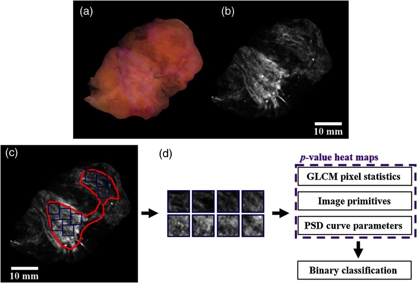
Details regarding the imaging system are given in Sec. 2.1. The clinical study protocol for this paper is outlined in Sec. 2.2. Figure 1 shows the processing workflow for part II of this paper: region of interest (RoI) sampling, texture metric quantitation and statistical analysis, and classification. These steps are discussed in detail in Secs. 2.3, 2.4, and 2.5, respectively.

Fig. 1.

The processing workflow for this paper: (a) RGB color space, diffuse illumination ($f_x=0.00{\mathrm{mm}}^{-1}$) “naked eye” reconstruction according to Ref. 21 for comparison; (b) subdiffuse reflectance ($f_x=1.37{\mathrm{mm}}^{-1}$), monochromatic ($\lambda =490\mathrm{nm}$) image of the same specimen; (c) specimen with ILC lesion RoI (red) and sampled subimages (blue); and (d) subimage texture analysis, statistical analysis, and classification.

2.1. Instrumentation

A multimodal imaging system that combines SFDI and microcomputed tomography imaged all BCS tissue specimens in this study. The experimental performance of the system was determined previously.²¹ The highest spatial resolution demonstrated by the SFDI subsystem was $3.78\text{\hspace{0.17em}\hspace{0.17em}cycles}/\mathrm{mm}$ and involved using the highest spatial frequency possible ($f_x=1.37{\mathrm{mm}}^{-1}$) and lowest optical wavelength at which data were collected ($\lambda =490\mathrm{nm}$). This specific spatial frequency was the highest achievable experimentally, given the SFDI subsystem geometry and the limitations of the digital micromirror device used.²¹ Each specimen was placed between two custom laser-cut, optically clear acrylic plates and secured using elastic bands. Fixing the specimen in the holder provided a flat imaging surface. The projector, stage, and camera created an off-axis projection scheme. The flat imaging surface and off-axis projection reduced the occurrence of specular reflections.²¹ Crossed polarizers were not used in this case to avoid undesired rejection of subdiffusely scattered photons, which undergo a phase shift close to 180 deg. Data acquisition followed the standard SFDI procedure of imaging at three phase offsets (i.e., ${\mathrm{\Phi }}_1=0\mathrm{deg}$, ${\mathrm{\Phi }}_2=120\mathrm{deg}$, ${\mathrm{\Phi }}_3=240\mathrm{deg}$) then combining the three phases using pixel-by-pixel demodulation for a given $f_x$ and $\lambda$ pair.²⁶ Demodulated reflectance data were normalized and median filtered using a $3\times 3\text{-pixel}$ kernel prior to further processing.

2.2. Study Protocol

Imaging was performed at the Dartmouth Hitchcock Medical Center (DHMC) in Lebanon, New Hampshire. The clinical study was approved by the Institutional Review Board at Dartmouth College and DHMC for the protection of human subjects, and all procedures followed the approved protocol. Procurement of tissue specimens involved patients undergoing consented and elective breast surgeries at DHMC.

Specimen imaging occurred postoperatively during standard pathological processing and did not hinder clinical workflow. A resected tumor was “bread-loafed” or sliced into $\sim 5\text{-}\mathrm{mm}$ sections along the axis perpendicular to the long axis of the lump. One slice from the lump was selected by a pathology specialist and imaged with random anatomical orientation. Image data were therefore assumed to be free of rotational bias. After standard-of-care histological processing and staining with hematoxylin and eosin, a board-certified breast pathologist (Wells) determined microscopic RoIs that were manually coregistered to wide FOV SFDI data. For an imaged slice, SFDI RoIs were conservatively outlined within the histopathologic RoIs. RoIs did not necessarily encompass the entirety of each specimen. Many lesions were relatively small compared to the total surface area of the specimens. RoI selection was intentionally conservative to ensure that the regions were completely contained within the lesions.

A summary of all enrolled tissues can be found in part I of this paper.¹⁵ For the texture analysis here, the enrolled tissue RoIs were sampled to create square subimages of constant size. The sampling process resulted in a subset of the original dataset being considered for texture analysis.

2.3. Region of Interest Sampling

Texture analysis was performed on $32\times 32\text{-pixel}$ (i.e., $\sim 4\times 4{\mathrm{mm}}^2$) subimage samples extracted from each specimen RoI. The size was chosen such that macroscale tissue features were captured in each subimage. Square subimage sampling enabled direct comparisons of localized tissue textures found in different tissue subtypes. A custom MATLAB script implemented a simple sliding-box algorithm for subimage sampling, which is demonstrated in Figs. 1(c) and 1(d). Tissue diagnoses found in fewer than $n=3$ specimens and RoIs too small to contain a single sample were excluded. Samples with large specular reflections were identified and censured via a custom MATLAB script based on the median absolute deviation of pixel intensities in each sample. A total of 42 specimens containing 56 RoIs (37 benign and 19 malignant) met these criteria. The primary cause for data exclusion was the requirement of a $\sim 4\times 4{\mathrm{mm}}^2$ sample of confirmed and homogeneous tissue. Several lesion RoIs in the dataset were too small or irregular in shape to contain a $\sim 4\times 4{\mathrm{mm}}^2$ sample. The 56 eligible RoIs provided a total of 163 subimages (100 benign and 63 malignant) for texture analysis. Table 1 summarizes the 163 samples with respect to tissue subtype, specimen (or RoI) count, and sample count.

Table 1.

Summary of $32\times 32\text{-pixel}$ ($\sim 4\times 4{\mathrm{mm}}^2$) SFDI reflectance samples with benign diagnoses in bold and malignant diagnoses in italic.

Tissue subtype	Specimen (RoI) count	Sample count
Adipose	26	56
Connective	6	20
FCD	5	24
Intermediate-grade IDC	5	14
High-grade IDC	8	29
ILC	6	20
Total	56	163

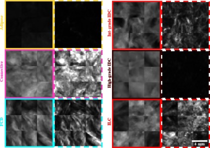
Benign tissue subtypes considered for texture analysis were adipose tissue, connective tissue, and FCD. Fibroadenoma was not included in the analysis. This type of benign lesion, although present in sufficient numbers for inclusion (4 RoIs and 24 samples), was assumed to be of nominal clinical importance, because it is typically known prior to surgery and rarely warrants a re-excision procedure.²⁷ Malignant subtypes considered for texture analysis were intermediate- and high-grade IDC and ILC (i.e., only invasive cancers). Representative samples from the six tissue subtypes are shown in Fig. 2. In the figure, the bordering around each $3\times 3$ block of samples is color-coded by tissue subtype. The solid border denotes diffuse, planar illumination reflectance ($f_x=0.00{\mathrm{mm}}^{-1}$, $\lambda =490\mathrm{nm}$) derived from the SFDI data. The dashed border denotes subdiffuse reflectance ($f_x=1.37{\mathrm{mm}}^{-1}$, $\lambda =490\mathrm{nm}$) derived from the SFDI data. The same tissue samples are displayed in the diffuse and subdiffuse reflectance panes. The comparison demonstrates that subdiffuse reflectance is sensitive to small-scale surface tissue features that are occult to typical, planar illumination imaging. Furthermore, the figure shows how sd-SFDI scatter might function as a useful surface tissue contrast mechanism. Section 3.1 relates the various subdiffuse reflectance textures observed in Fig. 2 to underlying tissue subtype compositions.

Fig. 2.

Representative samples of the normal and benign tissues (left column) and malignant tissues (right column). Panes are color-coded by tissue subtype. Solid boarders denote planar, diffuse illumination ($f_x=0.00{\mathrm{mm}}^{-1}$, $\lambda =490\mathrm{nm}$) reflectance. Dashed boarders denote subdiffuse illumination ($f_x=1.37{\mathrm{mm}}^{-1}$, $\lambda =490\mathrm{nm}$) reflectance. Scalebar is shown in the bottom-right corner.

2.4. Texture Analysis

Texture analysis of spectroscopic images is known to provide unique information about scattering ultrastructures in human breast tissues.²⁷ Here, texture is considered an analysis tool for sd-SFDI data. A variety of texture representations were explored in this paper, all of which can be broadly categorized as statistical, structural, or transform-based in nature. These three representations of texture have been used to analyze radiological images of biological tissues, including mammography.²⁸ Statistical metrics included gray-level co-occurrence matrix (GLCM) contrast, correlation, and homogeneity.²⁷ Structural or image primitive metrics included fractal dimension, lacunarity, and Euler number.^27,29–31 Transform-based metrics were derived from Fourier transform power spectral density (PSD) curve linear fit parameters.³² Details associated with GLCM pixel statistics, structural image primitives, and Fourier transform PSD curve parameters are given in Secs. 2.4.1, 2.4.2, and 2.4.3, respectively.

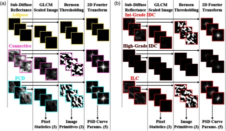
Texture analysis generated a total of eleven features associated with each sample. Table 2 summarizes the number of metrics associated with each representation of texture. All metrics were quantified rapidly for each sample ($<1\mathrm{s}$). Figure 3 provides an overview of the three representations of texture investigated here and gives qualitative comparisons between tissue subtypes undergoing each type of texture analysis.

Table 2.

Summary of texture metrics quantified for each sample.

Texture analysis method	Metric count
Pixel statistics	3
Image primitives	3
PSD curve parameterization	5
Total	11

Fig. 3.

Overview of the three texture analysis approaches in this paper: GLCM pixel statistics, structural image primitives, and Fourier transform PSD curve parameters. Flow of processing starts with sampled reflectance samples, which are converted to binary images via Bernsen thresholding, to GLCM scaled images, and to the frequency domain via a 2-D Fourier transform for metric quantification. Representative subimage samples are shown for (a) normal and benign tissue subtypes and (b) malignant tissue subtypes. Dashed arrows signify additional processing steps.

The Mann-Whitney U-test is used to test the null hypothesis that two samples come from the same population. The Mann-Whitney U-test was chosen to quantify p-values due to small sample sizes and to avoid the assumption of normally distributed metrics. U-test $p$-values quantified the statistical significance of pixel statistics, image primitives, and PSD curve parameters between the three benign and three malignant tissue subtypes.

2.4.1. Gray-level co-occurrence matrix pixel statistics

The GLCM representation of texture features assesses the spatial dependence of pixel intensities within an image. Pixel statistics of contrast, correlation, and homogeneity were calculated for each sample based on eight-level grayscale intensity images ($8\times 8$-element GLCMs). Contrast quantifies the local variation in an image, correlation measures its gray-tone linear dependencies, and homogeneity assesses the prevalence of gray-tone transitions.³³ Each GLCM invoked a one-pixel displacement distance and vector directionality symmetric about 0 deg, 45 deg, 90 deg, and 135 deg. Reported values were averaged over the four angles. Each GLCM was generated using the MATLAB graycomatrix function, and statistics were quantified via the MATLAB graycoprops function.³⁴

2.4.2. Image primitives

The arrangement of repeating patterns or features in an image, referred to as image primitives, were also used to characterize texture. Samples were converted into binary format using a Bernsen local thresholding algorithm implemented in MATLAB.^35,36 Bernsen thresholding is based on local contrast within a moving window (a $13\times 13\text{-pixel}$ window here). Local contrast thresholding was found to effectively isolate reflectance structures sometimes lost by global thresholding. Euler number, fractal dimension, and lacunarity were quantified for each binary sample. Euler number codifies the difference between the number of connected components or objects in an image and the number of holes in those objects. Euler number was computed using the MATLAB function bweuler.³⁴ The Hausdorff box-counting fractal dimension, which is a measure of self-similarity and roughness in an image, was computed using the MATLAB function hausDim.^37,38 Lacunarity is a measure of inhomogeneity or transitional and rotational invariance of features in an image. Lacunarity was computed by the MATLAB function lacunarity_glbox.³⁹

2.4.3. Power spectral density curve parameters

A PSD curve depicts the relative amplitude of spatial frequencies within an image. The PSD curve of each sample was calculated via a two-dimensional (2-D) discrete Fourier transform followed by radial averaging of the amplitude of the shifted image data. Radial averaging decomposed the 2-D image into a 1-D profile, which was then converted to power and normalized by its maximum value. Normalized PSD curves were derived using an adapted form of the MATLAB function raPsd2d.⁴⁰ Parameterization involved visual identification of two distinct spatial frequency ranges that consistently exhibited different slopes in the PSD curves. These two spatial frequency ranges formed low spatial frequency (LSF) and HSF PSD contributions. Linear fits were applied to these two spatial frequency ranges, yielding slope and intercept parameters for each contribution. The spatial frequency at which the two linear fits intersected provided a fifth parameter.

The LSF and HSF ranges for linear fit parameterization were set to 0 to $1{\mathrm{mm}}^{-1}$ and 1 to $2{\mathrm{mm}}^{-1}$, respectively. These ranges were selected after inspection of an ensemble of PSD curves for all samples, shown in Fig. 4(a). In Fig. 4(b), the five linear fit parameters derived from each PSD curve are illustrated. To demonstrate the potential value of PSD curve parameterization, the PSD curves for all adipose tissue and ILC samples tallied in Table 1 are plotted together in Fig. 4(b). Adipose tissue and ILC samples contain significantly different spatial frequency content indicated by different HSF linear fit slopes and intercepts. In contrast, visual inspection of all FCD and ILC PSD curves, plotted together in Fig. 4(c), shows similar linear fits. The comparison in Figs. 4(b) and 4(c) reinforces the concept that different representations of texture may be effective at distinguishing different types of tissue. With reference to Fig. 2, the comparison also highlights the fact that when tissues appear different visually, texture-based feature extraction algorithms are likely to discriminate them quantitatively.

Fig. 4.

Normalized PSD curves for (a) all $f_x=1.37{\mathrm{mm}}^{-1}$, $\lambda =490\mathrm{nm}$ samples tallied in Table 1; (b) only adipose and ILC samples with linear fits applied to each diagnosis separately; and (c) only FCD and ILC samples with linear fits applied to each diagnosis separately. Vertical, dashed, black and blue lines delimit the LSF and HSF linear fit ranges, respectively. The derivation of the five PSD linear fit parameters is illustrated in (b) in green.

2.5. Classification Analysis

Previous studies have combined SFDI with classification analysis. Laughney et al.²³ were the first to apply SFDI to breast cancer pathology discrimination. They used SFDI-derived optical properties and a nearest-neighbor learning algorithm to discriminate normal, fibroadenoma, ductal carcinoma in situ, invasive cancer, and treated invasive cancer tissues with 82% accuracy. McClatchy et al. used SFDI-derived optical properties to predict stromal, epithelial, and adipose fractions in surgically resected breast tissues with a threshold-based tissue classification model. They demonstrated pixel-level classification accuracy of 75% and specimen-level accuracy of 84%.²⁴ Beyond breast tissue characterization, recent work by Rowland et al.⁴¹ used SFDI reflectance data at multiple spatial frequencies to predict burn severity in a porcine model using a cubic support vector machine (SVM) classifier. At 24 h, they demonstrated 92.5% accuracy classifying burn severity.

In this work, sd-SFDI reflectance texture metrics were provided as input to a machine learning framework for tissue subtype classification. Binary classifications were performed between the three benign and three malignant breast tissue diagnoses. Texture feature vectors (11 total features, detailed in Table 2) associated with one benign tissue subtype and one malignant tissue subtype were classified using a linear SVM classifier (MATLAB function fitcsvm with default settings⁴²) with correlation-based feature selection. Classification performance was evaluated using random fivefold cross-validation (CV). Fivefold CV was chosen such that each train/test set contained $>30$ samples and was representative of the broader dataset.⁴³ Feature selection used two-sample $t$-tests (MATLAB function ttest2⁴²) across all 11 texture metrics and a grid-search for determining the optimal number of features to include in classification. The grid search involved using a range of features (e.g., one feature, two features, etc.) in the classification model, and the optimal number of features corresponded to the highest classification accuracy achieved. Feature selection identified the most relevant parameters for classification, thereby reducing the dimensionality of the classification problem and mitigating overfitting to noise in the data.⁴⁴ Classification used randomized sample size matching, which injected randomness into classification results. Each classification scenario was repeated $n=100$ times to quantify variability in classification outcomes.

Receiver operating characteristic (ROC) curves were generated for every benign–malignant tissue subtype classification. Area under the ROC curve (AUC), sensitivity, specificity, and accuracy were quantified for every classification iteration. To integrate results over all iterations, average ROC curves were generated using a vertical averaging technique,⁴⁵ and average performance metrics were derived from the average ROC curves.

3. Results and Discussion

3.1. Tissue Subtype Reflectance

Recent work by McClatchy et al.²² provides an in-depth discussion related to sd-SFDI scatter as a contrast mechanism. A brief overview is provided here. The composition and structure of biological tissues are characterized by refractive index fluctuations on the order of 10s of nm to 10s of $\mu \mathrm{m}$. The angular probability of scattering is governed by the relative length scale of the wavelength of light and these refractive index fluctuations.⁴⁶ Structures on the same length scale or larger than the wavelength of light cause Mie-type scattering, which is forward scatter dominant. Meanwhile, structures that are smaller than the wavelength of light give rise to Rayleigh-type scattering, which is isotropic in nature with relatively more backscattering. Reflectance-based sd-SFDI thus detects lower intensity signals from forward-dominant Mie-type scatterers and higher intensity signals from Rayleigh-type scatterers. By this mechanism, the density, composition, and spatial arrangement of biological structures in surface tissue ($<1\mathrm{mm}$ in depth²²) lead to different subdiffuse reflectance textures.

The subdiffuse scattering behavior of various breast tissue subtypes can be inferred from Fig. 2. Adipose tissue is composed primarily of adipocytes, which contain forward-scattering vacuoles with length scales $>25\mu \mathrm{m}$. Adipose tissue is thus characterized by a relatively low intensity, homogeneous subdiffuse reflectance signal, which is observed in the top-left, dashed yellow pane of Fig. 2. Connective or fibroglandular tissues contain collagen fibers (length scale $>1\mu \mathrm{m}$), which are weakly backscattering, and collagen fibrils (length scale of 10s of nm), which act as strong Rayleigh scatterers. Together, these structures create relatively high intensity, structured subdiffuse reflectance, as shown in the second row, dashed pink pane in Fig. 2. FCD, a common type of benign lesion, can be characterized by fibrosis (i.e., proliferation of connective tissue) of surrounding stroma, resulting in Rayleigh scattering structures on the order of millimeters.⁴⁷ These structures are visible in the cyan-colored panes on the left side of Fig. 2. As a final example, high-grade IDC is characterized by an elevated density of nuclei ($\sim 5\mu \mathrm{m}$ in diameter), which are relatively large, forward scattering cellular components. This may explain why high-grade IDC yields a relatively low intensity, homogeneous subdiffuse reflectance comparable to adipose tissue. Comparing adipose tissue and high-grade IDC demonstrates that using sd-SFDI reflectance texture analysis alone may not be effective for surface tissue diagnostics, because different tissue subtypes may contain biologically distinct Mie- or Rayleigh-type scatterers that give rise to similar subdiffuse reflectances. In the case of adipose tissue and high-grade IDC, sd-SFDI texture in combination with color properties would overcome this limitation.¹⁵

In summary, Fig. 2 highlights the heterogeneity in reflected signals from common breast tissues and shows that subdiffuse reflectance enhances contrast to small-scale surface tissue texture relative to diffuse, planar illumination imaging. Figure 2 also qualitatively reinforces the concept that broad categorization of breast tissues (e.g., normal versus malignant) is an oversimplification of the tissue classification task.

3.2. Texture Metric Statistical Significance

Mann–Whitney U-test $p$-values were computed between all benign and malignant breast tissue diagnoses using the 11 statistical, structure, and transform-based texture metrics. Metrics across all three representations of texture demonstrated statistically significant differences between the three benign and three malignant tissue subtypes. The authors note that $p$-values were quantified using texture metrics derived from all subimages due to the limited number of samples of each tissue subtype. Consequently, $p$-values are not robust against interpatient bias. This limitation could be overcome in future studies with larger sample sizes.

3.2.1. Gray-level co-occurrence matrix pixel statistics

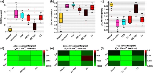
GLCM pixel statistics are summarized in Fig. 5. Subdiffuse reflectance of adipose tissue exhibits low contrast, low correlation, and high homogeneity relative to all malignant diagnoses, shown in Figs. 5(a)–5(c), respectively. These results are expected given that adipose tissue is predominately forward scattering with relatively low intensity, unstructured reflectance. Figure 5(d) indicates that adipose tissue can be separated from all three malignant diagnoses with statistical significance using GLCM metrics. Subdiffuse reflectance from connective tissue and FCD exhibits high contrast, high correlation, and low homogeneity relative to all malignant diagnoses. The combination of weakly backscattering collagen fibers and strongly backscattering collagen fibrils in connective tissue and the fibrotic nature of FCD might explain these statistics. Notably, the three GLCM statistics separate FCD from the malignant diagnoses, including ILC. The probability of a breast cancer patient having both FCD and ILC is relatively uncommon.¹⁵ However, the capability of GLCM metrics to statistically separate these two diagnoses is important; part I of this paper reported that optical scatter and color properties alone were unable to statistically separate these two diagnoses.

Fig. 5.

Boxplots for GLCM: (a) contrast, (b) correlation, and (c) homogeneity statistics for $f_x=1.37{\mathrm{mm}}^{-1}$, $\lambda =490\mathrm{nm}$ samples tallied in Table 1. Statistical discrimination between the three benign and three malignant tissue subtypes using (Con)trast, (Cor)relation, and (Hom)ogeneity was determined using a Mann–Whitney U-test. $p$-value heat maps are shown for (d) adipose, (e) connective, and (f) FCD, versus intermediate-grade IDC, high-grade IDC, and ILC.

3.2.2. Image primitives

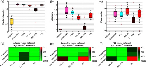
Image primitive metrics are summarized in Fig. 6. The Bernsen local thresholding rendered many of the low intensity, low contrast adipose tissue samples featureless. This explains the low fractal dimension, unit lacunarity, and zero Euler number for this tissue subtype in Figs. 6(a)–6(c), respectively. High-grade IDC samples follow a similar trend but to a lesser extent. The highly structured reflectances characteristic of connective tissue and FCD result in relatively high lacunarity, shown in Fig. 6(b). These results are expected given the rotational variance of these samples. Intermediate-grade IDC and ILC exhibit pockmarked textures (Fig. 2) that result in elevated Euler numbers, indicated in Fig. 6(c). Figure 6(f) shows that fractal dimension and lacunarity also statistically separate the rare combination of FCD and ILC.

Fig. 6.

Boxplots for structural image primitive metrics of (a) fractal dimension, (b) lacunarity, and (c) Euler number for $f_x=1.37{\mathrm{mm}}^{-1}$, $\lambda =490\mathrm{nm}$ samples tallied in Table 1. Statistical discrimination between these metrics are shown in Mann–Whitney U-test $p$-value heat maps for (d) adipose, (e) connective, and (f) FCD versus intermediate-grade IDC, high-grade IDC, and ILC.

3.2.3. Power spectral density curve parameters

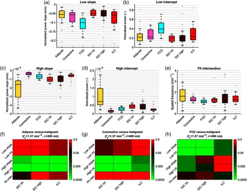
Figure 7 contains the PSD curve parameters derived from the subdiffuse reflectance samples. In Fig. 7(a), FCD samples present with relatively steep LSF slope, indicative of less LSF range content overall. In Fig. 7(h), LSF slope and intercept are both statistically distinct between FCD and the three malignant tissues. HSF slope and intercept separate both adipose tissue and connective tissue samples from the malignant tissue samples. Adipose tissue presents with a steeper HSF slope, because adipose tissue reflectance contains relatively less HSF range content. Connective tissue samples exhibit a more gradual HSF slope relative to the malignant tissues, because connective tissue reflectance contains additional HSF features relative to the malignant tissues.

Fig. 7.

Boxplots of normalized PSD curve linear fit parameters for $f_x=1.37{\mathrm{mm}}^{-1}$, $\lambda =490\mathrm{nm}$ samples tallied in Table 1. Parameters include LSF range (a) slope and (b) intercept, HSF (c) slope and (d) intercept, and (e) the spatial frequency at which the two fits intersect. Statistical discrimination between these metrics is shown in Mann–Whitney U-test $p$-value heat maps for (f) adipose, (g) connective, and (h) FCD, versus intermediate-grade IDC, high-grade IDC, and ILC.

3.3. Classification Analysis

The ROC curves in Fig. 8 reflect optimal classification performance based on a feature selection grid search. Table 3 summarizes optimal classification performance in the form of AUC, sensitivity, specificity, and accuracy with 95% confidence intervals. Adipose tissue versus intermediate-grade IDC and ILC can be classified with relatively high accuracy compared to adipose tissue versus high-grade IDC. Connective tissue can be classified against high-grade IDC with relatively high accuracy compared to connective tissue versus ILC. FCD can be classified relatively well against high-grade IDC, whereas the model is less effective at classifying FCD versus ILC. Accuracy confidence intervals are wide for some tissue subtypes given the sample sizes.

Fig. 8.

Classification performance using subdiffuse reflectance ($f_x=1.37{\mathrm{mm}}^{-1}$, $\lambda =490\mathrm{nm}$) and evaluated by ROC curve analysis for (a) adipose, (b) connective, and (c) FCD, versus the three malignant tissue subtypes. Classification used a linear SVM classifier, correlation-based feature selection with grid-searching, fivefold CV, sample size matching, and averaging over $n=100$ iterations. At most 11 texture features were included in each classification.

Table 3.

Summary of classification performance using subdiffuse SFDI-derived reflectance, a linear SVM classifier, correlation-based feature selection with grid searching for the optimal feature set, and a total of 11 possible texture features. Accuracy 95% confidence intervals are given in parentheses.

	Adipose versus			Connective versus			FCD versus
	IDC int	IDC high	ILC	IDC int	IDC high	ILC	IDC int	IDC high	ILC
AUC	0.97	0.77	0.98	0.79	0.93	0.58	0.91	0.93	0.67
Sensitivity	0.99	0.74	0.99	0.72	0.89	0.59	0.89	0.92	0.61
Specificity	0.86	0.67	0.90	0.71	0.95	0.50	0.79	0.92	0.65
Accuracy	0.92	0.70	0.95	0.72	0.92	0.55	0.84	0.92	0.63
	(0.88 to 0.96)	(0.58 to 0.82)	(0.90 to 1.00)	(0.54 to 0.90)	(0.89 to 0.95)	(0.41 to 0.69)	(0.75 to 0.93)	(0.90 to 0.94)	(0.47 to 0.79)

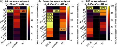
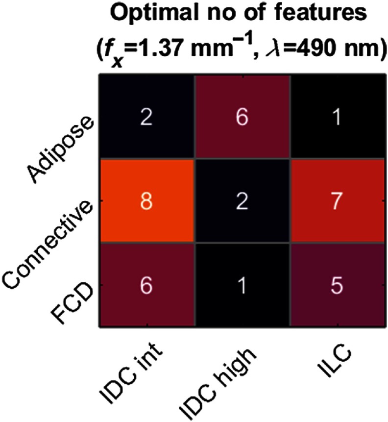
The texture features used in optimal classifications are reported in Fig. 9 in heat map form. The most frequently used metrics in benign–malignant classification pairs are boxed in gray, and the percent of the $n=100$ classifications that employed the given metric is displayed. Figure 9(a) indicates that the most valuable metric for classifying adipose tissue versus intermediate-grade IDC or ILC is GLCM correlation, and classifying adipose versus high-grade IDC involved a more distributed selection of metrics. In Fig. 9(b), a range of metrics were used to classify connective tissue versus intermediate-grade IDC and ILC. GLCM correlation was always found in the optimal classification of connective tissue versus high-grade IDC. In Fig. 9(c), GLCM contrast and correlation were the most important features for classifying FCD against the malignant tissue subtypes. Figure 10 reports the optimal number of features used in every benign–malignant classification. Values are averaged over all $n=100$ iterations and rounded to the nearest integer. No classification scenario used more than eight texture features on average. The benign–malignant pair that used the most features for optimal classification was connective tissue versus ILC, which demonstrated the poorest classification performance overall.

Fig. 9.

Feature selection for classification of samples using only subdiffuse reflectance texture metrics ($f_x=1.37{\mathrm{mm}}^{-1}$, $\lambda =490\mathrm{nm}$). The percent of $n=100$ classification iterations that used specific texture metrics are shown in heat map form for (a) adipose, (b) connective, and (c) FCD versus the three malignant tissue subtypes. Texture features listed to the left of (a) apply to all subplots. Boxed percentages identify how frequently the most important metric(s) were used in each benign–malignant classification scenario.

Fig. 10.

Optimal number of features (averaged over $n=100$ classification iterations and rounded to the nearest integer) determined by correlation-based feature selection and grid searching for sample classification using subdiffuse ($f_x=1.37{\mathrm{mm}}^{-1}$, $\lambda =490\mathrm{nm}$) reflectance texture metrics.

3.4. Limitations and Future Work

The classification model used a linear SVM for binary classification, but tissue diagnostics is inherently a multiclass classification problem. The current model could be clinically relevant given the tissue subtype-limiting benefits of preoperative biopsy. Nevertheless, potential clinical value would be increased if it were a multiclass classification model. Classification involved fivefold CV due to sample size limitations. With increased tissue sample sizes, leave-one-out-CV (LOOCV), which partitions the data by patient, specimen, or RoI, should be implemented. Often, partitioning is done on the patient level and is referred to as leave-one-patient-out CV. LOOCV avoids confounding scenarios when unique features contained within a single patient or RoI are spread across multiple folds, thus appearing in both the training and testing datasets and potentially leading to interpatient model bias.⁴³

Classification results reveal that reflectance texture analysis has both strengths and weaknesses. Subdiffuse reflectance is directly related to microscopic structures in tissue but does not necessarily provide unique signals associated with all tissue subtypes diagnosed on the histopathological level. Adipose tissue and high-grade IDC cannot be accurately resolved using subdiffuse reflectance alone using the model presented here. The same applies for differentiating between connective tissue or FCD from ILC. Combining tissue texture features with other tissue properties may overcome these limitations. For instance, quantitative color properties can readily separate adipose tissue and high-grade IDC.¹⁵ Future studies could focus on the collection of a larger hold-out dataset, such that the classification model is trained and tested on a subset of the data and a second subset is reserved purely for assessing classification performance.

The potential benefits of subdiffuse reflectance texture quantification over optical property quantification include a simplified data collection protocol, computational efficiency, and avoiding light transport model assumptions, which may lead to additional errors. Still, it is known that optical properties offer invaluable characterization of a wide range of biological tissues. Future work should compare surface tissue classification performance using sd-SFDI reflectance textures and optical properties. In summary, additional studies are required to validate these classification results on even larger sample sizes, to test the inclusion of other tissue properties in the classification model, and to improve the generalization and applicability of the techniques investigated in part II of this paper.

4. Conclusions

Today 15% to 35% of BCS patients require a second surgery due to incomplete initial excision of tumor tissue. Intraoperative optical imaging may help clinicians to reduce the positive margin rate in BCS by rapidly providing enhanced contrast to surface tissue features over a wide FOV. Sd-SFDI shows promise for this application. In part II of this paper, an sd-SFDI imaging and analysis protocol for BCS tissue surface characterization was introduced that uses one subdiffuse spatial frequency, one blue optical wavelength, and reflectance texture. The protocol leverages wide FOV sd-SFDI scatter as a contrast mechanism and benefits from relatively fast acquisition and processing times compared to optical property quantification. The protocol avoids light transport model assumptions for metric quantitation, because it analyzes intrinsic reflectance textures in the imaged tissue. Finally, different combinations of pixel statistics, image primitives, and PSD curve parameters provided statistical significance between three benign and three malignant breast tissue subtypes, and classification results provide one method of determining the relative importance of these metrics for characterizing resected BCS tissues. Reflectance texture in combination with other tissue features, such as color properties, may offer clinically valuable diagnostics for intraoperative BCS margin guidance.

Biography

Biographies of the authors are not available.

Disclosures

The authors declare no conflicts of interests.

References

- 1.American Cancer Society, “Breast cancer facts and figures 2017–2018,” American Cancer Society, Inc., Atlanta: (2017). [Google Scholar]
- 2.Fisher B., et al. , “Twenty-year follow-up of a randomized trial comparing total mastectomy, lumpectomy, and lumpectomy plus irradiation for the treatment of invasive breast cancer,” N. Engl. J. Med. 347(16), 1233–1241 (2002). 10.1056/NEJMoa022152 [DOI] [PubMed] [Google Scholar]
- 3.Balch G. C., Mithani S. K., Kelley M. C., “Accuracy of intraoperative gross examination of surgical margin status in women undergoing partial mastectomy for breast malignancy,” Am. J. Surg. 71(1), 22–28 (2005). [PubMed] [Google Scholar]
- 4.Fleming F. J., et al. , “Intraoperative margin assessment and re-excision rate in breast conserving surgery,” Eur. J. Surg. Oncol. 30(3), 233–237 (2004). 10.1016/j.ejso.2003.11.008 [DOI] [PubMed] [Google Scholar]
- 5.Lovrics P. J., et al. , “The relationship between surgical factors and margin status after breast-conservation surgery for early stage breast cancer,” Am. J. Surg. 197(6), 740–746 (2009). 10.1016/j.amjsurg.2008.03.007 [DOI] [PubMed] [Google Scholar]
- 6.Lovrics P. J., et al. , “Technical factors, surgeon case volume and positive margin rates after breast conservation surgery for early-stage breast cancer,” Can. J. Surg. 53(5), 305–312 (2010). [PMC free article] [PubMed] [Google Scholar]
- 7.Maloney B. W., et al. , “Review of methods for intraoperative margin detection for breast-conserving surgery,” J. Biomed. Opt. 23(10), 100901 (2018). 10.1117/1.JBO.23.10.100901 [DOI] [PMC free article] [PubMed] [Google Scholar]
- 8.Kaczmarski K., et al. , “Surgeon re-excision rates after breast-conserving surgery: a measure of low-value care,” J. Am. Coll. Surg. 228(4), 504–512.e2 (2019). 10.1016/j.jamcollsurg.2018.12.043 [DOI] [PubMed] [Google Scholar]
- 9.Schnabel F., et al. , “A randomized prospective study of lumpectomy margin assessment with use of marginprobe in patients with nonpalpable breast malignancies,” Ann. Surg. Oncol. 21, 1589–1595 (2014). 10.1245/s10434-014-3602-0 [DOI] [PMC free article] [PubMed] [Google Scholar]
- 10.Kaufman Z., et al. , “Mapping breast tissue types by miniature radio-frequency near-field spectroscopy sensor in ex vivo freshly excised specimens,” BMC Med. Imaging 16, 57 (2016). 10.1186/s12880-016-0160-x [DOI] [PMC free article] [PubMed] [Google Scholar]
- 11.Kennedy S., et al. , “Optical breast cancer margin assessment: an observational study of the effects of tissue heterogeneity on optical contrast,” Breast Cancer Res. 12, R91 (2010). 10.1186/bcr2770 [DOI] [PMC free article] [PubMed] [Google Scholar]
- 12.Wang Y., et al. , “Quantitative molecular phenotyping with topically applied SERS nanoparticles for intraoperative guidance of breast cancer lumpectomy,” Sci. Rep. 6, 21242 (2016). 10.1038/srep21242 [DOI] [PMC free article] [PubMed] [Google Scholar]
- 13.John E. R. S., et al. , “Diagnostic accuracy of intraoperative techniques for margin assessment in breast cancer surgery,” Ann. Surg. 265(2), 300–310 (2017). 10.1097/SLA.0000000000001897 [DOI] [PubMed] [Google Scholar]
- 14.Jorns J. M., Visscher D. W., Sabel M., “Intraoperative frozen section analysis of margins in breast-conserving surgery significantly decreases reoperative rates: one-year experience at an ambulatory surgical center,” Am. J. Clin. Pathol. 138, 657–669 (2012). 10.1309/AJCP4IEMXCJ1GDTS [DOI] [PMC free article] [PubMed] [Google Scholar]
- 15.Maloney B. W., et al. , “Structured light imaging for breast-conserving surgery part I: optical scatter and color analysis,” J. Biomed. Opt. 24(9), 096002 (2019). 10.1117/1.JBO.24.9.096002 [DOI] [PMC free article] [PubMed] [Google Scholar]
- 16.Cuccia D. J., et al. , “Quantitation and mapping of tissue optical properties using modulated imaging,” J. Biomed. Opt. 14(2), 024012 (2009). 10.1117/1.3088140 [DOI] [PMC free article] [PubMed] [Google Scholar]
- 17.Kanick S. C., et al. , “Sub-diffusive scattering parameter maps recovered using wide-field high-frequency structured light imaging,” Biomed. Opt. Express 5(10), 3376–3390 (2014). 10.1364/BOE.5.003376 [DOI] [PMC free article] [PubMed] [Google Scholar]
- 18.Krishnaswamy V., et al. , “Structured light scatteroscopy,” J. Biomed. Opt. 19(7), 070504 (2014). 10.1117/1.JBO.19.7.070504 [DOI] [PubMed] [Google Scholar]
- 19.Jacques S. L., “Optical properties of biological tissues: a review,” Phys. Med. Biol. 58, R37–R61 (2013). 10.1088/0031-9155/58/11/R37 [DOI] [PubMed] [Google Scholar]
- 20.Bodenschatz N., et al. , “Quantifying phase function influence in subdiffusively backscattered light,” J. Biomed. Opt. 21(3), 035002 (2016). 10.1117/1.JBO.21.3.035002 [DOI] [PubMed] [Google Scholar]
- 21.McClatchy D. M., et al. , “Calibration and analysis of a multimodela mico-CT and structured light imaging system for the evaluation of excised breast tissue,” Phys. Med. Biol. 62, 8983–9000 (2017). 10.1088/1361-6560/aa94b6 [DOI] [PMC free article] [PubMed] [Google Scholar]
- 22.McClatchy D. M., et al. , “Wide-field quantitative imaging of tissue mircostructure using sub-diffuse spatial frequency domain imaging,” Optica 3(6), 613–621 (2016). 10.1364/OPTICA.3.000613 [DOI] [PMC free article] [PubMed] [Google Scholar]
- 23.Laughney A. M., et al. , “Spectral discrimination of breast patahologies in situ using spatial frequency domain imaging,” Breast Cancer Res. 15(4), R61 (2013). 10.1186/bcr3455 [DOI] [PMC free article] [PubMed] [Google Scholar]
- 24.McClatchy D. M., et al. , “Light scattering measured with spatial frequency domain imaging can predict stromal versus epithelial proportions in surgically resected breast tissue,” J. Biomed. Opt. 24(7), 071605 (2018). 10.1117/1.JBO.24.7.071605 [DOI] [PMC free article] [PubMed] [Google Scholar]
- 25.Angelo J. P., et al. , “Review of structured light in diffuse optical imaging,” J. Biomed. Opt. 24(7), 071602 (2018). 10.1117/1.JBO.24.7.071602 [DOI] [PMC free article] [PubMed] [Google Scholar]
- 26.Cuccia D. J., et al. , “Modulated imaging: quantitative analysis and tomography of turbid media in the spatial-frequency domain,” Opt. Lett. 30(11), 1354–1356 (2005). 10.1364/OL.30.001354 [DOI] [PubMed] [Google Scholar]
- 27.Laughney A. M., et al. , “Scatter spectroscopic imaging distinguishes between breast pathologies in tissues relevant to surgical margin assessment,” Clin. Cancer Res. 18(22), 6315–6325 (2012). 10.1158/1078-0432.CCR-12-0136 [DOI] [PMC free article] [PubMed] [Google Scholar]
- 28.Castellano G., et al. , “Texture analysis of medical images,” Clin. Radiol. 59(12), 1061–1069 (2004). 10.1016/j.crad.2004.07.008 [DOI] [PubMed] [Google Scholar]
- 29.Baish J. W., Jain R. K., “Fractals and cancer,” Cancer Res. 60, 3683–3688 (2000). [PubMed] [Google Scholar]
- 30.Torres-Mejia G., et al. , “Mammographic features and subsequent risk of breast cancer: a comparison of qualitative and quantitative evaluations in the Guernsey prospective studies,” Cancer Epidemiol. Biomarkers Prev. 14(5), 1052–1059 (2005). 10.1158/1055-9965.EPI-04-0717 [DOI] [PubMed] [Google Scholar]
- 31.Chan A., Tuszynski J. A., “Automatic prediction of tumour malignancy in breast cancer with fractal dimension,” R. Soc. Open Sci. 3, 160558 (2016). 10.1098/rsos.160558 [DOI] [PMC free article] [PubMed] [Google Scholar]
- 32.Elson J. M., Bennett J. M., “Calculation of the power spectral density from surface profile data,” Appl. Opt. 34(1), 201–208 (1995). 10.1364/AO.34.000201 [DOI] [PubMed] [Google Scholar]
- 33.Haralick R. M., Shanmugam K., Dinstein I., “Textural features for image classification,” IEEE Trans. Syst. Man Cybern. SMC-3(6), 610–621 (1973). 10.1109/TSMC.1973.4309314 [DOI] [Google Scholar]
- 34.MATLAB, “Image processing toolbox v10.2,” MathWorks, 2018, https://www.mathworks.com/products/image.html (accessed 1 December 2018). [Google Scholar]
- 35.Sezgin M., Sankur B., “Survey over image thresholding techniques and quantitative performance evaluation,” J. Electron. Imaging 13(1), 146–165 (2004). 10.1117/1.1631315 [DOI] [Google Scholar]
- 36.Bernsen J., “Dynamic thresholding of gray level images,” in Proc. Int. Conf. Pattern Recognit., pp. 1251–1255 (1986). [Google Scholar]
- 37.Costa A., Hausdorff (Box-Counting) Fractal Dimension, MATLAB File Exchange, https://www.mathworks.com/matlabcentral/fileexchange/30329-hausdorff-box-counting-fractal-dimension (accessed 1 December 2018).
- 38.Costa A. F., Mamani G. H., Traina A., “An efficient algorithm for fractal analysis of textures,” in 25th SIBGRAPI Conf. Graphics, Patterns and Images, Ouro Preto: (2012). [Google Scholar]
- 39.Vadakkan T., Lacunarity of a Binary Image, MATLAB File Exchange, https://www.mathworks.com/matlabcentral/fileexchange/25261-lacunarity-of-a-binary-image (accessed 1 December 2018).
- 40.Ruzanski E., Radially Averaged Power Spectrum of 2D Real-Valued Matrix, MATLAB File Exchange, https://www.mathworks.com/matlabcentral/fileexchange/23636-radially-averaged-power-spectrum-of-2d-real-valued-matrix (accessed 1 December 2018).
- 41.Rowland R., et al. , “Burn wound classification model using spatial frequency-domain imaging and machine learning,” J. Biomed. Opt. 24(5), 056007 (2019). 10.1117/1.JBO.24.5.056007 [DOI] [PMC free article] [PubMed] [Google Scholar]
- 42.MATLAB, “Statistics and machine learning toolbox v11.3,” MathWorks, 2018, https://www.mathworks.com/help/stats/index.html (accessed 1 December 2018). [Google Scholar]
- 43.Hastie T., Tibshirani R., Friedman J., “Cross-validation,” in The Elements of Statistical Learning, 2nd ed., p. 243, Springer, New York: (2009). [Google Scholar]
- 44.Hall M. A., Smith L. A., “Feature selection for machine learning: comparing a correlation-based filter approach to the wrapper,” in Proc. Twelfth Int. Florida Artif. Intell. Res. Soc. Conf., pp. 235–239 (1999). [Google Scholar]
- 45.Fawcett T., “An introduction to ROC analysis,” Pattern Recognit. Lett. 27, 861–874 (2006). 10.1016/j.patrec.2005.10.010 [DOI] [Google Scholar]
- 46.Schmitt J. M., Kumar G., “Optical scattering properties of soft tissue: a discrete particle model,” Appl. Opt. 37(13), 2788–2798 (1998). 10.1364/AO.37.002788 [DOI] [PubMed] [Google Scholar]
- 47.Boecker W. J., Dabbs D. J., “Fibrocystic change and usual epithelial hyperplasia of Ductal type,” Chapter 18 in Breast Pathology, Dabbs D. J., Ed., 2nd ed., pp. 373–395, Elsevier, Inc., Philadelphia: (2017). [Google Scholar]