Identification of caveolin-1 domain signatures via machine learning and graphlet analysis of single-molecule super-resolution data

Abstract

Motivation

Network analysis and unsupervised machine learning processing of single-molecule localization microscopy of caveolin-1 (Cav1) antibody labeling of prostate cancer cells identified biosignatures and structures for caveolae and three distinct non-caveolar scaffolds (S1A, S1B and S2). To obtain further insight into low-level molecular interactions within these different structural domains, we now introduce graphlet decomposition over a range of proximity thresholds and show that frequency of different subgraph (k = 4 nodes) patterns for machine learning approaches (classification, identification, automatic labeling, etc.) effectively distinguishes caveolae and scaffold blobs.

Results

Caveolae formation requires both Cav1 and the adaptor protein CAVIN1 (also called PTRF). As a supervised learning approach, we applied a wide-field CAVIN1/PTRF mask to CAVIN1/PTRF-transfected PC3 prostate cancer cells and used the random forest classifier to classify blobs based on graphlet frequency distribution (GFD). GFD of CAVIN1/PTRF-positive (PTRF+) and -negative Cav1 clusters showed poor classification accuracy that was significantly improved by stratifying the PTRF+ clusters by either number of localizations or volume. Low classification accuracy (<50%) of large PTRF+ clusters and caveolae blobs identified by unsupervised learning suggests that their GFD is specific to caveolae. High classification accuracy for small PTRF+ clusters and caveolae blobs argues that CAVIN1/PTRF associates not only with caveolae but also non-caveolar scaffolds. At low proximity thresholds (50–100 nm), the caveolae groups showed reduced frequency of highly connected graphlets and increased frequency of completely disconnected graphlets. GFD analysis of single-molecule localization microscopy Cav1 clusters defines changes in structural organization in caveolae and scaffolds independent of association with CAVIN1/PTRF.

Supplementary information

Supplementary data are available at Bioinformatics online.

1 Introduction

Graphs (or networks) are ubiquitous and powerful mathematical structures used for modeling objects and their interactions. In graph representation, objects are modeled via nodes, and interactions between objects are modeled via connections or edges between the nodes. Graph analysis methods have been successfully applied to the analysis of social, computer, brain and biological networks (Bassett and Sporns, 2017; Brown et al., 2014; Costa et al., 2008; Krivitsky et al., 2009; Newman, 2003; Zitnik and Leskovec, 2017). Point clouds refer to datasets where a collection of objects or nodes are presented without connections. Many methods have been deployed to extract features from point clouds, either via hand-crafted features or automatically derived features via deep learning, for different machine learning tasks such as segmentation and classification (Gumhold et al., 2001; Qi et al., 2017).

Graphlets and motifs are two related concepts used to describe small patterns or subnetworks that occur in large networks. Graphlets, small connected non-isomorphic induced subgraphs of a large network, were introduced by Pržulj et al. (2004) as measures of local network structure. Network motifs, on the other hand, are interconnected patterns significantly and highly recurrent in real-world networks compared with random networks (Milo et al., 2002). Consequently, graphlets and motifs are regarded as the basic building blocks for large networks and graphs. Decomposing large networks into their base graphlets and calculating occurrence frequencies [i.e. graphlet frequency distribution (GFD)], provide robust features to differentiate between networks and discover their underlying signatures.

Graphlet patterns can vary based on the number of the nodes k and their connectivity in each subgraph. The number of possible connectivity patterns of a graphlet increases exponentially with k and hence increases the complexity of enumerating the graphlets in big graphs. Typically, graphlet patterns are extracted for $k=2,3,4,$ and 5 nodes. Moreover, finding some of the patterns are NP-hard problems (e.g. finding the clique, or fully interconnected set of vertices, of maximum size) and require efficient approximate counting algorithms (Ahmed et al., 2015, 2017). Many methods have been proposed to find graphlet patterns in networks (Ahmed et al., 2015; Hočevar and Demšar, 2014; Marcus and Shavitt, 2012; Shervashidze et al., 2009). In particular, the parallel graphlet decomposition method (Ahmed et al., 2015, 2017) is very fast, scalable and supports extracting macro and micro graphlets features and counting both connected and disconnected graphlets.

Graphlets have been widely used for a myriad of applications such as network similarity, network alignment, biological and protein networks, prediction and classification, image segmentation, etc. (Bressan et al., 2017; Dutta and Sahbi, 2017; Kollias et al., 2012; Pržulj, 2007; Pržulj et al., 2004; Shervashidze et al., 2009; Shin et al., 2016; Zhang et al., 2013). Recently, graphlets/motifs are exploited as a high-order connectivity patterns information for network clustering (Benson et al., 2016), and fast local graph clustering and community detection tasks (Yin et al., 2017).

Recently, we described a graph-based complex network analysis clustering method (Khater et al., 2018) to analyze the 3D point cloud of single-molecule localization microscopy (SMLM) super-resolution microscopy data. The method consists of an integrated pipeline that includes network construction, multiple blink correction, noise filtering and cluster segmentation, analysis and identification using machine learning. Application of unsupervised learning network analysis and machine learning to point clouds of caveolin-1 (Cav1), the coat protein of cell surface caveolae invaginations, reported a modular structure for caveolae, similar to that determined by cryoEM (Ludwig et al., 2016; Stoeber et al., 2016), as well as three non-caveolar scaffolds, including a previously unreported hemispherical scaffold domain (Khater et al., 2018). Caveolae invagination requires the adaptor protein CAVIN1 [also known as Polymerase I and Transcript Release Factor protein (PTRF) and referred to in this manuscript as CAVIN1/PTRF and, for brevity, PTRF]. Here we apply supervised machine learning approaches, leveraging GFD features and a CAVIN1/PTRF total internal reflection fluorescence mask to form training data, to identify CAVIN1/PTRF-associated Cav1 domains and use graphlet analysis to classify and compare the Cav1-labeled domains. We show that graphlets are highly efficient classifiers that distinguish caveolae from scaffolds. Comparison of unsupervised and supervised learning, the latter using a CAVIN1/PTRF mask, suggests that CAVIN1/PTRF associates not only with caveolae but also with scaffold domains.

2 Materials and methods

We summarize the abbreviations and acronyms used in this paper in Table 1.

Table 1.

The list of abbreviations and acronyms used in this paper

Term	Explanation
PC3	Prostate cancer cell lines
PC3-PTRF	CAVIN1/PTRF-transfected PC3 cells
Cav1	Caveolin-1 protein
PTRF	Polymerase I and Transcript Release Factor protein
	Also known as CAVIN1
PTRF+	PTRF-positive (blobs inside the CAVIN1/PTRF mask)
PTRF−	PTRF-negative (blobs outside the CAVIN1/PTRF mask)
PT	Proximity threshold
GSD	Ground State depletion
TIRF	Total internal reflection fluorescence
SMLM	Single-molecule localization microscopy
GFD	Graphlet frequency distribution
Acc	Accuracy (classification evaluation measure)
Spe	Specificity (classification evaluation measure)
Sen	Sensitivity (classification evaluation measure)
AUC	Area under ROC curve (classification evaluation measure)
ROC	Receiver operating characteristic (classification evaluation measure)
t-SNE	t-distributed Stochastic Neighbor Embedding, a dimensionality reduction and visualization technique (Maaten and Hinton, 2008)

Figure 1A and B shows an overview of the framework for GFD classification of SMLM Cav1-labeled blobs. SMLM event lists of anti-Cav1 labeling of CAVIN1/PTRF-transfected PC3 prostate cancer cells (PC3-PTRF cells) (are converted into 3D point cloud representation of blink locations in 3D space. Following network construction from the Cav1 point clouds, multiple blinking from single fluorophores and closely associated fluorophores is corrected, noise/background is filtered out and clusters identified, as previously described (Khater et al., 2018). We then applied our established unsupervised learning approach based on topological, shape and network features to identify Cav1 clusters (blobs). We previously learned four groups of Cav1 blobs and, through matching the learned groups from both PC3 and PC3-PTRF populations, we identified the blobs types, (table in Fig. 1E), as PP1 (S2 Scaffolds), PP2 (caveolae), PP3 (S1B scaffolds) or PP4 (S1A scaffolds) (Khater et al., 2018). Alternatively, we used a wide-field CAVIN1/PTRF mask for supervised learning in which blobs were classed as either ‘in mask’ or ‘out mask’. Every blob is processed as shown in Figure 1C, where a network is constructed for every blob and the different graphlet patterns are extracted for k = 4 nodes (Fig. 2B). The graphlet patterns are then counted and used to find the GFD for the connected and disconnected graphlet patterns of every blob. Figure 1D shows representative images of all Cav1 clusters, Cav1 clusters in PTRF-positive (PTRF+) and out PTRF-negative (PTRF−) of the CAVIN1/PTRF mask and unsupervised learning classification of blobs as PP1, PP2, PP3 or PP4 (Fig. 2A). Quantification of blob distribution showed that all four classes of Cav1 blobs were present in and out of the CAVIN1/PTRF mask, with caveolae (PP2) more present in the PTRF+ blobs, small S1A (PP4) and S1B (PP3) scaffolds less present and hemispherical S2 scaffolds (PP1) present amongst both PTRF+ and PTRF− blobs (Fig. 1E). In light of the heterogeneous distribution of the various classes of Cav1 blobs in and out of the CAVIN1/PTRF mask, we decided to classify the blobs using random forest classification based on GFD features.

Fig. 1.

SMLM Cav1 blob identification via graphlet analysis. (A) An overview of the proposed method. The Cav1 protein is labeled for SMLM imaging. The CAVIN1/PTRF mask is used to obtain the ground truth labels for blobs to define PTRF+ and PTRF− classes. The SMLM data are processed using Khater et al. (2018) to obtain the segmented Cav1 blobs and their classes to train the supervised machine learning model. The GFD features for the Cav1 blobs are used to train a machine learning classifier for blob identification. (B) The proposed analysis framework. Cav1 protein is labeled in PC3 prostate cancer cells and PC3-PTRF cells. SMLM events are represented as a 3D point cloud of Cav1 blinks and 3D SMLM Network Analysis computational pipeline (Khater et al., 2018) used for cluster analysis of labeled Cav1 proteins, including modules to correct for multiple blinking of single fluorophores, filtering, segmenting and identifying the blobs using unsupervised learning (Khater et al., 2018). We also used the wide-field CAVIN1/PTRF total internal reflection fluorescence mask to classify Cav1 blobs for the supervised learning task. Graphlet features were extracted for every blob network at various PTs. We used a parallel graphlet decomposition library (Ahmed et al., 2015) to extract feature vector for every network. Feature vectors from all the blobs were used for machine learning classification and identifying biosignatures for the different Cav1 structures. (C) To get graphlet features for a single blob, a network is constructed for the 3D point cloud of a single blob and graphlets are then counted in every network. GFD features are derived from connected ($g{4}_1,g{4}_2,g{4}_3,g{4}_4,g{4}_5,g{4}_6$) and disconnected ($g{4}_7,g{4}_8,g{4}_9,g{4}_{10},g{4}_{11}$) graphlet patterns for k = 4 nodes. GFD features can be extracted for connected graphlets alone, disconnected graphlets alone and for both connected and disconnected graphlets. We showed the process of extracting graphlet features for some of the Cav1 blobs in Figure 2B. (D) 3D views of a PC3-PTRF cell showing all Cav1 blobs, PTRF+ Cav1 blobs in-mask (blue) with remaining blobs, out-mask, labeled as PTRF− (green) and blobs classified based on unsupervised learning as PP1, PP2, PP3 and PP4 blobs (Khater et al., 2018). (E) Percentages of blobs for each group in- and out-mask and distribution of blobs within and without the CAVIN1/PTRF mask are shown

Fig. 2.

The process of extracting the graphlet features from the various blob types. (A) The segmented and labeled blobs from PC3 and PC3-PTRF cells in the dataset are used for feature extraction. We show a representative blob from each group. The blobs are labeled based on the CAVIN1/PTRF mask into PTRF+ and PTRF− classes or labeled based on the unsupervised labeling method (Khater et al., 2018) into four classes (i.e. PP1, PP2, PP3 and PP4). (B) Networks at PTs of 40 and 80 nm are shown and examples of graphlets in the networks are given. Graphlet features for k = 2, 3, 4 nodes were extracted and counted from the blobs. The GFD features were extracted for k = 4 nodes

To extract the graphlet features, we constructed networks for every blob based on the proximity threshold (PT) between each pair of molecules within the blob. The nodes represent molecules in the network, where interaction between the neighboring molecules is represented as an edge (Figs 1C and 2B). We leveraged the parallel graphlet decomposition method (Ahmed et al., 2015, 2017) to extract graphlet features from the blobs’ networks. The parallel graphlet decomposition method extracts macro (global) motif counts for the motifs with $k=2,k=3$ and k = 4 nodes, micro-motif counts and the GFD features. As the micro and macro features are highly dependent on the number of nodes in the network, we based our analysis on GFD features with k = 4 nodes (Fig. 1C) so as not to bias our classification model between small and large blobs and analyzed GFD features regardless of the number of nodes in their corresponding networks. The extracted features are then used to classify the blobs. See Supplementary Methods for details.

3 Results

We first applied GFD analysis to the four classes of Cav1 domains previously identified in PC3-PTRF cells (PP1: S2 scaffolds; PP2: caveolae; PP3: S1A scaffolds; PP4: S1B scaffolds) based on topology, shape and network features (Khater et al., 2018). As can be seen in Figure 3A, frequency distributions for the 11 k = 4 graphlets vary amongst the four classes of blobs, shown here at PT = 80 nm. Given that we describe each blob with a vector of features and that this vector is high (multi) dimensional, visualizing these features is not straightforward as with 2 or 3D vectors. In our work, the vectors are 11D capturing the distribution of the frequency of the 11 graphlets used in this paper. A powerful and well-known approach for visualizing high-dimensional vectors is t-distributed Stochastic Neighbor Embedding (t-SNE) (Maaten and Hinton, 2008). t-SNE works by optimally projecting high-dimensional feature vectors to lower dimensional 2D so they can be easily displayed. The projection is optimal in that it minimizes the difference (measured via the Kullback–Leibler divergence) between the conditional probability distributions (probability of picking neighboring high-dimensional feature vector j given reference vector i) before and after the projection and hence retains the local structure and reveal the important global structure. In t-SNE plots, each point represents the feature vector of a blob (after projection to 2D space). t-SNE visualization for the GFD features clearly show distinct groups for caveolae (PP2), hemispherical S2 scaffolds (PP1) and overlap between the similar and smaller S1A (PP4) and S1B (PP3) scaffolds.

Fig. 3.

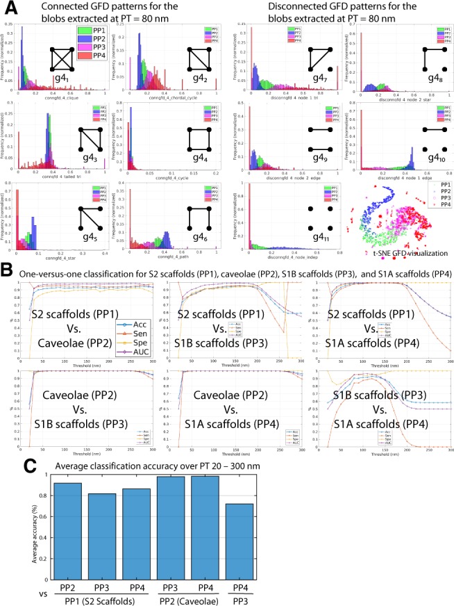
Graphlet biosignatures for the Cav1 domains via machine learning. (A) GFD features of S2 scaffolds (PP1), caveolae (PP2), S1B scaffolds (PP3) and S1A scaffolds (PP4) extracted using the 3D SMLM Network Analysis pipeline. Histograms of the connected and disconnected GFD features extracted from the networks at PT=80 nm are shown. t-SNE visualization of the GFD features shows a 2D view of the projected features that depicts how the blobs from different classes are distributed. (B) Machine learning classification of the four groups using the GFD features extracted at various PTs. In the classification task, we used the one-versus-one strategy for the four groups multi-labeled data to classify the blobs with four classes. In total, we have six classifiers that show all the pairs of groups of classification results. The binary classification shows the performance of classifying every group against the other groups at various PTs. We show the classification results for the binary classification task by reporting the Acc, Sen, Spe and AUC. We also showed the result of using one-versus-all and the multi-class classification results in the Supplementary Figure S1C. The bar plot shows the average classification Acc over the used PTs for the binary classifiers in (B) above. High classification Acc suggests that the groups are distinct and the classifier can discriminate and identify them. Low classification Acc suggests that the classifier misclassify some of the blobs and unable to discriminate them due to the similarity and overlapping of their GFD features

One-versus-one classification between the four groups (i.e. for M = 4 groups, we will have $N=\frac{M\times (M-1)}{2}=6$ classifiers) was determined across PTs from 20–300 nm, the minimal PT corresponds to the merge threshold applied and the maximum to the largest blob size. Caveolae (PP2) showed a high classification accuracy (Acc), sensitivity (Sen), specificity (Spe) and area under receiver operating characteristic curve (AUC) against all three scaffold groups (Fig. 3B). Classification Acc was highest versus S1 scaffolds (PP3, PP4) that were most poorly distinguished from each other (Fig. 3B and C). Progressive increases in classification Acc between caveolae (PP2) and S2 scaffolds and then S1 scaffolds is highlighted by the graph showing average classification Acc over the 20–300 nm PT range (Fig. 3C). Use of GFD feature based classification has therefore corroborated Cav1 cluster classification based on topology, size and shape features (Khater et al., 2018). We also used the one-versus-all classification (Supplementary Fig. S1B) and used the voting to combine the results of all the classifiers to get the multi-class classification Acc (Supplementary Fig. S1C). The results correspond to the one-versus-one classification results. Moreover, the multi-class classification results show that the classification loss (which measures the predictive inaccuracy of classification) is <10% when the PT is between 50 and 160 nm. GFD features best discriminate and identify Cav1 domains in the 50–160 nm PT range.

We then applied GFD classification to PTRF+ and PTRF− blobs. Figure 4A shows the processing of the CAVIN1/PTRF mask by applying the morphological closing operation to remove small holes in the mask and superposition of segmented Cav1 blobs on the CAVIN1/PTRF mask for correspondence analysis. Using this method, Cav1 blobs touching the mask are ‘in’ mask and others ‘out’ mask. Binary GFD pattern analysis shows a high degree of overlap between the PTRF+ and PTRF− classes for all graphlets. GFD similarity between the two classes is highlighted by extensive overlap in the t-SNE visualization and the low (65%) classification Acc between the two groups (Fig. 4B and C).

Fig. 4.

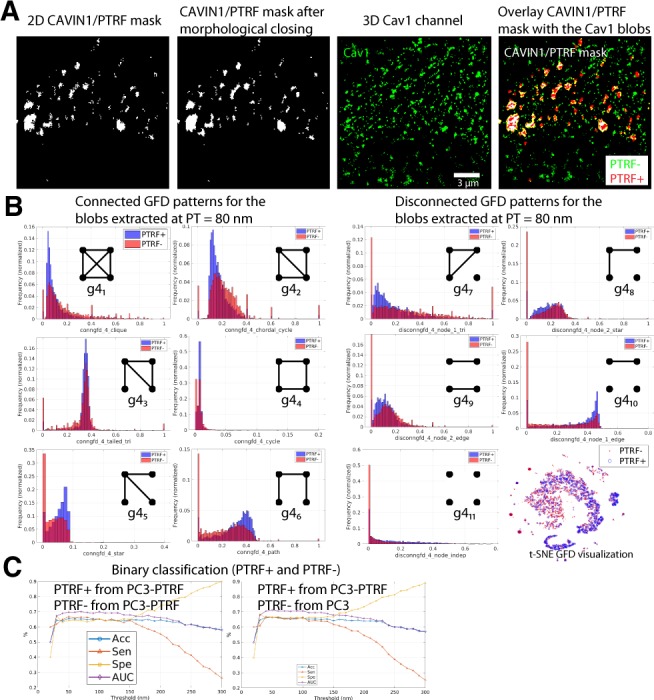
Classification results using GFD features at various PTs for PTRF+ and PTRF− blobs. (A) A wide-field CAVIN1/PTRF mask (white) is used to label blobs as PTRF+ or CAVIN1/PTRF− (supervised labeling) or to assign the learned and matched groups as S2 scaffolds (PP1), caveolae (PP2), S1B scaffolds (PP3) and S1A scaffolds (PP4) blobs (unsupervised labeling) as in Figure 1D. (B) GFD features for the blobs when using the CAVIN1/PTRF mask to label the blobs into PTRF+ and PTRF− are shown as histograms of connected and disconnected GFD features extracted from the networks at PT=80 nm. t-SNE visualization of the GFD features shows that the blobs are not well separated when using the CAVIN1/PTRF mask to label the blobs. (C) We used the CAVIN1/PTRF mask to label the blobs as PTRF+ and PTRF− then applied machine learning classification after extracting GFD features. We show the classification results for the binary classification task by reporting the Acc, Sen, Spe and AUC

CAVIN1/PTRF is required for caveolae formation and known to associated with caveolae (Hansen et al., 2013; Hill et al., 2008; Liu and Pilch, 2008). Caveolae are larger than scaffolds (Khater et al., 2018) and volume and number of nodes (molecular localizations) analysis of the four classes of blobs defined by unsupervised learning identified a clear size demarcation between caveolae (PP2) and larger S2 scaffolds (PP1) at $2.48\times {10}^6{\text{nm}}^3$ and 60 nodes (Fig. 5A). This is consistent with Khater et al. (2018), where we reported that caveolae contained 109 ± 52 predicted molecular localizations and had a minimum number of localizations of $\cong 60$. Correlation between number of nodes and volume showed that 60 nodes clearly segregated caveolae (PP2) (blue) domains from the three scaffold domains and that $2.48\times {10}^6{\text{nm}}^3$ selected for the vast majority of caveolae but included some S2 scaffolds (green). Large PTRF+ blobs ($\ge 2.48\times {10}^6{\text{nm}}^3$) showed high classification Acc with PTRF− blobs from PC3-PTRF cells as well with all Cav1 blobs from PC3 cells, that lack CAVIN1/PTRF and caveolae (Fig. 5B). Similarly, PTRF+ $\ge 60$ node blobs showed high classification Acc (i.e. >90%) with PTRF− blobs from PC3-PTRF cells and PC3 blobs; importantly, PTRF+ $\ge 60$ node blobs were accurately classified as distinct from $\ge 60$ node blobs from PC3 cells highlighting that GFD classification is not based on cluster size. PTRF+ <60 node clusters showed poor classification Acc (i.e. <65%) with PTRF− nodes. The improved classification Acc due to volume and number of node stratification is more clearly shown in the t-SNE plot (Fig. 5B) and the graph analysis of average classification Acc over PT 20–300 nm (Fig. 5C). These results suggest that while association with the mask effectively identifies large caveolae, smaller Cav1 clusters (i.e. scaffolds) cannot be distinguished based on their association with the CAVIN1/PTRF mask.

Fig. 5.

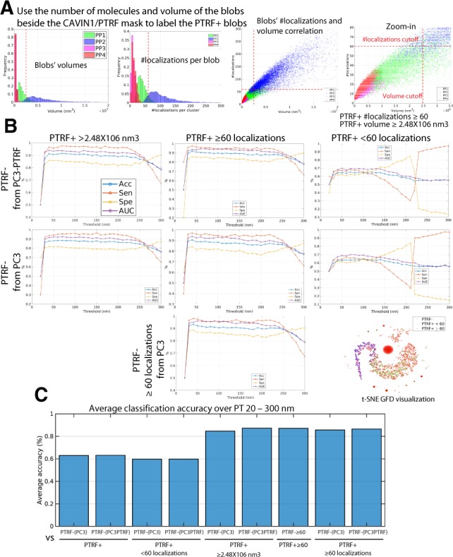
Application of other learned features (number of localizations, volume) to improve blob identification using the CAVIN1/PTRF mask. (A) The volume and number of localizations for the blobs labeled using the unsupervised labeling method (Khater et al., 2018). The linear relationship (with 94% correlation) between the volume and number of localizations features shows that either can be used along with CAVIN1/PTRF mask to identify PTRF+ blobs. (B) Using the CAVIN1/PTRF mask to further label PTRF+ blobs, based on either number of localizations (PTRF+ $\ge 60$ and PTRF+ < 60) or volume (PTRF+ $\ge 2.48\times {10}^6{\text{nm}}^3$ and PTRF+ $<2.48\times {10}^6{\text{nm}}^3$) and then, extracting GFD features for machine learning classification to automatically classify the blobs at various PTs. (C) The bar plot shows average classification Acc of the blobs over the used PTs for the binary classifiers in (B) above. The Number of localizations and volume cut-offs improves blob identification

We then compared classification similarity between the supervised and unsupervised learning approaches (Fig. 6). Caveolae (PP2) showed low classification Acc (i.e. <45%) with the large PTRF+ $\ge 60$ nodes group and high classification with small PTRF+ and PTRF− clusters. Conversely, S2 (PP1), S1B (PP3) and S1A (PP4) scaffolds showed high classification Acc with large PTRF+ clusters and reduced classification Acc with small PTRF+ and PTRF− clusters (Fig. 6A and B). Plotting GFD for each graphlet shows excellent matching for caveolae GFD signatures from PP2 and PTRF+ blobs >$2.48\times {10}^6{\text{nm}}^3$ or >60 nodes (Fig. 6C and D). Small PTRF+ blobs (<60 nodes) closely match PTRF− blobs and show significant reduction in one connected and two disconnected graphlets. Similar analysis of the unsupervised learning groups shows that larger hemispherical S2 scaffolds (PP1) are most similar to caveolae (PP2) and that the smaller S1B (PP3) and S1A (PP4) scaffolds most closely match the PTRF− group (Fig. 6C and D).

Fig. 6.

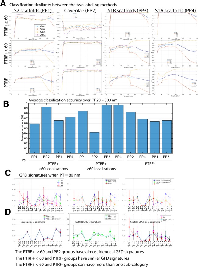
Using GFD biosignatures for machine learning classification of the Cav1 blobs. (A) Identifying the Cav1 domains via classification of all combinations of blob groups using unsupervised learning-based blob labels PP1, PP2, PP3, PP4 or CAVIN1/PTRF mask-based supervised learning PTRF+ $\ge 60$, PTRF+<60, PTRF−. The classification results show similar and dissimilar groups based on extracted GFD features at various PTs. For example, low classification Acc of PP2 and PTRF+$\ge 60$ suggests that the GFD features of these two groups are very similar and represent the same group of Cav1 domains (i.e. caveolae). (B) Bar plot shows average classification Acc of blobs over the used PTs for the binary classifiers in (A) above. (C) GFD signatures for the blobs at PT=80 nm using the different labeling methods. Using either number of localizations or volume cut-offs to label PTRF+ blobs leads to similar GFD biosignatures. (D) Depicting GFD biosignatures for blobs from the various groups shows that the similar Cav1 domains have similar feature trends. For example, PP2 blobs have almost identical features to PTRF+$\ge 60$ and PTRF+$\ge 2.48\times {10}^6{\text{nm}}^3$ and correspond to caveolae. GFD feature trends represent a biosignature for each Cav1 domain

Caveolae show a high frequency of 4-path ($g{4}_6$) graphlets while small scaffolds show increased frequency of 4-clique ($g{4}_1$) and 4-chordal-cycle ($g{4}_2$) at low PTs that increase for all domains with increasing PT in relation to blob size (Fig. 7A). Conversely, 4-node-independent is more frequent in large blobs at low PT and disappears from all blobs at high PT values. This highlights the high interconnectivity of nodes within Cav1 domains (Fig. 7B). Interestingly, all groups show a similar frequency of 4-tailed triangle ($g{4}_3$) at low PT whose decreasing frequency at higher PTs corresponds to blob size. Further, 4-cycle graphlets are absent from all Cav1 domains (Fig. 7A). In contrast, we observe a high frequency ($>60\%$) of 4-node-1-triangle ($g{4}_7$) disconnected and 4-tailed triangle ($g{4}_3$) connected graphlet patterns in all Cav1 domains that vary in proportion to blob size.

Fig. 7.

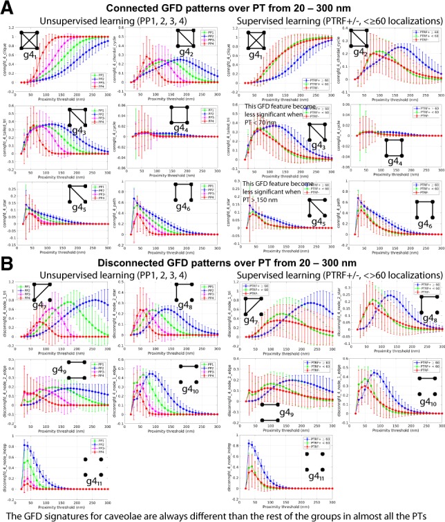
GFD discriminatory features for the different Cav1 blobs over various PTs. The change in GFD features over various PTs using two different labeling strategies for the Cav1 blobs. The mean and standard deviation of (A) connected and (B) disconnected features have different values based on the used PT. Some GFD features are not informative and unchanged with different PTs (e.g. $g{4}_4$). Some features show that the similar groups have the same trends over the different PTs (e.g. PTRF− and PTRF+<60)

4 Discussion

We show here that graphlet analysis of single molecule super-resolution data can identify and discriminate Cav1 domains. Studying the frequencies of the various graphlet patterns in the different Cav1 domains’ networks represent compressed descriptors to training the machine learning approaches to identifying the biological structures automatically and effectively. The different Cav1 domains have distinct GFD patterns and features suggestive of altered molecular stoichiometry within these biological structures. Application of GFD analysis to SMLM data requires reduction of the millions of blinks obtained by SMLM to obtain representative molecular localizations. Each Cav1 molecule can be labeled by multiple primary and secondary antibodies, with the latter carrying multiple fluorophores. To do this, we merge blinks derived from individual Cav1 proteins by iteratively combining blinks within a defined 20 nm distance, generating a predicted Cav1 localization (Khater et al., 2018). Choice of merge threshold will necessarily impact the number of predicted localizations studied and use of a fixed 20 nm threshold will not necessarily take into consideration the reduced axial resolution of cylindrical lens-based 3D SMLM. Nevertheless, application of a 20 nm to the SMLM dataset obtained from PC3-PTRF cells effectively identified and distinguished caveolae from smaller scaffold structures (Khater et al., 2018). Importantly, the caveolae identified showed structural similarities to those predicted by cryoEM (Ludwig et al., 2016; Stoeber et al., 2016).

This study extended that work to include a wide-field mask for CAVIN1/PTRF, a required adaptor for caveolae formation (Hill et al., 2008). The demonstration here that GFD-based machine learning classifies caveolae Cav1 blobs with large (>60 nodes) CAVIN1/PTRF+ blobs confirms that the 3D SMLM Network Analysis pipeline, as applied here, can enable structural analysis of Cav1 domains. The low classification Acc of PTRF+ and PTRF− blobs contrasts the high classification Acc of PP1, PP2, PP3 and PP4 groups. Classification Acc improved upon stratification of the PTRF+ blobs based on size, either number of nodes or volume. This suggests that smaller S1 and/or S2 scaffolds also interact with the wide-field CAVIN1/PTRF mask. While resolution of the wide-field CAVIN1/PTRF mask is significantly reduced relative to the SMLM-characterized Cav1 blobs, these data suggest that CAVIN1/PTRF is not exclusively associated with caveolae, but may also interact with Cav1 scaffolds.

High classification Sen (or high true positive rate) (Figs 3B and 5B) means that the classifier correctly identifies the PTRF+ blobs, while at the same time lower Spe (true negative rate) means that PTRF− blobs are harder to identify and the majority of the mis-classified blobs are from negative blobs. The Spe and Sen show that positive blobs have less mis-predictions. The models with high Sen and low Spe are good for catching actual positive cases.

Machine learning-based classification of the various Cav1 domains with graphlet analysis helped us to: (i) identify the Cav1 domains and draw their biosignatures; and (ii) find the best range of PTs to identify significant molecular interactions (classification loss and mis-prediction is <10%) in each of the Cav1 domains. Classification Acc is reduced at PTs below 50 and above 150 nm due to the less discriminatory GFD features at these ranges of PTs (Supplementary Fig. S1C). This suggests that molecular interaction should not be studied at an arbitrary spatial scale since there is a critical range of spatial distances within which class-specific molecular interaction occurs.

Frequency of some molecular interaction patterns in certain structures distinguishes them from other structures (i.e. every biological structure type has unique patterns of its molecular interactions). For instance, the highly connected 4-clique ($g{4}_1$) and 4-chordal-cycle ($g{4}_2$) GFD patterns (Figs 3A and 7A) have higher frequencies in both S1A and S1B scaffolds compared with S2 scaffold and caveolae. At the same time, the less highly connected 3-star ($g{4}_5$) and 4-path ($g{4}_6$) patterns have lower frequencies in both S1A and S1B scaffolds compared with S2 scaffolds and caveolae. The high frequency of 4-clique ($g{4}_1$) patterns is indicative of saturation of molecular interactions and suggest that S1A and S1B scaffolds contain a higher frequency of stable patterns of strong intermolecular interactions. Indeed, S1A scaffolds correspond to SDS-resistant Cav1 homo-oligomers detected biochemically (Monier et al., 1995; Sargiacomo et al., 1995). Interestingly, the 4-cycle ($g{4}_4$) closed chain pattern is essentially absent in all Cav1 domains at all PTs (Fig. 7A) suggesting that a planar square pattern of molecular interaction is not associated with Cav1 domains. This is consistent with the reported presence of regular hexagonal profiles in the polyhedral cage of the Cav1 caveolar coat observed by cryoEM (Ludwig et al., 2016).

The t-SNE visualization in Figures 3A and 5B shows that the projected GFD features depict more clustering behavior amongst the blobs from similar classes. The separation of the blob classes in Figure 3A is better than Figure 5B and much better than Figure 4B. Also, it shows that the clustering behavior of the PTRF+ blobs is much clearer after stratification based on the number of molecular localizations (Fig. 5B). The overlap of the GFD features for some of the PTRF+ $\ge 60$ blobs with some of the PTRF− blobs may be due to the commonality of GFD features that appear in blobs from the different Cav1 domains.

This study represents the novel application of graphlet analysis to point clouds generated from SMLM datasets. Graphlets represent features that can be used to classify biological structures, define biosignatures associated with specific biological structures and identify molecular interaction motifs associated with specific biological structures. Extension of this approach to biological structures other than Cav1 domains is warranted.

References

- Ahmed N.K. et al. (2015) Efficient graphlet counting for large networks. In: 2015 IEEE International Conference on Data Mining (ICDM) pp. 1–10. IEEE.
- Ahmed N.K. et al. (2017) Graphlet decomposition: framework, algorithms, and applications. Knowl. Inf. Syst., 50, 689–722. [Google Scholar]
- Bassett D.S., Sporns O. (2017) Network neuroscience. Nat. Neurosci., 20, 353.. [DOI] [PMC free article] [PubMed] [Google Scholar]
- Benson A.R. et al. (2016) Higher-order organization of complex networks. Science, 353, 163–166. [DOI] [PMC free article] [PubMed] [Google Scholar]
- Bressan M. et al. (2017) Counting graphlets: space vs time. In: Proceedings of the Tenth ACM International Conference on Web Search and Data Mining pp. 557–566. ACM.
- Brown C.J. et al. (2014) Structural network analysis of brain development in young preterm neonates. Neuroimage, 101, 667–680. [DOI] [PubMed] [Google Scholar]
- Costa L.d.F. et al. (2008) Complex networks: the key to systems biology. Genet. Mol. Biol., 31, 591–601. [Google Scholar]
- Dutta A., Sahbi H. (2017) High order stochastic graphlet embedding for graph-based pattern recognition. arXiv 1702, 00156. [Google Scholar]
- Gumhold S. et al. (2001) Feature extraction from point clouds. In: 10th International Meshing Roundtable, Newport Beach, California, USA.
- Hansen C.G. et al. (2013) Deletion of cavin genes reveals tissue-specific mechanisms for morphogenesis of endothelial caveolae. Nat. Commun., 4, 1831.. [DOI] [PMC free article] [PubMed] [Google Scholar]
- Hill M.M. et al. (2008) PTRF-Cavin, a conserved cytoplasmic protein required for caveola formation and function. Cell, 132, 113–124. [DOI] [PMC free article] [PubMed] [Google Scholar]
- Hočevar T., Demšar J. (2014) A combinatorial approach to graphlet counting. Bioinformatics, 30, 559–565. [DOI] [PubMed] [Google Scholar]
- Khater I.M. et al. (2018) Super resolution network analysis defines the molecular architecture of caveolae and caveolin-1 scaffolds. Sci. Rep., 8, 9009.. [DOI] [PMC free article] [PubMed] [Google Scholar]
- Kollias G. et al. (2012) Network similarity decomposition (NSD): a fast and scalable approach to network alignment. IEEE Trans. Knowl. Data Eng., 24, 2232–2243. [Google Scholar]
- Krivitsky P.N. et al. (2009) Representing degree distributions, clustering, and homophily in social networks with latent cluster random effects models. Soc. Networks, 31, 204–213. [DOI] [PMC free article] [PubMed] [Google Scholar]
- Liu L., Pilch P.F. (2008) A critical role of cavin (polymerase I and transcript release factor) in caveolae formation and organization. J. Biol. Chem., 283, 4314–4322. [DOI] [PubMed] [Google Scholar]
- Ludwig A. et al. (2016) Architecture of the caveolar coat complex. J. Cell Sci., 129, 3077–3083. [DOI] [PMC free article] [PubMed] [Google Scholar]
- Maaten L.v.d., Hinton G. (2008) Visualizing data using t-SNE. J. Mach. Learn. Res., 9, 2579–2605. [Google Scholar]
- Marcus D., Shavitt Y. (2012) Rage–a rapid graphlet enumerator for large networks. Comput. Netw., 56, 810–819. [Google Scholar]
- Milo R. et al. (2002) Network motifs: simple building blocks of complex networks. Science, 298, 824–827. [DOI] [PubMed] [Google Scholar]
- Monier S. et al. (1995) VIP21-caveolin, a membrane protein constituent of the caveolar coat, oligomerizes in vivo and in vitro. Mol. Biol. Cell, 6, 911–927. [DOI] [PMC free article] [PubMed] [Google Scholar]
- Newman M.E. (2003) The structure and function of complex networks. SIAM Rev., 45, 167–256. [Google Scholar]
- Pržulj N. (2007) Biological network comparison using graphlet degree distribution. Bioinformatics, 23, e177–e183. [DOI] [PubMed] [Google Scholar]
- Pržulj N. et al. (2004) Modeling interactome: scale-free or geometric? Bioinformatics, 20, 3508–3515. [DOI] [PubMed] [Google Scholar]
- Qi C.R. et al. (2017) PointNet: deep learning on point sets for 3D classification and segmentation. In: Proceedings of Computer Vision and Pattern Recognition (CVPR), Vol. 1, IEEE, p.4. [Google Scholar]
- Sargiacomo M. et al. (1995) Oligomeric structure of caveolin: implications for caveolae membrane organization. Proc. Natl. Acad. Sci. USA, 92, 9407–9411. [DOI] [PMC free article] [PubMed] [Google Scholar]
- Shervashidze N. et al. (2009) Efficient graphlet kernels for large graph comparison. In: Artificial Intelligence and Statistics pp. 488–495.
- Shin K. et al. (2016) CoreScope: graph mining using k-core analysis–patterns, anomalies and algorithms. In: 2016 IEEE 16th International Conference on Data Mining (ICDM) pp. 469–478. IEEE.
- Stoeber M. et al. (2016) Model for the architecture of caveolae based on a flexible, net-like assembly of Cavin1 and Caveolin discs. Proc. Natl. Acad. Sci. USA, 113, E8069–E8078. [DOI] [PMC free article] [PubMed] [Google Scholar]
- Yin H. et al. (2017) Local higher-order graph clustering. In: Proceedings of the 23rd ACM SIGKDD International Conference on Knowledge Discovery and Data Mining pp. 555–564. ACM. [DOI] [PMC free article] [PubMed]
- Zhang L. et al. (2013) Discovering discriminative graphlets for aerial image categories recognition. IEEE Trans. Image Process., 22, 5071–5084. [DOI] [PubMed] [Google Scholar]
- Zitnik M., Leskovec J. (2017) Predicting multicellular function through multi-layer tissue networks. Bioinformatics, 33, i190–i198. [DOI] [PMC free article] [PubMed] [Google Scholar]
Associated Data
This section collects any data citations, data availability statements, or supplementary materials included in this article.