MTBI Identification From Diffusion MR Images Using Bag of Adversarial Visual Features

Abstract

In this work, we propose bag of adversarial features (BAF) for identifying mild traumatic brain injury (MTBI) patients from their diffusion magnetic resonance images (MRI) (obtained within one month of injury) by incorporating un-supervised feature learning techniques. MTBI is a growing public health problem with an estimated incidence of over 1.7 million people annually in US. Diagnosis is based on clinical history and symptoms, and accurate, concrete measures of injury are lacking. Unlike most of previous works, which use hand-crafted features extracted from different parts of brain for MTBI classification, we employ feature learning algorithms to learn more discriminative representation for this task. A major challenge in this field thus far is the relatively small number of subjects available for training. This makes it difficult to use an end-to-end convolutional neural network to directly classify a subject from MR images. To overcome this challenge, we first apply an adversarial auto-encoder (with convolutional structure) to learn patch-level features, from overlapping image patches extracted from different brain regions. We then aggregate these features through a bag-of-word approach. We perform an extensive experimental study on a dataset of 227 subjects (including 109 MTBI patients, and 118 age and sex matched healthy controls), and compare the bag-of-deep-features with several previous approaches. Our experimental results show that the BAF significantly outperforms earlier works relying on the mean values of MR metrics in selected brain regions.

I. Introduction

Mild traumatic brain injury (MTBI) is a significant public health problem, which can lead to a variety of problems including persistent headache, memory and attention deficits, as well as behavioral symptoms. There is public concern not only regarding civilian head trauma, but sport-related, and military-related brain injuries [1]. Up to 20–30% of patients with MTBI develop persistent symptoms months to years after the initial injury [2], [3]. Good qualitative methods to detect MTBI are needed for early triage of patients, believed to improve outcome [4].

The exploration of non-invasive methodologies for the detection of brain injury using diffusion MRI is extremely promising in the study of MTBI: e.g., diffusion tensor imaging (DTI) shows areas of abnormal fractional anisotropy (FA) [6]-[7] and mean diffusivity (MD) [8] in white matter (WM); and diffusion kurtosis imaging (DKI) shows altered mean kurtosis (MK) within the thalamus in MTBI [9]-[10]. In addition to these conventional measurements, more recently, white matter tract integrity (WMTI) metrics [11] derived from multi-shell diffusion imaging have been proposed to describe microstructural characteristics in intra- and extra-axonal environments of WM, showing reduced intra-axonal diffusivity (Daxon) in the splenium in MTBI [5]. Recently, there are new approaches incorporating machine learning algorithm on MR images for MTBI identification and prediction [12]-[15]. In spite of the encouraging results, the features used in those works are mainly hand-crafted and may not be the most discriminative features for this task (e.g., mean).

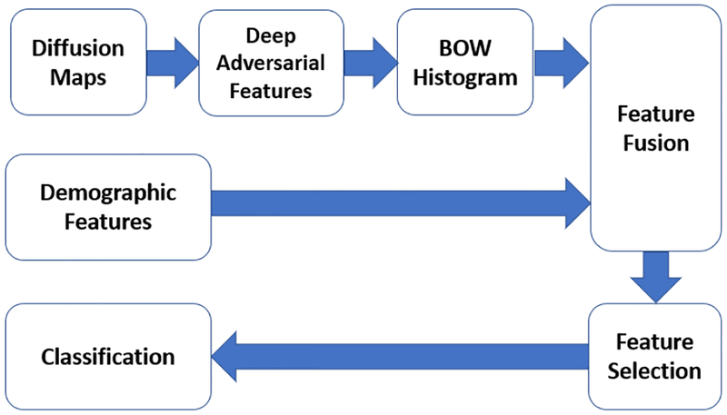
In this work, we propose a machine learning framework to classify MTBI patients from controls using features extracted from diffusion MRI, particularly in the thalamus, and the splenium of the corpus callosum (sCC), two areas that have been highly implicated in this disorder based on previous works [16]-[17]. The main challenge for using a machine learning approach is that, as many other medical image analysis tasks, we have a relatively small (in machine learning sense) dataset of 227 subjects, and each sample has a very high dimensional raw representation (multiple 3D volumes). Therefore, it is not feasible to directly train a classification network on such datasets. To overcome this issue, we propose to learn features from local patches extracted from thalamic and splenial regions-of-interest (ROIs) using a deep adversarial auto-encoder to learn patch level features in an unsupervised fashion, and then aggregate the features from different patches through a bag of word representation. Finally, feature selection followed by a classification algorithm is performed to identify MTBI patients. The block diagram of the overall algorithm is shown in Fig. 1. This approach provides a powerful scheme to learn a global representation by aggregating deep features from local regions, and will be a useful approach in cases where there may be a limited number of samples but high dimensional input data (e.g. MRI).

Fig. 1:

The block-diagram of the proposed MTBI identification algorithm

The remaining parts of the paper are organized as follows. Section II provides an overview of previous works on MTBI detection using MR imaging. Section III describes the details of the proposed framework. The experimental studies and comparison are provided in Section IV. Summary and conclusion are stated in Section V.

II. Previous Works

Diffusion MRI is one of the most promising imaging techniques to detect in vivo injury in patients with MTBI. While many of the studies performed over the past decade show group differences between control subjects and MTBI, the consensus report from the American College of Radiology in 2016, cited the utility of these techniques applied to individual subjects as remaining limited [18].

A small number of studies have used machine learning frameworks applied to imaging to identify patients with MTBI.

Lui et al [12] proposed a machine learning framework based on 15 features, including 2 general demographic features, 3 global brain volumetric features, and 10 regional brain MRI metrics based on previously demonstrated differences between MTBI and control cohorts. Mean value of various metrics in different regions are used as the imaging features in their work. They used Minimum Redundancy and Maximum Relevance (MRMR) for feature selection, followed by a classification algorithm to identify the patients. They evaluated their model on a dataset of 48 subjects, and showed they are able to identify the MTBI patients with reasonably good accuracy using cross-validation sense.

In [13], Vergara et al investigated the use of resting state functional network connectivity (rsFNC) for MTBI identification, and did a comparison with diffusion MRI results on the same cohort. Features based on rsFNC were obtained through group independent component analysis and correlation between pairs of resting state networks. Features from diffusion MRI were obtained using all voxels, the enhanced Z-score micro-structural assessment for pathology, and the distribution corrected Z-score. Linear support vector machine [19] was used for classification and leave-one-out cross validation was used to validate the performance. They achieved a classification accuracy of 84.1% with rsFNC features, compared to 75.5% with diffusion-MRI features, and 74.5% using both rsFNC and diffusion-MRI features.

In addition Mitra [20] proposed an approach for identifying MTBI based on FA-based altered structural connectivity patterns derived through the network based statistical analysis of structural connectomes generated from TBI and age-matched control groups. Higher order diffusion models were used to map white matter connections between 116 cortical and subcortical regions in this work. Then they performed network-based statistical analysis of the connectivity matrices to identify the network differences between a representative subset of the two groups. They evaluated the performance of their model on a dataset of 179 TBI patients and 146 controls participants, and were able to obtain a mean classification accuracy of 68.16%±1.81% for classifying the TBI patients evaluated on the subset of the participants that was not used for the statistical analysis, in a 10-fold cross-validation framework.

There are several other works using imaging features for MTBI identification. For a detailed explanations we refer the readers to [21]-[24]. While such previous works show promising results to identify MTBI based on various machine learning approaches, they are limited by the size of training data, and the usefulness of the hand-engineered features used in those works.

To overcome the limitation of previous works, we propose a new framework for identifying MTBI patients using imaging features. Instead of directly extracting features from the entire brain or selected regions, we propose to describe each selected region by the distribution of local patch patterns. Specifically, we learn patch level features in an unsupervised fashion and aggregate the features through a bag of words representation. Each patient is described by the bag of words representations derived for different MR metrics and region of interests. Compared to the prior works, we included some newly proposed diffusion features to be better able to identify MTBI.

The present work is a significant extension of our preliminary results presented in [25]-[26]. Firstly, the present work differs from those in [25]-[26] in the way the visual features are constructed to derive the visual words. In [25], we directly use the raw image patch as the visual features; and in [26], we use an autoencoder to learn features for image patches. In this paper, we further improve beyond [26] by using an adversarial autoencoder and show that it can significantly improve the classification accuracy over those approaches in [25]-[26]. Secondly, we have doubled the number of human subjects in our analysis, which enabled us to conduct more comprehensive performance evaluation, including evaluation on an independent held-out set. Finally, we proposed novel visualization of visual words in the brain (Figs. 11–12) to help the readers understand the bag of words representation.

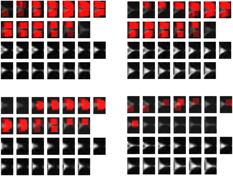
Fig. 11:

Localization heatmaps corresponding to a chosen word in thalamus and MD metric. The figures in top row denote the heatmaps for two patient subjects, and the heatmaps in bottom row denotes the heatmaps for two controls. In each figure, the first two rows denote the location of chosen words in different parts of 13 thalamus slices, and the next two rows denote the actual MD metrics in thalamus for those subjects.

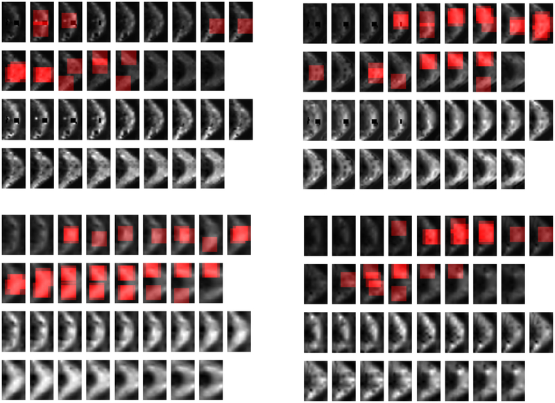
Fig. 12:

Localization heatmaps corresponding to a chosen word in sCC and RK metric. The figures in top row denote the heatmaps for two patient subjects, and the heatmaps in bottom row denotes the heatmaps for two controls. In each figure, the first two rows denote the location of chosen words in different parts of 13 thalamus slices, and the next two rows denote the actual MD metrics in thalamus for those subjects.

III. The Proposed Framework

In this work we propose a machine learning framework for MTBI identification, which relies on the imaging and demographics features. Based on previous studies [5], [9], [27], showing abnormal or altered diffusion values in MTBI, 9 diffusion features were selected: 1) 2 features (fractional anisotropy [FA], mean diffusivity [MD]) from diffusion tensor imaging (DTI) [28], 2) 3 features (mean kurtosis [MK], axial kurtosis [AK], radial kurtosis [RK]) from diffusion kurtosis imaging (DKI) [29], 3) 4 features (axonal water fraction [AWF], intra-axonal diffusivity [DA], extra-axonal axial diffusivity [De-par], extra-axonal radial diffusivity [De-perp]) from white matter tract integrity (WMTI) modeling. These metrics are summarized in Table I.

TABLE I:

MRI metrics description

Diffusion Imaging Features	Description
FA	Fractional Anisotropy
MD	Mean Diffusion
MK, AK, RK	Mean/Axial/Radial Kurtosis
AWF	Axonal Water Fraction
DA	Intra-axonal diffusivity
De-par	Extra-axonal axial diffusivity
De-perp	Extra-axonal radial diffusivity

Specially, this work includes WMTI features that have been proposed to describe microstructural characteristics in intraand extra-axonal environments of white matter, derived from an white matter modeling [11]. Since the WMTI model is designed for single orientation fiber bundles (i.e, highly aligned white matter regions), WMTI features should be applied only for white matter regions, not for thalamus. Thus, for thalamus regions, we use only 5 diffusion features (DTI and DKI) in this study.

Now we need to extract some image descriptors (features) from the images above. Many of the previous works used hand-crafted features for image representation, but since it is not clear beforehand which imaging features are the best for MTBI identification, we propose to learn the feature representation from MR images using a deep learning framework. Because of the limitation of the number of samples, it is not possible to train a deep convolutional network to directly classify the an entire brain image volume. To tackle this problem, and also based on the assumption that MTBI may impact only certain regions in the brain, we propose to represent each brain region by a bag of words (BoW) representation, which is the histogram of different representative patch-level patterns. By looking at 16×16 patches from thalamus and sCC we get around 454 patches from each subject, which results in more than 100k image patches. Since we cannot infer patch level labels from subject label, we should use unsupervised feature learning schemes. We use a recent kind of auto-encoder models, called adversarial auto-encoder, to learn discriminative patch level representations. The detail of feature extraction and bag of word approach are explained in Section III.A and III.B.

A. Adversarial Auto-Encoder for Patch Feature Learning

There have been a lot of studies in image processing and computer vision to design features for various applications. For patch level description, various ”hand-crafted” features have been developed, such as scale invariant feature transform (SIFT), histogram of oriented gradients (HOG), and local binary pattern (LBP) [30]-[33]. Although these features perform well for some applications, there are not the best we could do in many cases. To derive a (more) optimum set of feature for any task, one can use machine learning techniques to learn the representation. Convolutional neural networks are one of the most successful models used for image classification and analysis that jointly learn features and perform classification, and have been used for a wide range of applications from image classification and segmentation, to automatic image captioning [34]-[37].

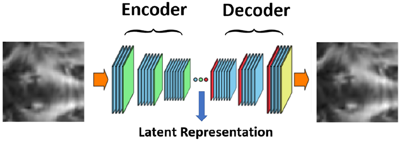
The challenge in our problem is that we do not have patch level classification labels, as we cannot assume all patches from a MTBI subject will be “abnormal”. In order to learn patch-level features without having labels, we employ adversarial auto-encoder [38], an unsupervised feature learning approach. Adversarial auto-encoder is similar to the regular auto-encoder, in that they both receive an image as the input and perform multiple “convolution+nonlinearity+downsampling” layers to encode the image into some latent features, and then use these features to reconstruct the original image through deconvolution. By doing so, the network is forced to learn some representative information that is sufficient to recover the original image. The overall architecture of a regular auto-encoder is shown in Figure 2. It can be seen that the network consists of two main parts, an encoder and a decoder [39]-[40]. In our work we apply the auto-encoder at the patch level. After training this model, the latent representation in the mid-layer is used as patch feature representation.

Fig. 2:

The block-diagram of an example convolutional auto-encoder

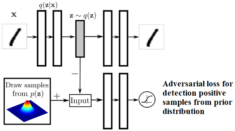
Adversarial auto-encoder has one more component, by which it enforces some prior distribution on the latent representation. As a result, the decoder of the adversarial auto-encoder learns a generative model which maps the imposed prior to the data distribution. The block diagram of an adversarial auto-encoder is shown in Fig 3.

Fig. 3:

Block-diagram adversarial auto-encoder, courtesy of Makhzani [38]

As we can see, there is an discriminator network which classifies whether the latent representation of a given sample comes from a prior distribution (Gaussian in our work) or not. Adding this adversarial regularization guides the auto-encoder to generate latent features with a target distribution.

To train the adversarial auto-encoder, we minimize the loss function in Eq (1) over the training samples. Note that this loss function consists of two terms, one term describes the reconstruction error, and another one the discriminator loss. We use the mean square error for the reconstruction loss, and binary cross entropy for the adversarial loss. The parameter λ is a scalar which determines the relative importance of these two terms, and can be tuned over a validation set. Here X and W denote the training samples, and the model parameters respectively. One can train this model (find the parameters’ values, W) by stochastic gradient descent, which minimizes this loss function over different batches (a subset of the entire samples) of training samples.

$${\mathcal{L}}_{AAE}(X;W)={\mathcal{L}}_{Rec}(X;W)+\lambda {\mathcal{L}}_{Adv}(X;W)$$ (1)

In our study, we train one auto-encoder model for each metric (such as FA, MK, RK, etc.). Therefore we have multiple networks, where each one extracts the features from a specific metric (and both regions). In a preliminary study, we also investigated on training a single model which can jointly learn the feature from all different metrics, but it turns out it performs slightly worse than the current scenario. We will provide the comparison between using adversarial auto-encoder for feature learning, with convolutional auto-encoder, and also with directly using raw voxel values.

B. Bag of Visual Words

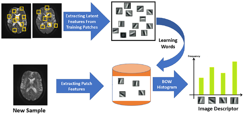
After extraction of the patch-level features, we need to aggregate these features into a global representation for an entire brain volume. One simple way could be to get the average representation of patch features as the overall feature. But this simple approach can lose a lot of information. Instead, we use the bag of words (BoW) representation [41] to describe each brain region, which calculates the histogram of representative patterns (or visual words) over all patches in this region. Bag of visual words is a popular approach in computer vision, and is used for various applications [42]-[43]. The idea of bag of visual words in computer vision is inspired by bag of word representation in text analysis, where a document is represented as a histogram of words, and those histograms are used to analyze the text documents. Since there is no intrinsic words defined for images, we need to first create the visual words. To find the visual words, we can apply a clustering algorithm (e.g. k-means clustering) to the patch features obtained from all training patches. Given the MR images of a subject, we extract overlapping patches from two designated brain regions (thalamus and sCC). We then describe a brain region as a histogram of different visual words among all patches in this region. To be more specific about our work, we extract overlapping patches of 16×16 (with stride of 3) from thalamus and sCC (which resulting in a total of 454 patches for each subject). Therefore in total we get around 103k patches. The block diagram of the BoW approach is shown in Figure 4.

Fig. 4:

The block-diagram of the proposed BoW approach

C. Feature Selection and Classification

After deriving adversarial features for patches from diffusion MR images, we will get a feature vector per metric and region. We concatenate the features from different metrics and regions, with demographic features, to form the final feature vector. We then perform feature selection to minimize the risk of over-fitting before classification [44]-[45]. Various feature selection algorithms are tried, such as greedy forward selection, max-relevance and min-redundancy (MRMR) [46] and max correlation, and it turns out that the greedy forward feature selection works best for our problem. This approach selects the best features one at a time with a given classifier, through a cross-validation approach. Assuming S_k denotes the best subset of features of size k, the (k + 1)-th feature is selected as the one which results in the highest cross-validation accuracy rate along with the features already chosen (in S_k). One can stop adding features, either by setting a maximum size for the feature set, or when adding more features does not increase the accuracy rate. For classification, support vector machine is used in this work (which was shown to perform slightly better than other options such as neural network, and random forest). SVM has two main parameters, C and gamma, where C denotes the penalty parameter for the error term, and gamma denotes the Kernel coefficient. These parameters are tuned by doing a grid search over validation set.

The summary of our validation approach for feature selection is provided here:

• Divide the dataset into training and heldout.

• For each pair of C and gamma:

• Create 100 different training and validation split (using different shuffling) from the original training set.

• Apply the forward feature selection algorithm to select the best subset of features of size N_max, based on average validation error on those 100 splits.

• Select the subset of features, and C_opt and gamma_opt associated with the highest validation accuracy among all possible choices of C and gamma.

• Train a model on the initial training set, using the selected subset of features, and C_opt and gamma_opt, and evaluate the accuracy on the heldout samples.

IV. Experimental Results

We evaluate the performance of the proposed approach on our dataset of 227 subjects. This dataset contains 109 MTBI subjects between 18 and 64 years old, within 1 month of MTBI as defined by the American College of Rehabilitation Medicine (ACRM) criteria for head injury, and 118 healthy age and sex-matched controls. The study is performed under institutional review board (IRB) compliance for human subjects research. Imaging was performed on a 3.0 Tesla Siemens Tim Trio and Skyra scanners including multi-shell diffusion MRI at b-values of 1000 and 2000 s/mm2 at isotropic 2.5mm image resolution.

In-house image processing software developed in MATLAB R2017b was used to calculate 11 diffusion maps including DTI, DKI and WMTI metrics. All diffusion maps in subject space are registered to the Montreal Neurological Institute (MNI) standard template space, by using each subjects fractional anisotropy (FA) image. The regions of thalamus and sCC were extracted from the MNI template and were modified if needed.

We applied BoW approach on three sets of patch-level features, raw voxel values, features generated by a trained convolutional auto-encoder, and features generated by adversarial auto-encoder. The statistical features from each region for each MR metric consists of 5 different statistics including mean, standard deviation, third and fourth moments, and finally entropy of voxel values in that region.

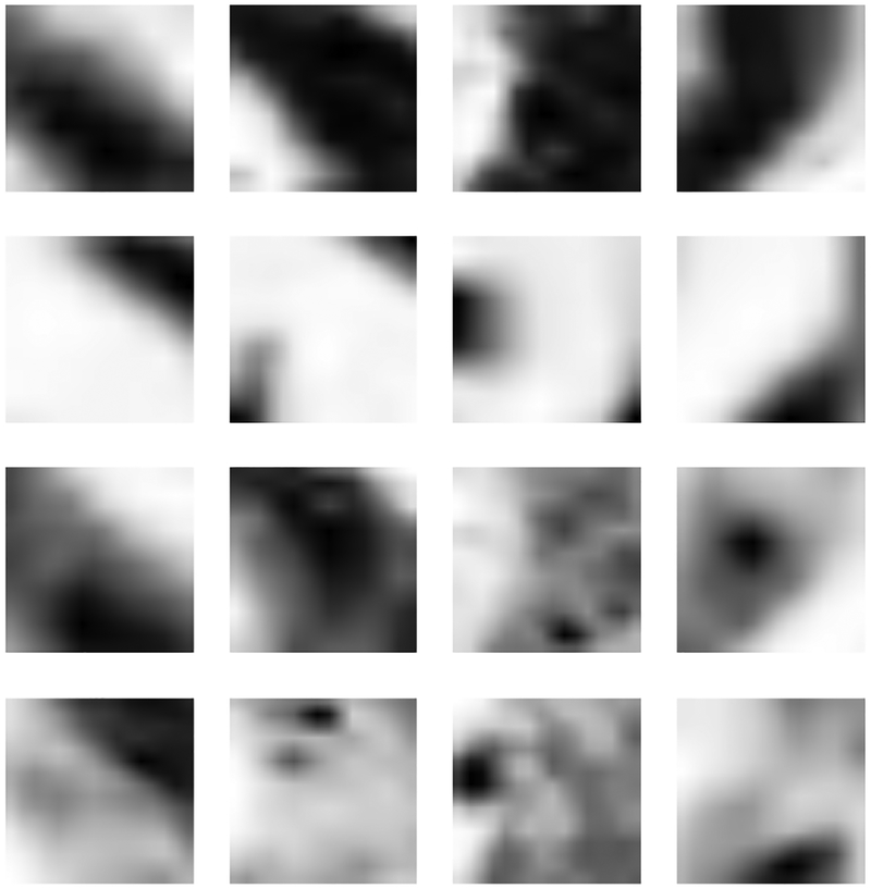
In order to have sense of how patches of different metrics look, some of the sample patches of 16×16 from various metrics are shown in Figure 5.

Fig. 5:

The patches in the first, second, third and fourth rows denote some of the sample patches from FA, MD, Depar and MK metrics.

For the convolutional autoencoder, the encoder and decoder each have 4 layers, and the kernel size is always set to (3,3). The latent feature dimension is 32 for the networks which are trained on individual metrics. To train the model, we use one third of all patches, which is around 34k samples. The batch size is set to 500, and the model is trained for 10 epochs. We use ADAM optimizer to optimize the cost function, with a learning rate of 0.0003. The learnt auto-encoder is then used to generate latent features on each overlapping patch in the training images. The resulting features are further clustered to N words using K-means clustering. N was varied among 20, 30, and 40. Each MR metric in each region is represented by a histogram of dimension N. We used Tensorflow package to train the convolutional-autoencoder model.

For the adversarial auto-encoder, both encoder and decoder networks contain 4 layers (2 ”convolution+nonlinearity+pooling” and 2 fully-connected layers), and the discriminator network contains three fully connected layers, to predict whether a latent representation is coming from a prior distribution or not. The dimension of the latent representation is set to 32 in this case, and the prior distribution of the latent samples is set to be Gaussian. The learning rate during the update of generative and discriminative networks are set to 0.0006 and 0.0008 respectively. Pytorch is used to train the adversarial auto-encoder.

For SVM, we use radial basis function (RBF) kernel. The hyper-parameters of SVM model (kernel width gamma, and the mis-classification penalty weight, C) are tuned based on a validation set of 45 subjects. It is worth to mention that, we normalize all features before feeding as the input to SVM, by making them zero-mean and unit-variance. The SVM module in Scikit-learn package in Python is used to implement SVM algorithm.

A. Classification Accuracies of Different Features

In the first experiment, we compare the performance of the proposed bag-of-adversarial-features with global statistical features, BoW feature derived from convolutional auto-encoder [26], and BoW derived from raw voxel values [25].

In each case (except for the case with statistical features), a histogram of 20-dimensional is derived for each metric in each of thalamus and sCC regions. Then these histograms are concatenated to form the initial image feature, resulting in a 280 dimensional vector, given that there are 9 MR metrics (AWF, DA, De_par, De_perp, FA, MD, AK, MK, RK) in sCC, and 5 MR metrics in thalamus (FA, MD, AK, MK, RK). Together with additional 2 demographic features (age and sex), the total feature dimension is 282.

To perform feature selection and evaluate the model performance, we use a cross validation approach, where each time we randomly take 20% of the samples for validation, and the rest for training. We repeat this procedure 100 times (to decrease sampling bias), and report the average validation error as the model performance.

To have a better generalization accuracy analysis, once the features are chosen, we divide the dataset into three sets, training, validation, and heldout samples, where we train the model on the training set and find the optimum values of the SVM hyper-parameters using the validation set, and evaluate the model performance on the heldout set. In each run, we randomly pick 45 samples out of the entire 227 samples as the heldout set. We then run cross validations 100 times within the remaining data (using 137 samples for training and 45 samples for validation), to generate 100 models, and use the ensemble of 100 models to make prediction on the held-out set and calculate the classification accuracy. We repeat this 4 times, each time with a different set of 45 heldout samples chosen randomly and report the average accuracy. We also calculate the 95% confidence interval of different models accuracies to assess the statistical significance of the proposed model gain. The average accuracies, along with the 95% confidence interval, for the validation and heldout sets for four different approaches are given in Table II. The results reported here use first 10 chosen features for each method. As we can see from this table, the prediction accuracy of the proposed framework is around 2% higher than other features, based on 95% confidence interval, which shows a reasonable improvement. One reason that adversarial features are better than the convolutional features could be that by regularizing the latent representations to be drawn from a prior distribution, it is much easier for the network to converge. Interestingly enough, the heldout accuracies are close to validation accuracies, which could be a good indicator of the generalizability of the proposed features.

TABLE II:

Performance comparison of different approaches using 16×16 patches

The Algorithm	Classification Rate on Validation Set	Classification Rate on Heldout Set
The selected subset of statistical features [25]	78±1.1%	76.6±1.1%
BoW on raw patches with 20D histograms [25]	80.9±1.1%	79.9±1.1%
The Convlutional-BoW with 20D histograms [26]	81.2±1.1%	79.9±1.1%
The proposed Adversarial-BoW (20D histograms)	84.2±1%	83.8±1%

To evaluate the robustness of the model predictions for heldout samples, we evaluated the standard deviation (std) of prediction accuracy over these 100 ensemble predictors. The standard deviations, and 95% confidence interval of different feature sets are shown in Table III. As we can see from this table, the standard variation of all models are relatively small, which is a good indicator of generalization.

TABLE III:

Analysis of mean, standard deviation, and 95% confidence interval of heldout accuracy of different approaches using 16×16 patches

The Algorithm	Classification Rate Mean	Classification Rate STD	The 95% confidence interval
The selected subset of statistical features [25]	76.6%	3.05%	76±1.1%
BoW on raw patches with 20D histograms [25]	79.9%	3.67%	79.9±1.1%
The Convlutional-BoW with 20D histograms [26]	79.9%	3.08%	79.9±1.1%
The proposed Adversarial-BoW (20D histograms)	83.8%	2.85%	83.8±1%

B. Selected Features

With forward feature selection using the SVM classifier, the optimal feature subsets (with maximum feature number set at 10) chosen from different features extraction algorithms are listed in the Table IV. It is worth mentioning that the chosen features vary between techniques and it is not entirely clear why. Of note, our Adversarial BoW technique selects adversarial visual words from kurtosis measures of the thalamus and axonal diffusion, DA, of the splenium of the corpus callosum, both measures which have previously been implicated in differentiating MTBI patients from controls [5], [47]-[48].

TABLE IV:

Chosen features by different approaches. Note that Thal refers to the thalamus region, and sCC refers to Splenium subregion within Corpus Callosum.

The Algorithm	Chosen Features’ Metric and Region
Statistical features	MD in sCC (mean), FA in sCC (entropy), AK in sCC (mean), FA in Thal (mean), MD in Thal (var), Depar in sCC (entropy), MK in sCC (entropy), AWF in sCC (mean), Deperp in sCC (entropy), MK in Thal (entropy)
Raw-BoW	FA in sCC, MD in Thal, MK in sCC, AK in Thal, MD in sCC, AWF in sCC, AK in Thal, Depar in sCC, AK in sCC, FA in Thal
Conv-BoW	FA in Thal, AK in Thal, Depar in sCC, MK in sCC, RK in sCC, AK in sCC, MD in Thal, RK in sCC, MD in Thal, MD in sCC
Adversarial-BoW	MD in Thal, AK in Thal, RK in sCC, FA in Thal, Deperp in sCC, MD in Thal, DA in sCC, MD in sCC, Deperp in sCC, Depar in sCC

C. Sensitivity, Specificity and ROC Curve Analysis

Besides classification accuracy, we also report the sensitivity and specificity, which are important in the study of medical data analysis. The sensitivity and specificity are defined as in Eq (2), where TP, FP, TN, and FN denote true positive, false positive, true negative, and false negative respectively. In our evaluation, we treat the MTBI subjects as positive.

$$\text{Sensitivity}=\frac{\text{TP}}{\text{TP}+\text{FN}},\text{ Specificity}=\frac{\text{TN}}{\text{TN}+\text{FP}}$$ (2)

The sensitivities and specificities for different features are shown in Table V.

TABLE V:

Sensitivity and specificity of different approaches on validation set

The Algorithm	Sensitivity	Specificity
Statistical	82.8	74.1
Raw-BoW	79.5	82.3
Conv-BoW	80.2	82.1
Adv-BoW	86.1	81.8

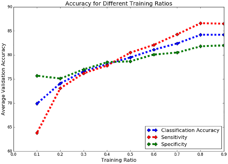
Figure 6 denotes the validation classification accuracies, sensitivities and specificities achieved by different ratios of training samples using adversarial features. We see that using approximately 80% of training samples gives reasonably well validation performance, and we do not gain much by using higher ratios of training samples. Similar trends were observed with other features as well. All other results reported in this paper were using 80% samples for training and 20% for validation, in the cross validation study.

Fig. 6:

The model performance for different training ratios

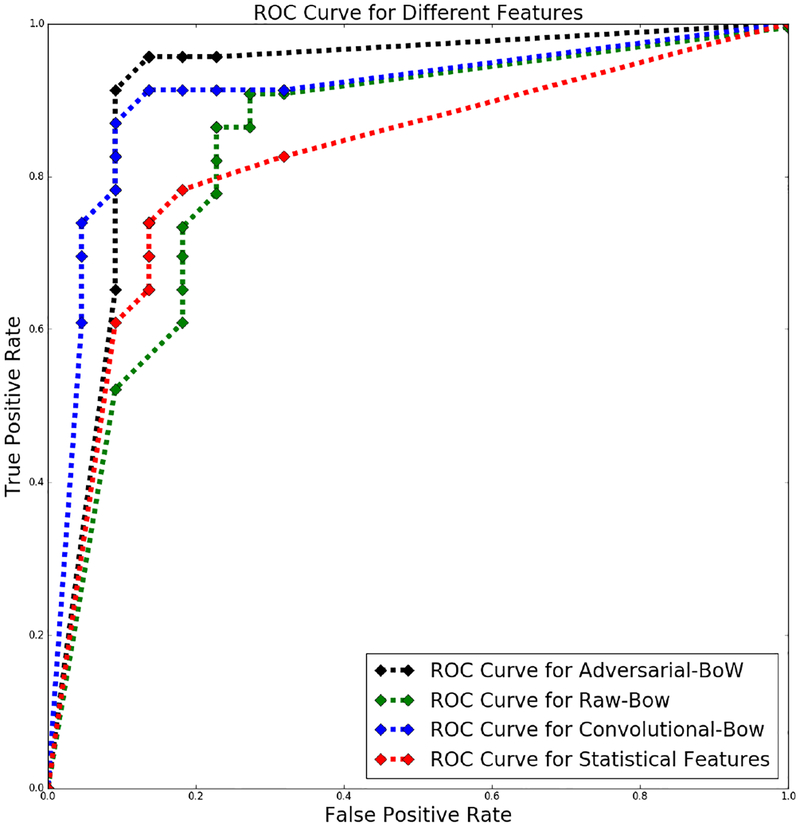
In Figure 7, we present the receiver operating characteristic (ROC) curve for different set of features on heldout samples. ROC curve is a plot which illustrates the diagnostic ability of a binary classifier system as its discrimination threshold is varied. This curve is created by plotting the true positive rate (i.e. sensitivity) against the false positive rate for various threshold settings. Recall that we use the mean prediction of 100 classifiers to predict whether a subject has MTBI. Previously reported results are obtained with a threshold of 0.5 on the mean prediction. The ROC curve is derived by varying the threshold from 0 to 1 with a stepsize of 0.05. As we can see the adversarial and convolutional features provide higher sensitivities under the same false positive rate than the other two methods, and overall have larger areas under the curve (AUCs).

Fig. 7:

The ROC curve for different features

D. Impact of Number of Features and Histogram Dimension

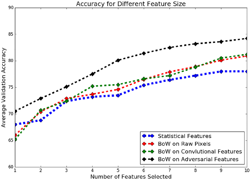
We also studied the classification performance using feature subset of different sizes. These results are shown in Figure 8. We see that with more than 10 features, it is possible to further improve the results slightly, except with the statistical features.

Fig. 8:

The model performance for feature sets of different sizes

In another experiment, we evaluated the impact of histogram dimension on the classification performance. We generated histograms of 10, 20, and 30 dimensions, respectively, for each metric and region, and performed classification. The accuracies and confidence intervals of different histogram dimensions are reported in Table VI. Using 20 dimensional histogram yields the best performance on the held-out set.

TABLE VI:

Impact of the number of clusters (or histogram dimension)

The BoW Histogram Dimension	Classification Rate on Validation Set	Classification Rate on Heldout Set
10	80±1.1%	79.4±1.1%
20	84.2±1%	83.8±1%
30	84.5±1%	82.9±1%

E. The Impact of Patch Dimension

In another experiment, we study the impact of image patch’s dimension, on the final classification performance. Choosing a large patch size, would decrease the number of total patches for each brain image (resulting in a less reliable histogram representations), and choosing a small patch would lead to lack of enough patterns in each patch, resulting in less discriminative histogram representation. We apply our framework on 3 different patch sizes, 8×8, 16×16 and 32×32. Table VII presents the validation and heldout accuracy of this framework using different patch sizes, as well as 95% confidence intervals. As we can the model based on 16×16 patches achieves the highest classification accuracy on the heldout set.

TABLE VII:

Impact of patch dimension on the classification accuracy rate

Patch Dimension	Classification Rate on Validation Set	Classification Rate on Heldout Set
8×8	81.2±1.1%	72.5±1.2%
16×16	80.9±1.1%	79.9±1.1%
32×32	66.1 ±1.3%	60±1.4%

F. The Impact of Feature Selection Approach

There are several ways to perform feature selection for a classification task. Feature selection algorithms are divided into three broad categories: wrapper, filter, embedded. In this work, we relied on greedy forward feature selection, which belongs to the category of wrapper feature selection. One can also try other approaches such as joint feature selection and classification (a kind of embedded algorithm) to simultaneously perform feature selection and classification. L1-SVM is a popular algorithm for joint feature selection and classification. It adds an ${\mathcal{l}}_1$ regularization on the weights, forcing many of them to be zero. In this way, we can treat features with nonzero weights as the selected ones. We start by setting aside a held-out set of the same size. There is a regularization weight, $C_{{\mathcal{l}}_1}$, associated with this term which determines the amount of sparsity. We tried 100 different values for $C_{{\mathcal{l}}_1}$, and selected the $C_{{\mathcal{l}}_1}$ with the highest average validation accuracy across all shufflings and re-train the model using that $C_{{\mathcal{l}}_1}$ on the whole dataset except for the held-out. The classification performance of the ${\mathcal{l}}_1$-SVM model on validation and heldout set is provided in Table VIII. The number of selected features associated with the $C_{{\mathcal{l}}_1}$ value resulting in the highest validation accuracy is 30.

TABLE VIII:

Comparison of performance of different feature selection approaches

Patch Dimension	Classification Rate on Validation Set	Classification Rate on Heldout Set
Forward feature selection	84.2±1%	83.8± 1%
${\mathcal{l}}_1$-SVM based feature selection	69.6± 1.3%	67.5± 1.3%

G. The Impact of Latent Prior Distribution

As mentioned in Section III, one needs to impose some prior distribution on latent variables of adversarial auto-encoder. Gaussian distribution on latent variables, z, is most commonly used and is also adopted in our approach. However, because these latent features are clustered to generate the BoW histograms, it is also natural to explore the use of a Gaussian mixture distribution on the latent variables, and treat each mixture as a visual word cluster. By imposing Gaussian mixture on patch level features, we can follow two different directions for deriving the brain-level features (as histogram of patch-level features):

• Assign the latent representation of each patch to the mixture with the highest likelihood, and derive the histogram. We call this nearest-neighbor clustering approach.

• Assign the latent representation of each patch to different clusters with a weight proportional to the likelihood of each mixture. We call this likelihood clustering approach.

We trained an adversarial auto-encoder with Gaussian mixture prior on our brain patches, and derived the histogram features using both of the above schemes, and performed classification. We have set the number of Gaussian mixtures to 20, so that the brain-level features are 20-dimensional and consistent with our other experiments. Also all Gaussian mixtures are set to be equally likely. The mean of these Gaussians are set as one-hot vectors to ensure equal distance, and their covariance are set to be identical and diagonal so that different dimensions of each Gaussian are i.i.d. The results are summarized in Table IX. We can see that using the Gaussian prior yields better results.

TABLE IX:

The classification results using different distributions on latent variables

Patch Dimension	Validation Classification	Heldout Classification
Gaussian prior with k-means clustering	84.2±1%	83.8±1%
Gaussian mixture prior with nearest neighbor clustering	77.5±1.1%	67.5±1.3%
Gaussian mixture prior with likelihood clustering	75 ±1.2%	70±1.3%

H. Comparison of TBI and Control Histograms

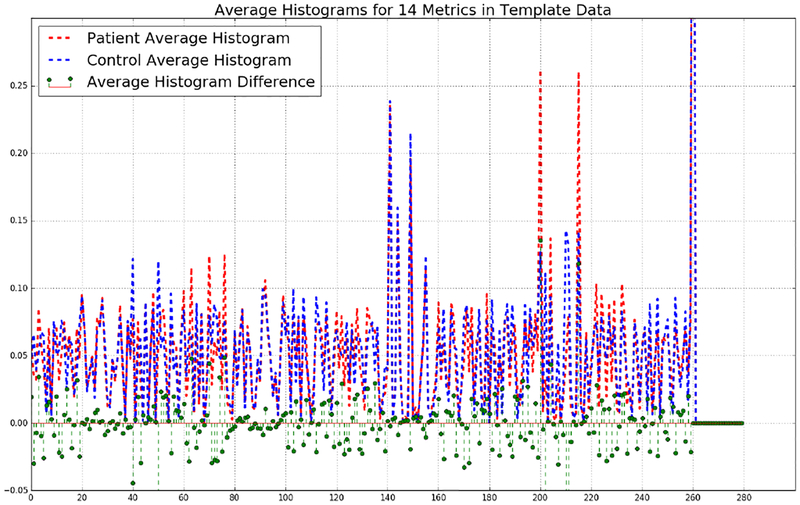
Finally, we present the average histograms of MTBI, and control subjects. These histograms and their difference are shown in Fig 9. As we can see MTBI and control subjects have clear differences in some parts of these representations.

Fig. 9:

Adversarial-BoW histograms of patients and controls

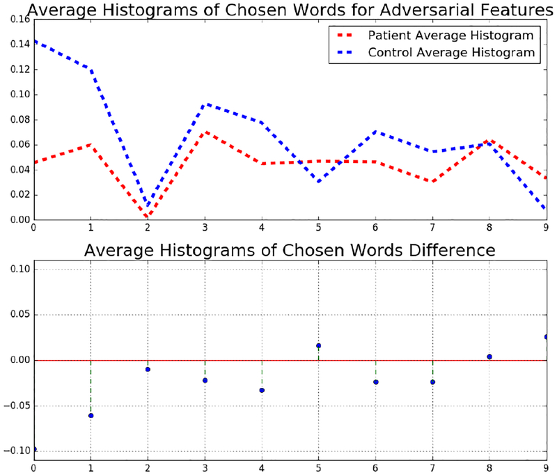
We also find the average histogram over the chosen words for MTBI and control subjects. These histograms are shown in Fig 10. As we can, MTBI and control subjects have clear differences over the chosen words. For example the first two words, are less frequent in patients, than in controls.

Fig. 10:

Adversarial-BoW histograms over the chosen words

I. Localization of Potential Impacted Regions

We also tried to localize the chosen words within the brain. To do so, each time we focus on one of the words chosen by the proposed classification algorithm, and then go over all patches of 16×16 in thalamus and sCC (by shifting the patches with some stride) to see if they are quantized to the chosen word. If so, we increment by one the voxel values in that patch to active regions, and repeat this procedure for the remaining patches. Here, we provide the heatmaps of two patients and two control subjects for two chosen words. These heatmaps are illustrated in Fig 11–12. As we can see from Fig 11, this word is much more frequent in patient subjects, than in controls. It could imply that, this word has some MTBI related information. Note that, for each case, the top two rows denote the heatmap of a specific word over different slices, and the bottom two rows denote the actual metric of those slices. We intentionally increased the contrast of the actual metrics in the bottom to row, for better illustration.

V. Conclusion

In this work, we propose an unsupervised learning framework for MTBI identification from diffusion MR images using a dataset of 227 subjects. We first learn a good representation of each brain regions, by employing a deep unsupervised learning approach that learns feature representation for image patches, followed by aggregating patch level features using bag of word representation to form the overall image feature. These features are used along with age and gender as the final feature vector. Then greedy forward feature selection is performed to find the best feature subset, followed by SVM to perform classification. Through experimental studies, we show that by learning deep visual features at the patch level, we obtain significant gain over using mean values of MR metrics in brain regions. The performance is also improved over the approach where the visual words are determined based on the raw image patch representation. Furthermore, we found that the features learnt with an adversarial autoencoder are more powerful than a non-adversarial autoencoder. This methodology may be of particular use for learning features from datasets with relatively small number of samples, as can be encountered in some medical image analysis studies. The learned features could also be used for tasks other than classification such as long-term outcome prediction.

References

- [1].Faul MLW, Wald MM, Coronado VG, “Traumatic Brain Injury in the United States: Emergency Department Visits, Hospitalizations and Deaths”, 2010.
- [2].Voormolen DC, Cnossen MC, Polinder S, Steinbuechel NV, Vos PE, and Haagsma JA, “Divergent classification methods of post-concussion syndrome after mild traumatic brain injury: Prevalence rates, risk factors and functional outcome”, Journal of neurotrauma, 2018. [DOI] [PMC free article] [PubMed] [Google Scholar]
- [3].Roe C, Sveen U, Alvsaker K and Bautz-Holter E “Post-concussion symptoms after mild traumatic brain injury: influence of demographic factors and injury severity in a 1-year cohort study”, Disability and rehabilitation, 31, 1235–1243, 2009. [DOI] [PubMed] [Google Scholar]
- [4].Grossman EJ, Inglese M, Bammer R, “Mild traumatic brain injury: is diffusion imaging ready for primetime in forensic medicine?”, Topics in magnetic resonance imaging: TMRI 216: 379, 2010. [DOI] [PMC free article] [PubMed] [Google Scholar]
- [5].Chung S, Fieremans E, Wang X, Kucukboyaci NE, Morton CJ, Babb J, Amorapanth Prin et al. “White matter tract integrity: an indicator of axonal pathology after mild traumatic brain injury”, Journal of neurotrauma 35, no. 8: 1015–1020, 2018. [DOI] [PMC free article] [PubMed] [Google Scholar]
- [6].Inglese M, Makani S, Johnson G, Cohen BA, Silver JA, Gonen O, and Grossman RI, “Diffuse axonal injury in mild traumatic brain injury: a diffusion tensor imaging study”, Journal of neurosurgery 103, no. 2: 298–303, 2005. [DOI] [PubMed] [Google Scholar]
- [7].Kraus MF, Susmaras T, Caughlin BP, Walker CJ, Sweeney JA, Little DM, “White matter integrity and cognition in chronic traumatic brain injury: a diffusion tensor imaging study”, Brain, 130(10), 2508–2519, 2007. [DOI] [PubMed] [Google Scholar]
- [8].Shenton ME, Hamoda HM, Schneiderman JS, et al. “A review of magnetic resonance imaging and diffusion tensor imaging findings in mild traumatic brain injury”, Brain imaging and behavior 62: 137–192, 2012. [DOI] [PMC free article] [PubMed] [Google Scholar]
- [9].Grossman EJ, Jensen JH, Babb JS, Chen Q, Tabesh A, Fieremans E, Xia D, Inglese M, Grossman RI, “Cognitive impairment in mild traumatic brain injury: a longitudinal diffusional kurtosis and perfusion imaging study”, American Journal of Neuroradiology,34(5):951–7, 2013. [DOI] [PMC free article] [PubMed] [Google Scholar]
- [10].Stokum JA, Sours C, Zhuo J, Kane R, Shanmuganathan K, and Gullapalli RP, “A longitudinal evaluation of diffusion kurtosis imaging in patients with mild traumatic brain injury”, Brain injury 29, no. 1: 47–57, 2015. [DOI] [PubMed] [Google Scholar]
- [11].Fieremans E, Jensen JH, Helpern JA, “White matter characterization with diffusional kurtosis imaging”, Neuroimage, Elsevier, 177–188, 2011. [DOI] [PMC free article] [PubMed] [Google Scholar]
- [12].Lui YW, Xue Y, Kenul D, Ge Y, Grossman RI, Wang Y, “Classification algorithms using multiple MRI features in mild traumatic brain injury”, Neurology 8314: 1235–1240, 2014. [DOI] [PMC free article] [PubMed] [Google Scholar]
- [13].Vergara VM, Mayer AR, Damaraju E, Kiehl KA, Calhoun V, “Detection of mild traumatic brain injury by machine learning classification using resting state functional network connectivity and fractional anisotropy”, Journal of neurotrauma, 2017. [DOI] [PMC free article] [PubMed] [Google Scholar]
- [14].Minaee S, Wang Y, Lui YW, “Prediction of longterm outcome of neuropsychological tests of MTBI patients using imaging features”, Signal Processing in Medicine and Biology Symposium, IEEE, 2013. [Google Scholar]
- [15].Minaee S, Wang Y, Chung S, et al. “A Machine Learning Approach For Identifying Patients with Mild Traumatic Brain Injury Using Diffusion MRI Modeling”, The American Society of Functional Neuro-radiology (ASFNR), 12th Annual Meeting, 2017. [Google Scholar]
- [16].Grossman EJ, Inglese M, “The role of thalamic damage in mild traumatic brain injury”, Journal of neurotrauma, 33(2), pp.163–167, 2016. [DOI] [PMC free article] [PubMed] [Google Scholar]
- [17].Treble A, Hasan KM, Iftikhar A, et al. “Working memory and corpus callosum microstructural integrity after pediatric traumatic brain injury: a diffusion tensor tractography study”, Journal of neurotrauma, 30(19), 1609–1619, 2013. [DOI] [PMC free article] [PubMed] [Google Scholar]
- [18].Carroll LJ, Cassidy JD, Peloso PM, et al. “Prognosis for mild traumatic brain injury: results of the WHO Collaborating Centre Task Force on Mild Traumatic Brain Injury” J Rehabil Med: 84105, 2004. [DOI] [PubMed] [Google Scholar]
- [19].Cortes Corinna, and Vapnik Vladimir. ”Support-vector networks”, Machine learning 203: 273–297, 1995. [Google Scholar]
- [20].Mitra J, Shen K, Ghose S, Bourgeat P, Fripp J, Salvado O, Pannek K, Taylor DJ, Mathias JL, and Rose S, “Statistical machine learning to identify traumatic brain injury (TBI) from structural disconnections of white matter networks”, NeuroImage 129, 247–259, 2016. [DOI] [PubMed] [Google Scholar]
- [21].Shaker M, Erdogmus D, Dy J, Bouix S, “Subject-specific abnormal region detection in traumatic brain injury using sparse model selection on high dimensional diffusion data”, Medical image analysis, 37, 56–65, 2017. [DOI] [PMC free article] [PubMed] [Google Scholar]
- [22].Wu X, Kirov II, Gonen O, Ge Y, Grossman RI, Lui YW, “MR imaging applications in mild traumatic brain injury: an imaging update”, Radiology, 279(3), 693–707, 2016. [DOI] [PMC free article] [PubMed] [Google Scholar]
- [23].Douglas DB, Iv M, Douglas PK, Vos SB, Bammer R, et al. “Diffusion tensor imaging of TBI: potentials and challenges”, Topics in magnetic resonance imaging, 24(5), 241–251, 2015. [DOI] [PMC free article] [PubMed] [Google Scholar]
- [24].Mayer AR, Hanlon FM, Dodd AB, Ling JM, Klimaj SD, Meier TB, “A functional magnetic resonance imaging study of cognitive control and neurosensory deficits in mild traumatic brain injury”, Human brain mapping, 36(11), 4394–4406, 2015. [DOI] [PMC free article] [PubMed] [Google Scholar]
- [25].Minaee S, Wang S, Wang Y, et al. “Identifying Mild Traumatic Brain Injury Patients From MR Images Using Bag of Visual Words”, Signal Processing in Medicine and Biology Symposium, IEEE, 2017. [Google Scholar]
- [26].Minaee S, Wang Y, Choromanska A, Chung S, Wang X, Fieremans E, Flanagan S, Rath J, and Lui YW., “A Deep Unsupervised Learning Approach Toward MTBI Identification Using Diffusion MRI”, The 40th international conference of the IEEE Engineering in Medicine and Biology Society, July 2018. (Accepted). [DOI] [PMC free article] [PubMed] [Google Scholar]
- [27].Mayer AR, Ling J, Mannell MV, Gasparovic C. et al. “A prospective diffusion tensor imaging study in mild traumatic brain injury”, Neurology, 74(8), 643–650, 2010. [DOI] [PMC free article] [PubMed] [Google Scholar]
- [28].Basser Peter J., Mattiello James, and Denis LeBihan. “MR diffusion tensor spectroscopy and imaging”, Biophysical journal, 259–267, 1994. [DOI] [PMC free article] [PubMed] [Google Scholar]
- [29].Jensen JH, Helpern JA, “MRI quantification of nonGaussian water diffusion by kurtosis analysis”, NMR in Biomedicine: 698–710, 2010. [DOI] [PMC free article] [PubMed] [Google Scholar]
- [30].Lowe David, “Distinctive image features from scale-invariant key-points”, International journal of computer vision, 2004. [Google Scholar]
- [31].Bay H, Ess A, Tuytelaars T, Van Gool L, “Surf: Speeded up robust features”, In European conference on computer vision, Springer, 2006. [Google Scholar]
- [32].Dalal N, Triggs B, “Histograms of oriented gradients for human detection”, CVPR, IEEE, 2005. [Google Scholar]
- [33].Guo Z, Zhang L, Zhang D, “A completed modeling of local binary pattern operator for texture classification”, IEEE Transactions on Image Processing 19, no. 6, 2010. [DOI] [PubMed] [Google Scholar]
- [34].Girshick R, Donahue J, Darrell T, Malik J, “Rich feature hierarchies for accurate object detection and semantic segmentation”, CVPR, IEEE, 2014. [DOI] [PubMed] [Google Scholar]
- [35].Ronneberger O, Fischer P, Brox T, “U-net: Convolutional networks for biomedical image segmentation”, In International Conference on Medical image computing and computer-assisted intervention, Springer, 2015. [Google Scholar]
- [36].He K, Zhang X, Ren S, Sun J, “Deep residual learning for image recognition”, In Proceedings of the IEEE conference on computer vision and pattern recognition, 2016. [Google Scholar]
- [37].You Q, Jin H, Wang Z, Fang C, Luo J, “Image captioning with semantic attention”, CVPR, IEEE, 2016. [Google Scholar]
- [38].Makhzani A, Shlens J, Jaitly N, Goodfellow I, Frey B, “Adversarial autoencoders”, arXiv preprint arXiv:1511.05644, 2015. [Google Scholar]
- [39].Masci J, Meier U, Ciresan D, Schmidhuber J, “Stacked convolutional auto-encoders for hierarchical feature extraction”, International Conference on Artificial Neural Networks, 2011. [Google Scholar]
- [40].Leng B, Guo S, Zhang X, Xiong Z, “3D object retrieval with stacked local convolutional auto-encoder”, Signal Processing 112, 2015. [Google Scholar]
- [41].Yang J, Jiang YG, Hauptmann AG, Ngo CW, “Evaluating bag-of-visual-words representations in scene classification”, Proceedings of the international workshop on multimedia information retrieval, ACM, 2007. [Google Scholar]
- [42].Yang Y, Newsam S, “Bag-of-visual-words and spatial extensions for land-use classification”, SIG-SPATIAL international conference on advances in geographic information systems, ACM, 2010. [Google Scholar]
- [43].Peng X, Wang L, Wang X, Qiao Y, “Bag of visual words and fusion methods for action recognition: Comprehensive study and good practice”, Computer Vision and Image Understanding 150: 109–125, 2016. [Google Scholar]
- [44].Guyon I, Elisseeff A, “An introduction to variable and feature selection”, Journal of machine learning research, 3(Mar), 1157–1182, 2003. [Google Scholar]
- [45].Chandrashekar G, Sahin F, “A survey on feature selection methods”, Computers and Electrical Engineering, Elsevier, 2014. [Google Scholar]
- [46].Peng H, Long F, Ding C, “Feature selection based on mutual information criteria of max-dependency, max-relevance, and min-redundancy”, IEEE Transactions on pattern analysis and machine intelligence, 2005. [DOI] [PubMed] [Google Scholar]
- [47].Nss-Schmidt ET, Blicher JU, Eskildsen SF, Tietze A, et al. “Microstructural changes in the thalamus after mild traumatic brain injury: A longitudinal diffusion and mean kurtosis tensor MRI study”, Brain injury, 31(2), 230–236, 2017. [DOI] [PubMed] [Google Scholar]
- [48].Grossman EJ, Ge Y, Jensen JH, Babb JS, et al. “Thalamus and cognitive impairment in mild traumatic brain injury: a diffusional kurtosis imaging study”, Journal of neurotrauma, 29(13), 2318–2327, 2012. [DOI] [PMC free article] [PubMed] [Google Scholar]