Reconstruction of 1,000 projection neurons reveals new cell types and organization of long-range connectivity in the mouse brain

Summary

Neuronal cell types are the nodes of neural circuits that determine the flow of information within the brain. Neuronal morphology, especially the shape of the axonal arbor, provides an essential descriptor of cell type and reveals how individual neurons route their output across the brain. Despite the importance of morphology, few projection neurons in the mouse brain have been reconstructed in their entirety. Here we present a robust and efficient platform for imaging and reconstructing complete neuronal morphologies, including axonal arbors that span substantial portions of the brain. We used this platform to reconstruct more than 1,000 projection neurons in the motor cortex, thalamus, subiculum, and hypothalamus. Together, the reconstructed neurons comprise more than 85 meters of axonal length and are available in a searchable online database. Axonal shapes revealed previously unknown subtypes of projection neurons and suggest organizational principles of long-range connectivity.

In brief

An efficient pipeline for brain-wide imaging and morphological reconstruction of individual neurons, including long-range projection neurons, is presented along with a searchable database containing more than 1,000 fully reconstructed neurons in the mouse neocortex, hippocampus, thalamus and hypothalamus.

Graphical Abstract

Introduction

Mammalian neurons possess extensive axonal arbors that project over long distances (Anderson et al., 2002; Braitenberg and Schüz, 1991; Kita and Kita, 2012; Kuramoto et al., 2013; Wu et al., 2014). These projections dictate how information flows across brain areas. Interareal connections have been studied using tracers that label populations of neurons (Gerfen and Sawchenko, 1984; Hunnicutt et al., 2014; Luppi et al., 1990; Markov et al., 2014; Oh et al., 2014; Veenman et al., 1992; Zingg et al., 2014) or with functional mapping methods at various spatial scales (Greicius et al., 2009; Petreanu et al., 2007). However, these methods average across large groups of neurons, including multiple cell types and obscure fine-scale spatial organization. Mapping brain-wide connectivity at the single neuron level is crucial for delineating cell types and understanding the routing of information flow across brain areas. Very few complete morphological reconstructions of individual neurons are available, especially for long-range projection neurons (Ascoli and Wheeler, 2016; Svoboda, 2011).

Morphological reconstruction is technically challenging because thin axons (diameter: ~100 nm; Anderson et al., 2002; De Paola et al., 2006; Shepherd and Harris, 1998) travel over long distances (centimeters) and across multiple brain regions (Economo et al., 2018; Kita and Kita, 2012; Oh et al., 2014). High-contrast, high-resolution, brain-wide imaging is therefore required to detect and trace axons in their entirety. Earlier studies using imaging in serial sections have reconstructed only small numbers of cells and mostly only partially, because of the difficulty of manual tracing across sections (Blasdel and Lund, 1983; Cowan and Wilson, 1994; Ghosh et al., 2011; Igarashi et al., 2012; Kawaguchi et al., 1990; Kisvárday et al., 1994; Kita and Kita, 2012; Kuramoto et al., 2009, 2015; Oberlaender et al., 2011; Ohno et al., 2012; Parent and Parent, 2006; Ropireddy et al., 2011; Wittner et al., 2007; Wu et al., 2014). Methods in which precisely assembled brain volumes are generated, for example based on block-face imaging, are more efficient for tracing (Economo et al., 2016; Gong et al., 2016; Han et al., 2018; Lin et al., 2018; Portera-Cailliau et al., 2005), but manual reconstruction has remained a limiting factor. An RNA sequencing-based method (MAPSeq; Han et al., 2018; Kebschull et al., 2016) has provided a complementary, higher throughput approach to examine single neuron projections. However, this method has two limitations: the inherent sensitivity of MAPSeq has not been characterized in detail and the spatial resolution is lower by orders of magnitude, because it is limited by the volume of tissue that can be micro-dissected for sequencing. Microscopy-based neuronal reconstructions therefore remain the ‘Gold Standard’ for analysis of connectivity and spatial organization of axonal projections.

We have used serial 2-photon tomography to image the entire brain at sub-micrometer resolution, and with sufficient sensitivity to allow manual tracing of fine-scale axonal processes across the entire brain (Economo et al., 2016). Here, we improved this method and developed a semi-automated, high-throughput reconstruction pipeline. We reconstructed more than 1,000 neurons in the neocortex, hippocampus, thalamus and hypothalamus. Reconstructions were made available in an online database with extensive visualization and query capabilities (www.mouselight.janelia.org). We uncovered new cell types and found novel organizational principles governing the connections between brain regions.

Results

High-resolution and high-contrast imaging of the mouse brain

We sparsely labeled neuronal populations by injecting a mixture of low-titer AAV Syn-iCre and a high-titer Cre-dependent reporter (eGFP or tDTomato; Figure 1A and Table S1; two brains were labeled using other methods, see STAR Methods), resulting in high fluorescent protein expression in approximately 20–30 cells per injection site (Economo et al., 2016; Xu et al., 2013). Whole brains were harvested, optically cleared, and imaged with an automated two-photon block-face imaging microscope at diffraction-limited resolution and near-Nyquist sampling (voxel size: 0.3 × 0.3 × 1.0 μm³; Figure 1B). The entire brain was imaged as a series of partially overlapping image stacks (approximately 40,000 stacks per brain across two channels, 1024 × 1536 × 250 voxels per stack, 15 trillion voxels; imaging time: approximately one week; Figure 1C and 1D; see STAR Methods). Image stacks were stitched into a single volume with a non-rigid transform calculated from matching features within overlapping regions (Figure S1A–E). Stitching was accurate at the sub-micrometer level, such that small axonal processes were contiguous across stack boundaries and sections (Figure 1E–G).

Figure 1.

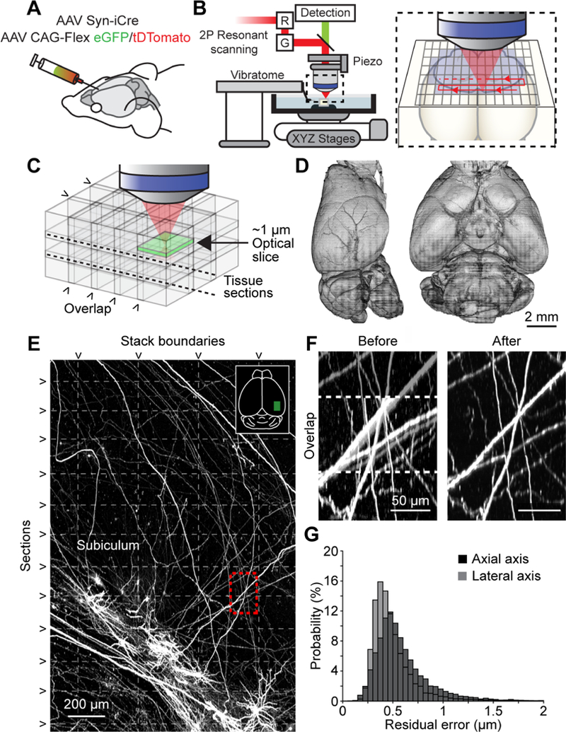
Imaging pipeline. (A) Animals were injected in targeted brain areas with a combination of a low-titer AAV Syn-iCre and a high-titer AAV CAG-Flex-(eGFP/tDTomato). (B) Two-photon microscope with an integrated vibratome. Inset, sequential imaging of partially overlapping image stacks. (C) Image stacks overlapped in x, y, and z. (D) Rendered brain volume after stitching (sample 2016–10-31 in Table S2). (E) Horizontal maximum intensity projection through a 1300 × 2000 × 600 μm³ volume of the motor cortex containing labeled somata and neurites. Horizontal dashed lines mark physical tissue sections; vertical dashed line represents stack boundaries. Dashed box is region shown in F. (F) Example of boundary region between two adjacent image stacks before (left) and after stitching (right). Dashed line indicates overlap region. (G) Residual stitching error in the lateral and axial directions. See also Table S1, S2, Figure S1, and Movie S1.

To enhance the throughput of our pipeline, we increased the number of cells that could be reconstructed per imaged brain. First, by injecting up to five separate areas per brain, we labeled larger numbers of cells, while retaining sparse labeling in any one brain region (Movie S1, Table S1). The fluorescent reporter for each injection site was chosen to minimize the overlap of axons of the same color (e.g. eGFP label for thalamus and tdTomato for the thalamus-projection zones in cortex). Next, we employed a whole-mount immunohistochemical labeling method to amplify the fluorescent signal. This improved the signal-to-noise ratio, especially for neurons that appeared dim with native fluorescence, and thus allowed for a larger portion of labeled neurons to be reconstructed (Table S2). Finally, to ensure optimal image quality throughout the entire sample, we developed a web service that monitored the data acquisition of the microscope (Figure S1F–H). Taken together, these improvements resulted in a progressive increase in the number of neurons that could be reconstructed per imaged brain (> 100 neurons in recent samples; Table S2).

Semi-automated reconstruction of complete neurons

Manual interventions during reconstruction remain a significant bottleneck in generating neuronal reconstructions (Economo et al., 2016). Even with specialized custom reconstruction software applied to precisely stitched brain volumes, a complex cortical neuron previously took approximately 1–3 weeks to be reconstructed in its entirety (Economo et al., 2016). To accelerate reconstruction, we developed a semi-automated reconstruction pipeline consisting of several components. A key first step in the reconstruction workflow is automated segmentation. A classifier trained to identify neurites, including axonal and dendritic processes, was applied to the imaged stacks. The derived probability map was thresholded, skeletonized, and fitted with line segments (Figure 2A and 2B; up to 100K segments per brain). Because crossing points were sometimes misidentified as branch points by the automated segmentation, segments were “broken” at all branch points and close crossing points, to be reconnected later using manual linking. This approach provided more accurate reconstructions compared to full automation. Generated segments covered the majority of axonal length (93% of total length, based on 27 neurons), keeping manual tracing to a minimum.

Figure 2.

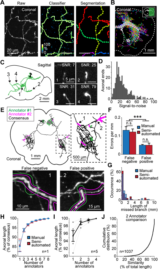
Complete semi-automated reconstruction of individual neurons. (A) Automated segmentation. Left, raw maximum intensity image of axons in the thalamus. Middle, probability map output from classifier. Right, segmentation result, with each detected segment depicted in a different color. (B) Coronal section through a sample with overlaid segmented neurites. (C) Left, sagittal view of a reconstructed cortical neuron. Arrows indicate location of axon endings shown on the right. Right, maximum projection of axon endings several millimeters away from the soma (1: 4.1 mm; 2: 4.9 mm; 3: 6.5 mm; 4: 4.6 mm). Numbers in top right show individual signal-to-noise ratios. (D) Distribution of image signal-to-noise ratio for axon endings (difference in intensity between the axon ending and surrounding background, divided by the standard deviation of background). (E) Establishing consensus in reconstructions produced by two annotators. Top, example reconstruction of a single neuron. Black, agreement between two annotators; green and magenta, unique segments detected by one of the two annotators. Inset, higher magnification view of dashed box on the left. Bottom, images of the areas of confusion numbered in the inset shown above. Colored outlines represent the reconstructions of the two annotators. (1) False-negative error, or a missed branch. (2) False-positive error consisting of an erroneously appended branch. (F) Frequency of each error-type for manual and semiautomated reconstructions. (G) Length distribution of missed neuronal branches for manual and semi-automated reconstructions. (H) Increase in accuracy as a function of the number of annotators reaching consensus. Accuracy is the proportion of axonal length that was correctly reconstructed. The consensus reconstruction from all eight annotators was defined as 100% accurate. (I) Same analysis as shown in H for 5 neurons across the brain with reconstructions from 4 annotators. (J) Cumulative distribution of reconstruction similarity between two annotators. Similarity is the proportion of axonal length present in the reconstructions of both annotators. Error bars ± SEM. ***: p < 0.001. See also Figure S2, S3, and Movie S2.

For manual linking and proofreading, we developed software for efficient three-dimensional visualization and annotation (Janelia Workstation; Murphy et al., 2014). The software allowed seamless exploration of the entire mouse brain at multiple resolutions with the overlaid auto-generated line segments. Human annotators used the Workstation to complete the reconstruction by proofreading the segmentation and linking appropriate segments (Movie S2; see STAR Methods). Multiple annotators worked collaboratively on the same brain volume concurrently. This semi-automated pipeline resulted in a more than five-fold increase in reconstruction speed compared to manual reconstruction, without loss in accuracy (manual: 4.5 ± 2.8 mm/hr; Economo et al., 2016; semi-automated: 25.2 ± 11.9 mm/hr). A typical cortical neuron with 10 centimeters of axon was completed in approximately 4 hours and a complex CA3 neuron of 27 centimeters in 8 hours.

Inaccurate reconstructions can arise from poor signal-to-noise ratio or other defects in the data. For this reason, we selectively reconstructed neurons with high and consistent fluorescent signal throughout the entire axonal arbor (Table S2). In these neurons, axonal endpoints were clearly identifiable even at locations far from the soma (Figure 2C, 2D and Figure S2), indicating that the entire arbor could be reliably reconstructed. Neurons that did not meet these criteria, for instance due to a gradual decrease in fluorescence along the axon, were not reconstructed.

Reconstruction errors can also arise from occasional attentional drift of individual annotators (Helmstaedter et al., 2011). For example, an annotator may overlook a branch point during proofreading and thus miss part of the axonal arbor. To measure these effects, multiple annotators (n = 8) independently traced the same cortical neuron (length: 11.5 cm; 274 branch points) and compared their reconstructions in pairs (Figure 2E). We considered the consensus reconstruction across all annotators as ground truth (100%). Reconstructions produced by a single annotator were typically accurate to 85.9 ± 9.1% of total axonal length, with a low rate of errors, mostly corresponding to missed branch points (1.8 ± 0.7 errors per cm; range 1.0 – 2.7; Figure 2F and 2G). Accuracy increased after two annotators produced a consensus reconstruction (93.7 ± 4.9% of total length). Adding a third annotator produced smaller gains in accuracy (96.5 ± 3.1% of total length; Figure 2H). The reconstructions were not degraded by the faster semi-automated reconstruction approach (Figure 2F–H). A similar analysis based on four annotators reconstructing four additional neurons produced comparable results (Figure 2I). To balance accuracy and throughput, every neuron in our database was reconstructed by two annotators. As expected, pairs of reconstructions were highly similar for the majority of neurons (87.7 ± 14.3% of total axonal length, n = 1037 neurons; Figure 2J). Based on the analysis presented above, the consensus of these paired reconstructions is expected to exceed 90% of the complete axonal arborization. This approach allowed us to accurately reconstruct the neuronal morphology of more than one thousand neurons.

Online database of more than 1,000 reconstructed neurons

Reconstructed neurons were registered to the Allen Mouse Common Coordinate Framework (CCF v3; Gilbert and Ng, 2018) using a landmark registration approach (Figure S3; see STAR Methods). More than 1,000 fully reconstructed and registered neurons were deposited in an online resource (www.mouselight.janelia.org; Movie S3). The web interface allows neurons to be searched based on Boolean logic using somatic and axonal target locations (Figures 3–6). Neuronal reconstructions can be viewed together with anatomical structures in 3D and also downloaded for offline analysis. Currently, the database contains projection neurons primarily from the thalamus (Figure 3, 7 and S4), hippocampus (Figure 4), cerebral cortex (Figures 5 and 6), and hypothalamus. Together their projections innervate 11% of the CCF v3 voxels (25 μm resolution), distributed across all major brain structures.

Figure 3.

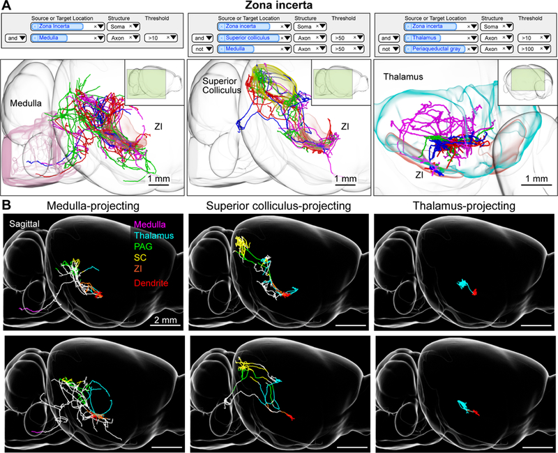
Zona incerta neurons. (A) Example queries (top) and 3d visualizations (bottom) for three projection groups in the zona incerta (ZI). Left, ZI neurons with axonal projections in the medulla. Middle, ZI neurons with projections in the superior colliculus but not the medulla. Right, ZI neurons with projections in the thalamus and not the periaqueductal gray. Inset shows perspective of shown area relative to the entire brain. (B) Examples of single ZI neurons belonging to the projection groups shown in A. Axons are color coded according to anatomical position (PAG: periaqueductal gray, SC: superior colliculus, ZI: zona incerta). Dendrites are shown in red. See also Figure S4 and movie S3.

Figure 6.

Thalamus-projecting neurons in the motor cortex. (A) Search query (top) and 3d visualization (bottom) for pyramidal tract (PT) neurons in the motor cortex with axons in the pons. (B) Sagittal view of single PT neurons that project to the thalamus (PT thalamus- projecting; green) or medulla (PT medulla-projecting; magenta) respectively. (C) PT neuron projections to different nuclei of the thalamus. Rows represent thalamic nuclei (PF: parafascicular nucleus, MD: mediodorsal nucleus, VM: ventral medial nucleus, PCN: paracentral nucleus, VAL: ventral anterior-lateral complex, PO: posterior complex). Columns correspond to individual neurons. The color of the heat map denotes the total number of axonal ends and branch points. The dashed white line separates neurons with dense innervation of the PF (PF-projecting) and those without (Other). (D) Left, sagittal view of PF-projecting neurons in shades of blue. Right, example image of axon in PF with varicosities. (E) Same area as in D, with PT thalamus-projecting neurons that do not project to PF in shades of red. (F) Search query (top) and 3d visualization (bottom) of layer 6 CT (L6-CT) neurons in the motor cortex. Neurons are identified by the presence of axons in the thalamus and the lack of projections to the pons. (G) Horizontal view of single L6-CT neurons and their axonal projections to the thalamus (green). Dendrites are red. (H) L6-CT neuron projections to thalamus. Rows, thalamic nuclei (PO: posterior complex, MD: mediodorsal nucleus, VM: ventral medial nucleus of the thalamus, VAL: ventral anterior-lateral complex of the thalamus, VPM: ventral posteromedial nucleus of the thalamus, PCN: paracentral nucleus, RT: reticular nucleus); columns represent individual neurons. The color of the heat map indicates the number of axon branches and ends. (I) Thalamic projections of example neurons (arrowheads in H). Left, dashed lines indicate the coronal views on the right. Greyscale images are from the Allen anatomical template. See also Figure S7 and Movie S4.

Figure 7.

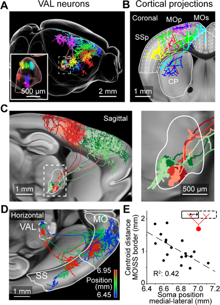
Cortical projections from neurons in the VAL complex of the thalamus. (A) Six VAL neurons and their axonal projections. (B) Coronal view of the same neurons. Dashed lines show position of cortical layers. (C) Left, sagittal view of two groups of VAL neurons with similar projection patterns in the posterior (red; n = 3 cells) or anterior (green; n = 3 cells) motor cortex. Right, higher magnification view of dashed box on the left. (D) Horizontal view of cortical projections of three neurons in caudomedial VAL, color coded according to their medial lateral position. White outline show locations of motor (MO) and sensory cortex (SS). (E) Relationship between somatic medial-lateral position and the average distance of the axonal centroid in the motor (MO) and sensory cortex (SS) to the border of those two areas (illustrated by inset). Positions are in CCF coordinates. Greyscale images are from the Allen anatomical template. See also Movie S5.

Figure 4.

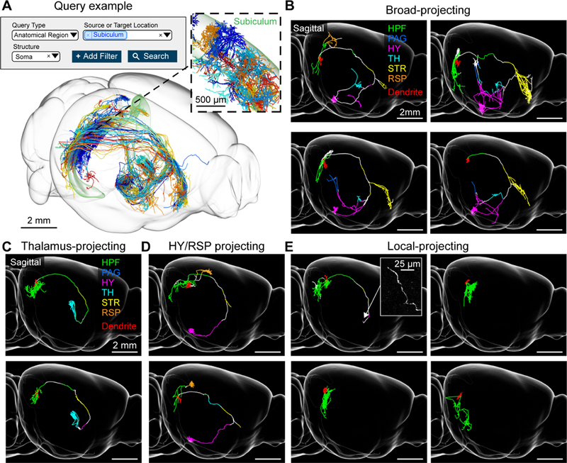
Subiculum neurons. (A) Example query requesting all neurons with somata in the subiculum (top) and the resulting 3d visualization (bottom). Inset, higher magnification view of area in dashed box showing the dendrites of the same cells (B) Examples of broad-projecting subiculum neurons with their axons color coded by anatomical position (HPF: hippocampal formation, PAG: periaqueductal gray, HY: hypothalamus, TH: thalamus, STR: striatum, RSP: retrosplenial cortex). Innervation in striatum is mostly confined to the lateral septum and nucleus accumbens. Dendrites are shown in red. (C) Thalamus-projecting neurons. (D) Hypothalamus/retrosplenial cortex projecting neurons. (E) Local-projecting neurons. Inset shows long-range axonal end of a local-projecting neuron that lacks varicosities. See also Figure S5.

Figure 5.

Motor cortex intratelencephalic neurons. (A) Search query (top) and 3d visualization (bottom) for intratelencephalic (IT) neurons in the motor cortex classified by lack of axons in thalamus or pons. Inset, higher magnification view of area in dashed box showing the dendrites of the same cells. (B) Innervation of telencephalic targets by IT neurons. Rows correspond to projection targets. Columns represent individual IT neurons. Color denotes the axonal length for that cell in a specific area. (C) Horizontal view of individual IT neurons with axons color coded according to their anatomical position. Dendrites are shown in red. See also Figure S6.

Our database allows discovery of novel projection classes. For example, the zona incerta (ZI) has been associated with diverse functions, including defensive behavior (Chou et al., 2018), appetite (Zhang and van den Pol, 2017) and sensory gating (Urbain and Deschênes, 2007). As a group, ZI neurons project to the medulla, midbrain, and thalamus (Oh et al., 2014; Sita et al., 2007), but little is known about the projections of individual neurons. A search for ZI neurons shows that neurons in rostral ZI fall into at least three projection classes. The groups project to the periaqueductal grey (PAG) and medulla (Figure 3; n = 4/12 cells), or PAG and superior colliculus (SC; n = 4/12), or thalamus (4/12 cells). Linking these projection subtypes to different behavioral states will require further investigation.

Dorsal subiculum contains at least four projection types

The dorsal subiculum, a major output structure of the hippocampus, has been extensively studied for its role in memory, navigation, and motivated behavior (Aggleton and Christiansen, 2015). Previous studies have identified a proximal-distal division (with respect to CA1) of pyramidal neurons in the dorsal subiculum that differ by gene-expression, electrophysiology, and connectivity (Cembrowski et al., 2018a). The database contains a large number of subiculum neurons (n = 73 cells; Figure 4A), allowing a detailed analysis (a previous analysis was based on 11 neurons; Cembrowski et al., 2018a).

Dorsal subiculum neurons fall into four projection groups (Figure 4B–E and S5). One group, consisting of neurons at relatively distal locations (Figure S5B and S5C), project to either the retrosplenial cortex (RSP, n = 4/27), hypothalamus (n = 6/27) or both of these areas (n = 17/27; Figure 4D). A second group, located at relatively proximal locations, project broadly to multiple targets, including the nucleus accumbens, lateral septal nucleus, thalamus, periaqueductal gray, and hypothalamus (n = 11; Figure 4B). The hypothalamic projections of these neurons were missed in previous bulk tracing studies (Cembrowski et al., 2018a), likely because neurons in proximal subiculum arborize in portions of the hypothalamus that were not targeted by those injections. A third group of subiculum neurons, positioned in between the distal and proximal groups, projects to the anterior dorsal thalamus (n = 21, Figure 4C). These three cell types overlap with the cell types described in previous studies (Cembrowski et al., 2018a, 2018b). A fourth group of subiculum neurons, widely distributed across the dorsal subiculum, consists of neurons with primarily local collaterals (n = 14), and in some cases one additional, unbranched long-range axon (n = 4; Figure 4E). Because neurons in the dorsal subiculum project to half a dozen areas in various combinations, previous studies using retrograde tracers in pairwise combinations failed to elucidate these complex projection patterns (Kim and Spruston, 2012; Naber and Witter, 1998).

Motor cortex: a diverse collection of projection types

Projection neurons in the cerebral cortex are known to have complex axonal arborizations (Binzegger et al., 2004; Economo et al., 2016, 2018; Han et al., 2018; Kita and Kita, 2012; Oberlaender et al., 2011; Shepherd, 2013). Our database contains motor cortex neurons corresponding to the major cortical projection classes: (1) intratelencephalic neurons (IT) in layers 2–6 (n = 189), (2) pyramidal tract neurons (PT) in layer 5b (n = 37), and (3) corticothalamic neurons (CT) in layer 6 (n = 73; Shepherd, 2013). Based on gene expression analysis, each class is thought to contain many cell types (Arlotta et al., 2005; Economo et al., 2018; Tasic et al., 2018).

IT neurons are some of the most diverse and morphologically complex cells in our database (Figure 5A and 5B). Analysis of 175 IT neurons in the database revealed projections that were mostly limited to the cortex and striatum, with more minor projections to the basolateral amygdala and the claustrum (Figure 5 and S6; Shepherd, 2013). Collectively, IT neurons projected to (from strongest to weakest projection) motor cortex, somatosensory cortex, insula, ectorhinal cortex, piriform cortex, visual cortex, claustrum, and basolateral amygdala. The majority of IT neurons crossed the corpus callosum to project bilaterally (n = 147/175). The axonal arbors of bilaterally projecting neurons were often strikingly mirror-symmetric across the midline (Yorke and Caviness, 1975), more so for L5 neurons than the others (p < 0.001, one-way ANOVA; L5: 0.36 ± 0.12 Jaccard similarity coefficient, L2/3: 0.26 ± 0.14, L6: 0.28 ± 0.09; calculated at 1 mm resolution, see STAR Methods). The majority of IT neurons also projected to the striatum (n = 148/175), either bilaterally (n = 97/175), ipsilaterally (n = 37/175), or contralaterally (n = 14/175).

Cortical projection neurons are often referred to by the efferent projection target of interest, typically identified by retrograde labeling or antidromic activation (e.g., ‘callosal projecting neurons’ or ‘corticostriatal neurons’; Fame et al., 2011; Shepherd, 2013; Turner and DeLong, 2000). In our data set, the vast majority of IT neurons project both to the striatum and across the corpus callosum. The proportion of axonal length in the striatum or cortex varied by more than one order of magnitude and was not dependent on the size of the axonal arbor (Figure S6A). In general, these neurons did not fall into discrete clusters and therefore defied traditional classifications, projecting instead to multiple targets in almost all possible combinations. For example, individual IT neurons can have up to 40 cm of axon and project to many distinct cortical areas and the striatum; other IT neurons project to a small subset of these areas (Figure 5C and S6B). This diversity in projection patterns is much greater than those observed in the subiculum or zona incerta and potentially forms a continuum.

Parallel projections from motor cortex to the thalamus

Our database contains numerous reconstructions from the motor cortex and thalamus (Figure 5–7 and S6–7), areas that are bidirectionally interconnected (Deschênes et al., 1994; Guo et al., 2017; Hunnicutt et al., 2014; Oh et al., 2014). Although the reciprocal connections between these areas have been studied, relatively little is known about the projections of individual cells.

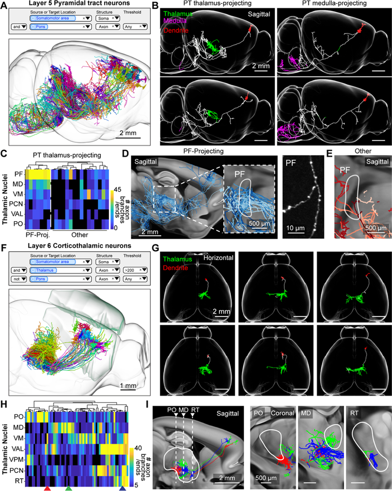
Cortical projections to the thalamus originate from layers 5 and 6 (Sherman, 2016). In layer 5 these projections arise from pyramidal tract (PT) neurons, which define layer 5b, and project to the midbrain, brainstem and spinal cord (Figure 6A). Their axons do not cross the corpus callosum to the contralateral hemisphere and have limited projections within cortex (Shepherd, 2013). Corticothalamic projections from layer 5 originate from a molecularly distinct subtype of PT neuron (PT thalamus-projecting) in the upper part of L5b (Figure 6B; Economo et al., 2018). These neurons innervate multiple areas of the thalamus, but lack arborizations in the medulla that are characteristic of PT neurons located in lower L5b (PT medulla-projecting; Movie S4).

Here we further subdivided the PT thalamus-projecting neurons (Figure 6C–E; Movie S4). One subgroup (n = 7/23 cells) had extensive axonal ramifications in the parafascicular (PF) and mediodorsal (MD) nucleus of the thalamus (Figure 6C). These cells also projected to common extra-thalamic targets: the external segment of the globus pallidus (GPe) and the nucleus of the posterior commissure (NPC; Figure S7A). Another subgroup projects to other parts of the thalamus, such as the ventral medial nucleus (VM), paracentral nucleus (PCN), and the posterior complex (PO) and did not project to GPe or NPC (Figure 6C–E and Figure S7B). These findings show that thalamus-projecting PT cells in the motor cortex fall into projection subtypes that have distinct targets (Movie S4). Additional studies are required to determine how these subtypes of thalamus-projecting PT neurons correspond to differences in gene expression and function.

We next investigated the organization of corticothalamic axons originating from layer 6 of the motor cortex (L6-CT). L6-CT cells project almost exclusively to the thalamus, apart from local collaterals in the cortex, and do not cross the corpus callosum (Figure 6F; n = 63 cells; Thomson, 2010). Compared to layer 5 PT thalamus-projecting neurons, individual L6-CT projections extended over a larger thalamic area (Figure 6G; L6-CT : area = 1.2 ± 0.4 mm³, p < 0.001, length = 40.8 ± 12.5 mm, p < 0.001; PT thalamus-projecting: area = 0.7 ± 0.4 mm³, length = 16.9 ± 10.7 mm; calculated at 200 μm resolution; see STAR Methods) and branched more within the thalamus (L6-CT = 80.3 ± 49.9 branch points, PT thalamus-projecting = 34.9 ± 26.7 branch points; p < 0.001).

Previous studies have subdivided L6-CT neurons in somatosensory cortex into two groups based on their projections to first-order (e.g. ventral posteromedial nucleus, VPM) or higher-order thalamus (e.g. PO; Hoerder-Suabedissen et al., 2018; Shima et al., 2016; Thomson, 2010); only first-order projecting neurons were found to project onto inhibitory neurons in the reticular nucleus (RT). In our data set, the L6-CT neurons in motor cortex are considerably more diverse than these previous studies suggested. We often observed dense projections in both first-order (VAL, VPM) and higher-order (PO, MD, VM) nuclei, either with or without arborizations in RT (Figure 6H and 6I). Additional studies will be required to determine whether L6-CT neurons in the motor cortex form discrete projection subtypes, or are part of a continuum of projection patterns.

L6-CT neurons in the somatosensory cortex project to sensory thalamus in a topographically organized manner (Deschênes et al., 1998). Our single-neuron reconstructions reveal a similar topographic organization in the motor cortex. L6-CT neurons in the posterior motor cortex sent their axonal projections to lateral regions of the thalamus (Figure S7C; R² = 0.31, p < 0.001 linear regression). Furthermore, these posterior neurons mostly remained on the ipsilateral side of the thalamus, unlike more anterior neurons that often crossed the midline (Figure S7C; R² = 0.17, p < 0.001 linear regression). Topographic maps organized along distinct axes were also seen within targeted thalamic nuclei of L6-CT neurons (Figure S7D–F).

VAL thalamus contains fine-scale projection maps

Neurons in the ventral anterior-lateral complex of the thalamus (VAL) project to a large area of the ipsilateral motor cortex (Bosch-Bouju et al., 2013), with additional projections to the somatosensory cortex (n = 34 cells). Some neurons also arborized in RT (n = 4/34) and/or the dorsal striatum (n = 14/34; Figure 7A and 7B; Kuramoto et al., 2009). Individual VAL neurons had arborizations within confined areas of the cerebral cortex. These projections were not random because groups of neighboring neurons in VAL had similar thalamocortical projections (Figure 7C). For example, neurons within the caudomedial VAL had two main axonal tufts located in the anterior motor and sensory cortex respectively (n = 18/34 cells; Figure 7D). These two branches were positioned around a common plane of symmetry that corresponded to the border between the motor and somatosensory cortical areas. The relative distance of each tuft to this anatomical border correlated with the neurons mediolateral position in VAL (R² = 0.42, p < 0.01 linear regression; Figure 7E; Movie S5). These findings show fine-scale topography between subregions of VAL and cortical areas of different modalities. Studying the axonal arbors of individual neurons therefore reveals organization of projections that are obscured with traditional bulk labeling approaches.

Discussion

We describe an imaging and reconstruction platform capable of producing complete neuronal reconstructions at unprecedented speed and scale. More than 1,000 fully reconstructed neurons are available in our online database (www.mouselight.janelia.org). Reconstruction of axonal arbors is a valuable step towards generating cellular circuit diagrams and classifying neurons based on morphology. Although our pipeline does not explicitly detect synapses, axonal arborizations contain an approximately constant density of synapses and axonal length is therefore a convenient surrogate for interareal connectivity (Braitenberg and Schüz, 1991; Shepherd et al., 2002). Our database represents a unique resource for the investigation of interareal connectivity and discovery of cell types based on axonal projections. Clustering based on these data identified new projection subtypes (Figure 3–6) and topographic gradients of single cell projections (Figure 7 and S7).

Previous large-scale studies of long-range projections have relied on bulk labeling to trace projections across brain areas (Hintiryan et al., 2016; Hooks et al., 2018; Hunnicutt et al., 2014; Oh et al., 2014; Zingg et al., 2014). These approaches effectively average across cell types with distinct projections, thus obscuring the detailed organization of individual axonal arbors.

Neurons with distinct projection patterns have traditionally been identified based on combinatorial retrograde labeling with multiple markers (Betley et al., 2013; Kim and Spruston, 2012; Naber and Witter, 1998; Pan et al., 2010). This approach is cumbersome because the number of required injections scales non-linearly with the number of projection targets. In addition, the spatial specificity is limited by the confinement of the injected tracer, and biases are produced by variable efficiency of tracer uptake in different brain regions and by different cell types; tracer uptake by axons of passage may also complicate these experiments. These limitations lead to potential errors in the detection of combinatorial projections. In contrast, complete neuronal reconstructions provide axonal projection maps at the finest levels of detail and unambiguously reveals the diversity of multi-areal projection patterns.

We relied on a viral labeling strategy using a low-titer AAV Syn-iCre and a high-titer fluorescent reporter to obtain a rich sampling of projection neurons (Table S1 and S2). However, this and other labeling techniques have biases in the transduction efficiency for different cell types. Our pipeline allows for diverse labeling methods, which counteracts these biases (Table S2; Chan et al., 2017; Harris et al., 2014; Xu et al., 2012). Reconstructions can be aggregated across brains and labeling methods to produce a more comprehensive atlas of neuronal morphologies.

Great progress has been made on methods for single-cell RNA sequencing (scRNA-seq), which now provides detailed transcriptomes of individual cells. Large-scale scRNA-seq measurements in the neocortex and other structures have identified known cell types and in addition also discovered additional transcriptomic clusters, which might correspond to newly discovered cell types (Cembrowski et al., 2018b; Shekhar et al., 2016; Tasic et al., 2016, 2018; Zeisel et al., 2018). Establishing the relationship between transcriptomic cluster and cell type requires validation with other types of information, typically neuronal structure. For example, the correspondence between transcriptomic clusters and retinal bipolar cells with distinct morphology is excellent (Shekhar et al., 2016). Distinct transcriptomic clusters of pyramidal tract neurons in the motor cortex correspond to different pyramidal tract neurons with axonal arborizations in either the medulla or thalamus (Economo et al., 2018). Recordings from these cell types revealed distinct activity that correlated either with the planning or execution of goal- directed movements. These studies illustrate how the structural cell types in our database can be linked to molecular cell types and neural function.

In the future, more efficient methods for linking molecular and morphological information will be critical for characterizing neuronal cell types. Since our histological treatments and imaging are non-destructive (i.e. they result in a series of preserved brain slices) our pipeline is amenable to post-hoc gene expression analysis by in-situ hybridization techniques and other types of molecular characterization (Chen et al., 2015; Eng et al., 2017; Shah et al., 2018). The synergy between large-scale genetic (Tasic et al., 2016; Zeisel et al., 2018) and morphological studies is primed to transform our understanding of how the brain is organized.

Single-neuron reconstructions have been performed in the past (Igarashi et al., 2012; Kita and Kita, 2012; Kuramoto et al., 2009; Lin et al., 2018; Wittner et al., 2007; Wu et al., 2014), but at low rates and often not to completion. For example, a single CA3 pyramidal neurons in the hippocampus (Wittner et al., 2007) was reconstructed over four months of manual tracing; a similar CA3 neuron in the MouseLight database was reconstructed within eight hours (Database identifier: AA0420, length = 27.3 cm). Several advances contributed to the throughput and accuracy required to produce our data set, including improved tissue processing, high-contrast imaging, automated segmentation, and 3d volumetric visualization for proofreading.

The precisely assembled image volume generated by our pipeline is amenable to even faster reconstructions using more advanced computational approaches. Much progress has been made towards fully automated tracing, but accuracy is still limiting (Acciai et al., 2016; Peng et al., 2015). In our pipeline, we segmented neurites in an automated manner, but the segments were linked into trees by manual proofreading. Combining automated segmentation with manual reconstruction allowed us to reconstruct complete neurons, including all termination zones, revealing the full complexity of axonal arbors. A complete characterization of the cell types of the mouse brain will likely require reconstructions of 100,000 neurons or more (assuming 1000 brain regions, an average of 10 cell types per brain region, and 10 measurements per cell type; Svoboda, 2011) over hundreds of brains using diverse labeling techniques. How can the required increase in throughput be achieved? Despite the advances presented here the speed of reconstructions is still limiting. One brain containing 100 neurons can be imaged in one week per microscope, and the imaging can be accelerated and parallelized. In contrast, with our current semi-automated workflow, reconstructing 100 neurons requires approximately 400 person-hours (10 person-weeks) of manual proofreading. Currently, all decision points (i.e. linking of automatically segmented neurites to a tree) are curated manually, which is the limiting step in reconstructions. We believe that a 10 to 100-fold acceleration in reconstruction speed is required and may be feasible if all but the most difficult decisions are performed by computer algorithms in a fully automated manner, for example using convolutional neural networks. Our database of gold-standard reconstructions will serve as training data for the machine learning algorithms that will be required to achieve these gains. Together with increased speeds in imaging, this enhanced reconstruction speed would make the goal of a full characterization of the cell types in the mouse brain achievable.

STAR Methods

Contact for reagent and resource sharing

Further information and requests for resources and reagents should be directed to and will be fulfilled by the Lead Contact, Jayaram Chandrashekar (chandrashekarj@janelia.hhmi.org).

Experimental model and subject details

Animals

Wild-type C57BL/6 animals were obtained from Charles River Laboratories. Rorb-IRES2-Cre (IMSR_JAX: 023526; Harris et al., 2014) and Sim1-Cre (IMSR_JAX: 006451; Balthasar et al., 2005) transgenic animals were obtained from The Jackson Laboratory. Adult females (> 8 weeks) were used for all experiments and were group housed with sex-matched littermates. Mice were healthy, had access to ad libitum food and water, and were housed in an enriched environment. No animals used in this study were used in previous procedures. All experimental protocols were conducted according to the National Institutes of Health guidelines for animal research and were approved by the Institutional Animal Care and Use Committee at Howard Hughes Medical Institute, Janelia Research Campus (Protocol #14–115).

Method details

Viral labeling

To achieve sparse labeling, we injected adult C57/BL6 mice with a combination of highly diluted adeno associated virus expressing Cre-recombinase (AAV Syn-iCre) and high-titer reporter virus coding for a fluorescent reporter (AAV CAG-Flex eGFP/tDTomato; Figure 1A). Multiple non-overlapping brain areas were labeled in each brain (Table S1 and Movie S1). For the Rorb-IRES2-Cre transgenic animal (2017–08-10, Table S2), sparsity was achieved using diluted Cre-dependent FLP-recombinase (AAV Syn-Flex-Flpo) and a FLP-dependent reporter virus (AAV CAG-FRT-eGFP/tDTomato;). The Sim1-Cre animal (2018–08-01, Table S2) received a systemic injection via the retro-orbital sinus with a mixture of Cre-dependent FLP-recombinase (PHP-eB-Syn-Flex-Flpo) and a FLP-dependent reporter virus (PHP-eB-CAG-FRT-3xGFP; Chan et al., 2017). High titer (> 10¹² GC/ml) viruses were obtained from the Janelia Research Campus Molecular Biology Core and diluted in sterile water when necessary.

Tissue preparation and clearing

Transfected mice were anesthetized with an overdose of isoflurane and then transcardially perfused with a solution of PBS containing 20 U/ml heparin (H3393, Sigma-Aldrich, St. Louis, MO) followed by a 4% paraformaldehyde solution in PBS. Brains were extracted and post-fixed in 4% paraformaldehyde at 4°C overnight (12–14 hours) and washed in PBS to remove all traces of excess fixative (PBS changes at 1 h, 6h, 12h, and 1 day).

For imaging of endogenous fluorescence, brains were delipidated by immersion in CUBIC-1 reagent for 3–7 days (Economo et al., 2016; Susaki et al., 2015). For amplification by immuno- labeling, brains were delipidated with a modified Adipo-Clear protocol (Chi et al., 2018). Brains were washed with methanol gradient series (20%, 40%, 60%, 80%, Fisher #A412SK) in Bin buffer (H₂O/0.1% Triton X-100/0.3 M glycine, pH 7; 4 mL/ brain; one hour / step). Brains were then immersed in 100% methanol for 1 hour, 100% dichloromethane (Sigma #270997) for 1.5 hours, and three times in 100% methanol for 1 hour. Samples were then treated with a reverse methanol gradient series (80%, 60%, 40%, 20%) in Bin buffer for 30 minutes each. All procedures were performed on ice. Samples were washed in Bin buffer for one hour and left overnight at room temperature; and then again washed in PTxwH buffer (PBS/0.1% Triton X-100/0.05% Tween 20/2 μg/ml heparin) with fresh solution after one and two hours and then left overnight.

After delipidation, selected samples were incubated in primary antibody dilutions in PTxwH for 14 days on a shaker (1:1000, anti-GFP, Abeam, #ab290; 1:600, anti-tDTomato, Sicgen, #ab8181). Samples were sequentially washed in 25ml PTxwH for 1, 2, 4, 8, and three times for 24 hours. Samples were incubated in secondary antibody dilutions in PTxwH for 14 days (Alexa Fluor 488 conjugated donkey-anti-rabbit IgG, 1:400, Invitrogen, #A21206; Alexa Fluor 546 conjugated donkey-anti-goat IgG, 1:400, Invitrogen, #A11056) and washed in PTxwH similar to descriptions above.

Brains were embedded in 12% (w/v) gelatin and fixed in 4% paraformaldehyde for 12 hours. Index matching for optical clarity was achieved by immersing the samples in solutions of 40% DMSO in 10 mM PB with increasing concentrations of D-Sorbitol (up to 40/60 w/v; see Economo et al., 2016) or in a solution of 40% OptiPrep (D1556, Sigma-Aldrich) in DMSO. The final imaging medium had a refractive index of 1.468 which allowed for imaging up to depths of 250 μm in the tissue without significant loss of fluorescence (Economo et al., 2016).

Microscope

Processed samples were imaged using a resonant scanner two-photon microscope imaging at million voxels per second (Figure 1B; Economo et al., 2016). The microscope is integrated with a motorized stage (XY: M-511.DD, Z: M-501-DG, Controller: C843; Physike Instrumente, Karlsruhe, Germany) and vibratome (Leica 1200S, Leica Microsystems, Wetzlar, Germany). Imaging was performed using a 40x/1.3 NA oil-immersion objective (#440752, Carl Zeiss, Oberkochen, Germany) attached to a piezo collar (P-725K.103 and E-665.CR, Physik Instrumente). Image stacks (385 × 450 × 250 μm³) were collected with a voxel size of 0.3 × 0.3 × 1 μm³ in two channels (red and green). The surface of the sample was automatically detected using the difference in autofluorescence between the tissue and the embedding gelatin. Scanning of the exposed brain block-face was then achieved by dividing it into smaller image stacks (Figure 1C). Overlap between adjacent stacks (25 μm) allowed feature-based registration and stitching (Figure S1A–E). After the block-face was imaged to a depth of 250 μm the vibratome removed 175 μm of tissue, leaving approximately 75 μm of overlap across imaged sections. The mouse brain was imaged in approximately one week. Signal quality was constant over this time.

To ensure robust and fault-proof processing of our large datasets, we created a custom software pipeline that facilitates the multi-step data processing in real time as the images are being acquired (Figure S1F–H; https://github.com/MouseLightProject/Mousel_ight-Acquisition-Pipeline). Success or failure of the processing of each tile for each task was tracked, logged, and reported in a graphical user interface (Figure S1H). Each imaged stack was analyzed for possible faults in imaging (e.g. air bubble in front of the objective) or sectioning (e.g. larger than expected slice thickness). In case of a detected fault the microscope was automatically shut down to allow for manual adjustments.

Feature-based volume stitching

A fully imaged brain consists of ~20k imaged stacks that need to be stitched to create a coherent volume. Accurate stitching is necessary to eliminate discontinuous neurites at the borders, which is critical for reliable reconstruction and automation. Standard methods involving linear transformations between adjacent tiles, following by global optimization, do not produce micrometer level precision (Bria and lannello, 2012; Chalfoun et al., 2017; Emmenlauer et al., 2009; Tsai et al., 2011). To account for non-linear deformations (caused by physical sectioning, optical field curvature etc.), we extended the descriptor based stitching framework we described previously (Economo et al., 2016) to all three dimensions (Figure S1A–E). First, blob-like objects were detected in individual tiles using a difference of Gaussian filter. These descriptors were matched between adjacent tiles in both x, y, and z directions using a coherent point drift algorithm (Myronenko and Song, 2010). Matched descriptors were then used to estimate a non- rigid transformation which mapped voxel locations to a target coordinate space while preserving the spatial ordering. For computational efficiency the transformation was represented as a set of barycentric transforms of 5×5×4 equally distributed control points in each stack (x, y, and z respectively).

3D visualization and reconstruction

For viewing and annotating terabyte-scale image stacks, each dataset (input tiles) was resampled into a common coordinate space according to the transforms determined during the stitching procedure. This produced a set of non-overlapping image stacks (output tiles) that spanned the imaged volume. Resampling was achieved by back-projecting each voxel in each output tile to the nearest sampled voxel. In regions where two or more input tiles overlapped, the maximum intensity was used for the corresponding location in the output tile. The resampling task was implemented on a cluster (64 nodes each with 32 cores and 512 GB RAM) of Intel CPUs with Advanced Vector Instructions 2 (AVX2) and parallel access to high- bandwidth network storage. The input tiles were partitioned into contiguous sets and traversed in Morton order to facilitate merging overlaps in memory. Execution was dominated by the time required to read and write data to disk. Data were resampled to 0.25 × 0.25 × 1 μm voxels, and stored on disk along with downsampled octree representations of the same volume for visualization at different spatial scales.

The imaged data was viewed and annotated in the Janelia Workstation (JW; https://github.com/MouseLightProject/workstation; Murphy et al., 2014; Movie S2). The JW allows low lag, multi-scale visualization of terabyte-scale image volumes, rendering of sub-volumes in three dimensions, and ergonomic annotation tools for tracing and proofreading. A detailed description of the JW will be published elsewhere.

Semi-automated segmentation

We trained a binary random forest classifier to identify axonal processes using five different appearance and shape features (Gaussian, Laplacian, gradient magnitude, difference of Gaussian, structure tensor Eigenvalues, Hessian of Gaussian Eigenvalues) at multiple spatial scales (σ = 0.3, 1, 1.6, 3.5, and 5 μm; llastik, Sommer et al., 2011). Training sets were created by pixel-based classification of axonal processes in regions containing different morphological features (axons close to the soma, termination zones etc.). The output of the classifier consisted of a probability stack where the value of each pixel reflects the likelihood of it belonging to an axon. A morphological skeleton (Lee et al., 1994) was then created by extracting the centerline of the classifier output after thresholding (> 0.5). For efficiency during visualization, we downsampled the resulting line segments to approximately 20 μm spacing in between nodes.

All segmented neurites were split into linear segments by separating them at their axonal branch points (Figure 2A and 2B; Movie S2). Several filtering steps were applied on the resulting segmentation to remove incorrectly identified processes. For instance, we used a path- length based pruning strategy where spurious branches (<15 μm) were deleted. Furthermore, a separate classifier was trained to identify auto-fluorescence originating from fine-scale vasculature and non-specific antibody binding. This approach generated up to 100,000 axonal segments per brain (length after split: 96.5 ± 155.4 μm, before: 263.4 ± 625.6 μm). The coverage of axonal processes by these generated segments was determined using fine-scale reconstructions (internode interval <5 μm) of all axonal projections in the caudoputamen of one sample and manually assigning fragments to each neuron (without merging).

Human annotators started from the soma and reconstructed neurons by linking neurite segments (Movie S2). Annotators in addition filled in parts of the neuron that may have been missed by the segmentation. The location of branch points and axonal endpoints were annotated to ensure that the entire axonal tree was reconstructed. Axons of neurons with insufficient expression became progressively dimmer and were eventually indistinguishable from the background fluorescence. These neurons were abandoned (median: 19% of cells in samples with more than 50 cells). Experienced annotators could identify these neurons after approximately 30 minutes of tracing. Two annotators independently reconstructed each neuron and compared their work to generate a consensus reconstruction (Figure 2E). Axons were distinguished from dendrites by their thickness, branching patterns, lack of dendritic spines, and overall length (Braitenberg and Schüz, 1991).

Sample registration

Imaged brains were aligned to the Allen Mouse Common Coordinate Framework (CCF) by taking a downsampled version of the entire sample volume (~5 × 5 × 15 μm voxel size) and registering it to the averaged Allen anatomical template (10 × 10 ×10 μm voxel size; Figure S3A and S3B) using the 3D Slicer software platform (slicer.org, Kikinis et al., 2014). First, parts of the brain that were not present in the anatomical template (e.g. the anterior olfactory bulb and posterior cerebellum/spinal cord), as well as the imaged gelatin, were cropped out of the sample volume. An initial automated intensity-based affine registration was then performed to align the sample to the anatomical template (BRAINSFit module, Johnson et al., 2007). An iterative landmark-registration processes, using thin-plate splines approximation, was then used to achieve a more precise registration to the template (LandmarkRegistration module, 110 ± 60 μm variation between independent registrations of the same sample). All registration steps were combined to generate a single displacement vector field which was used to align reconstructed neurons to the CCF. To determine the accuracy of the registration we measured the offset after registration between manually annotated anatomical boundaries and the Allen CCF. We found that the observed registration error was typically below 100 μm (Figure S3G).

Quantification and statistical analysis

All statistical analysis was performed in Matlab using custom made scripts. Unless stated otherwise, center and dispersion of bar plots represent mean ± SEM and descriptive statistics in the main text represent mean ± std. Significance was defined as p < 0.05, with the specific statistical test provided in main text or within associated figure legend. Sample sizes (n) can refer to the number of samples, brains, or cells and is clarified in the associated text. Significance conventions are as follows: NS: p ≥ 0.05; *: p < 0.05; **: p < 0.01; ***: p < 0.001 associated sample sizes are provided in the main text or within the figure legend. All reported position information is in Allen CCF coordinates.

Axonal length within an anatomical area was measured by taking all nodes within the given area and summing the distances to their parent nodes. Neuron order for all shown area heatmaps were determined using an average linkage hierarchical clustering algorithm based on Spearman correlation distance measures (except for Figure 5B and 6H which used Euclidean and Pearson correlation distances respectively). To minimize the influence of ‘axons-of-passage’ within the thalamus the number of axonal branch points and ends were used for clustering corticothalamic neurons. The weighted centroid of axonal projections was calculated by linearly resampling the axonal tree graph at 1 μm interval between connected nodes. Nodes within the area of interest were then selected using 3D meshes from the Allen CCF and their positions were averaged to derive the centroid. To exclude en passant axons, only neurons with at least three axonal ends in the area of interest were considered. Axonal area size was calculated by dividing the brain area of interest into isotropic voxels (200 × 200 × 200 μm³) and counting the number of voxels that an axon passed through. Bilateral symmetry of IT projections in the cortex was measured by similarly dividing the brain into isotropic voxels (at a coarser level of 1 × 1 × 1 mm³) and mirroring one hemisphere onto the other. Each voxel was scored for axon traversal on the ipsilateral and contralateral side. Symmetry was then calculated using the Jaccard similarity coefficient dividing the number of voxels that were positive for both hemispheres with the total number of positive voxels.

Data and software availability

All reconstructed neurons are available for download from the MouseLight NeuronBrowser (http://ml-neuronbrowser.janelia.org/). Matlab code for the performed analysis is available online (https://github.com/MouseLightProject/Analysis-Paper).

Supplementary Material

Figure S1.

Two-photon serial tomography imaging. Related to Figure 1. (A) Schematic representation of 3D volume stitching. Individual stacks are registered based on matching features with neighboring stacks in three dimensions. (B) Coronal maximum projection of one example imaged stack with two neighboring stacks shown in red. Dashed lines indicate the stack boundaries that mark the overlap region between two stacks. Inset shows higher magnification view of the overlap region with automatically detected image features marked as cyan crosses. (C) Example of the estimated error between neighboring tiles due to optical field curvature. (D) Left, neighboring image stacks along the optical axis. Right, stitching result. (E) Example of the estimated movement after sectioning in all three dimensions (see STAR Methods). (F) Sequential imaging of overlapping image stacks. Red line indicates the direction of imaging. (G) Schematic of online processing pipeline. Imaged stacks are automatically processed as they become available. Acquisition is halted if a fault is detected in the imaging. (H) Screenshot of acquisition pipeline software. Colored tiles indicate imaged stacks in different stages of processing.

Figure S2.

All axonal endings of one motor cortex neuron. Related to Figure 2. Top-left, 3d visualization of a intratelencephalic neuron in the motor cortex (AA0739 in the database). Caudoputamen (CP) is shown in blue. Small panels show maximum intensity projections of all axonal ends belonging to this neuron in the optimal viewing plane.

Figure S3.

Registration of reconstructed neurons to the Allen CCF. Related to Figure 2. (A) Coronal view of an imaged sample (left) and the corresponding section in the Allen anatomical template (right). (B) Estimated deformation in three dimensions of the same sample shown in A produced by the registration process. (C) Left, coronal section of the same sample after registration. Outline of Allen anatomical template shown in white. Right, higher magnification view of area marked on left with an overlay of the boundary for the thalamus (red) and hippocampus (green). (D) Visualizing sample data together with reconstructions in the NeuronBrowser. Example subiculum neuron seen here with a coronal plane from the corresponding sample and anatomical models of the periaqueductal gray (PAG) and medial mammillary nucleus (MM). Accuracy of registration can be judged in the browser by visual inspection. (E) Left, horizontal view of the thalamocortical projections from the ventral posteromedial nucleus (VPM) to the somatosensory cortex. Right, coronal view of the same neurons at the location of the dashed line on the left. White solid outline shows the location of the somatosensory cortex and the dashed line indicate the different cortical layers. Inset shows magnified view of VPM axons that project to layer 4 and the layer 5/6 boundary in accordance with previous findings (Lu and Lin, 1993; Petreanu et al., 2009). (F) Specificity of intratelencephalic (IT) neuronal projections to the basolateral amygdala (BLA). Left, horizontal view of IT neurons with projections to the BLA (shown in green). Inset shows magnified view of the area depicted with the dashed box on the left. White outline shows the boundary of the BLA.Right, sagittal view of the same neurons. (G) Spatial offset after registration between manually annotated anatomical boundaries and the Allen CCF. Left, high magnification coronal view of the anterodorsal nucleus, fasciculus retroflexus, and the subthalamic nucleus. The red, blue and green outlines show the location of the annotated regions in three different samples. The black outline shows the same area in the Allen CCF. Right, quantification of the spatial offset between the annotated areas and the Allen CCF. Spatial offset is the average difference between the weighted centroid of both areas along the rostral-caudal axis. Colored dots indicated the measured offset for each sample. Error bars ± SEM.

Figure S4.

Projections from neurons across thalamic nuclei. Related to Figure 3. (A) Search queries (top) and 3d visualization (bottom) for neurons with somata in different parts of the thalamus: ventromedial nucleus, ventral anterior-lateral complex, ventral posteromedial nucleus, and anteroventral nucleus. (B) Example of single thalamic neurons in the same areas shown in A. Axons are color coded according to their anatomical position (RSP: retrosplenial cortex, HPF: hippocampal formation). Neuron identifier (in database) shown in bottom-left.

Figure S5.

Projection groups in the subiculum. Related to Figure 4. (A) Clustering of dorsal subiculum neurons based on projection patterns. Left, manual grouping. Rows represent anatomical areas (NA: nucleus accumbens, PFC: prefrontal cortex, LEC: lateral entorhinal cortex, RSP: retrosplenial cortex, MEC: medial entorhinal cortex, VMH: ventromedial hypothalamic nucleus, Septum: lateral septal nucleus, NDB: diagonal band nucleus, PAG: periaqueductal grey, Ecto: ectorhinal cortex, SUB_{pre,para,post}: pre/para/post-subiculum, TH: thalamus, HY: hypothalamus). Columns correspond to individual neurons. Color denotes the axonal length in area. Bottom row color indicates the manually assigned group identity (red: broad, green: thalamus, blue: local, magenta: hypothalamus/restrosplenial cortex). Right, same data organized by hierarchical clustering. (B) Example horizontal image of the hippocampal formation from the Allen anatomical template. Dashed red line represents the proximal-distal axis in the subiculum in relation to CA1. (C) Somatic position on the proximal-distal axis by projection type. Gray circles represent individual cells. Error bars ± SEM. *: p < 0.05, **: p < 0.01, ***: p < 0.001 (D) Sagittal view of broad, thalamus, hypothalamus/retrosplenial cortex, or local-projecting subiculum neurons. Axons are color coded by anatomical position (HPF: hippocampal formation, PAG: periaqueductal grey, HY: hypothalamus, TH: thalamus, STR: striatum, RSP: retrosplenial cortex). Innervation in striatum is mostly confined to the lateral septum and nucleus accumbens. Neuron identifier (in database) shown in top-right.

Figure S6.

Projection patterns of intratelencephalic (IT) neurons in the motor cortex. Related to Figure 5. (A) Relationship between IT neuron fractional axonal length in the cortex and striatum (as proportion of total length). Dotted line indicates combined length of 100%. Neurons fall below this line due to axonal arbors in fiber tracts and other brain areas. (B) Horizontal view of IT neurons by cortical layer. Axons are color coded according to their localization. Neuron identifier (in database) shown in top-left.

Figure S7.

Thalamic innervation by neurons in the motor cortex. Related to Figure 6. (A) Left, sagittal view of PT thalamus-projecting neurons with arborizations in the parafascicular nucleus (PF-projecting neurons; red hues) and those without (Other; blue hues). Outlined area denotes the globus pallidus, external segment (GPe). Right, coronal view of same neurons in the nucleus of the posterior commisure (NPC). (B) Axonal length in GPe and NPC for projections types shown in A. Error bars ± SEM. ***: p < 0.001, two-sample t-test. (C) Left, horizontal view of L6-CT neurons in the motor cortex, color coded by anterior-posterior position. Center, relationship between somatic anterior-posterior position and medial-lateral position in the thalamus. Right, relationship between somatic position and axonal length in the contralateral thalamus. (D) Left, coronal view of L6-CT neurons with projections in RT, color coded by anterior-posterior position. Inset, higher magnification view of dashed box on the left. Center, example of varicosities on an axon within RT. Right, relationship between anterior-posterior position of the soma and axonal position in RT along the superior-inferior axis. (E) Same representation as in D showing relationship between somatic medial-lateral position and superior-inferior axonal position in PO. (F) Same representation as in D showing the relationship between somatic medial-lateral position and axonal anterior-posterior position in VAL. Dashed lines depict linear fit. Axonal position is measured as the weighted centroid of arbors within a region. Positions are in Allen CCF coordinates. Greyscale images are from the Allen anatomical template.

Movie S1.

Viral injection locations. Related to Figure 1. The movie shows the location of viral injections in the motor cortex, thalamus, hypothalamus and subiculum within a single imaged brain.

Movie S2.

Whole-brain visualization and semi-automated morphological reconstruction. Related to Figure 2. The movie shows the capability of the Janelia Workstation to traverse the entire mouse brain at multiple scales without lag. Time-lapse shows the semi-automated reconstruction workflow. Annotator links segments belonging to the same IT neuron to reconstruct a 30 mm axonal arbor in the cortex.

Movie S3.

MouseLight NeuronBrowser. Related to Figure 3. Movie illustrates the visualization and search capabilities of the MouseLight NeuronBrowser (mouselight.janelia.org).

Movie S4.

Projection subtypes of motor cortex pyramidal tract neurons. Related to Figure 6. Example of six pyramidal tract neurons that project to the medulla (magenta) or thalamus (green). Thalamus projecting pyramidal tract neurons each project to different parts of the thalamus: the posterior complex, ventral medial nucleus and parafascicular nucleus. Parafascicular-projecting neurons had unique projections to the external segment of the globus pallidus.

Movie S5.

Topographic organization of projections from the ventral anterior-lateral complex of the thalamus. Related to Figure 7. This movie shows how neurons in the caudomedial VAL project symmetrically to the motor and sensory cortex. Neurons that are located more laterally have arbors that are closer to the border of these two cortical areas. These arbors move closer together with more medial neurons.

Tables

Table S1. List of viral injection coordinates. Related to Figure 1.

Table S2. List of imaged brains. Related to Figure 1.

Highlights.

Efficient pipeline for brain-wide imaging and reconstruction of individual neurons

Searchable database containing more than 1,000 fully reconstructed neurons

In some brain areas projection neurons fall into discrete classes

Other projection neurons form a continuum of projection types

References

- Acciai L, Soda P, and lannello G (2016). Automated Neuron Tracing Methods: An Updated Account. Neuroinformatics 14, 353–367. [DOI] [PubMed] [Google Scholar]
- Aggleton JP, and Christiansen K (2015). The subiculum. In Progress in Brain Research, (Elsevier), 65–82. [DOI] [PubMed] [Google Scholar]
- Anderson JC, Binzegger T, Douglas RJ, and Martin KA (2002). Chance or design? Some specific considerations concerning synaptic boutons in cat visual cortex. J Neurocytol 31, 211–229. [DOI] [PubMed] [Google Scholar]
- Arlotta P, Molyneaux BJ, Chen J, Inoue J, Kominami R, and Macklis JD (2005). Neuronal Subtype-Specific Genes that Control Corticospinal Motor Neuron Development In Vivo. Neuron 45, 207–221. [DOI] [PubMed] [Google Scholar]
- Ascoli GA, and Wheeler DW (2016). In search of a periodic table of the neurons: Axonaldendritic circuitry as the organizing principle. BioEssays News Rev. Mol. Cell. Dev. Biol. 38, 969–976. [DOI] [PMC free article] [PubMed] [Google Scholar]
- Balthasar N, Dalgaard LT, Lee CE, Yu J, Funahashi H, Williams T, Ferreira M, Tang V, McGovern RA, Kenny CD, et al. (2005). Divergence of Melanocortin Pathways in the Control of Food Intake and Energy Expenditure. Cell 123, 493–505. [DOI] [PubMed] [Google Scholar]
- Betley JN, Cao ZFH, Ritola KD, and Sternson SM (2013). Parallel, Redundant Circuit Organization for Homeostatic Control of Feeding Behavior. Cell 155, 1337–1350. [DOI] [PMC free article] [PubMed] [Google Scholar]
- Binzegger T, Douglas RJ, and Martin KA (2004). A quantitative map of the circuit of cat primary visual cortex. J Neurosci 24, 8441–8453. [DOI] [PMC free article] [PubMed] [Google Scholar]
- Blasdel GG, and Lund JS (1983). Termination of afferent axons in macaque striate cortex. J. Neurosci. 3, 1389–1413. [DOI] [PMC free article] [PubMed] [Google Scholar]
- Bosch-Bouju C, Hyland BI, and Parr-Brownlie LC (2013). Motor thalamus integration of cortical, cerebellar and basal ganglia information: implications for normal and parkinsonian conditions. Front. Comput. Neurosci. 7, 163. [DOI] [PMC free article] [PubMed] [Google Scholar]
- Braitenberg V, and Schüz A (1991). Anatomy of the cortex: statistics and geometry (Berlin; New York: Springer-Verlag: ). [Google Scholar]
- Bria A, and lannello G (2012). TeraStitcher - A tool for fast automatic 3D-stitching of teravoxel-sized microscopy images. BMC Bioinformatics 13, 316. [DOI] [PMC free article] [PubMed] [Google Scholar]
- Cembrowski MS, Phillips MG, DiLisio SF, Shields BC, Winnubst J, Chandrashekar J, Bas E, and Spruston N (2018a). Dissociable Structural and Functional Hippocampal Outputs via Distinct Subiculum Cell Classes. Cell 173, 1280–1292. [DOI] [PubMed] [Google Scholar]
- Cembrowski MS, Wang L, Lemire AL, Copeland M, DiLisio SF, Clements J, and Spruston N (2018b). The subiculum is a patchwork of discrete subregions. ELife 7, e37701. [DOI] [PMC free article] [PubMed] [Google Scholar]
- Chalfoun J, Majurski M, Blattner T, Bhadriraju K, Keyrouz W, Bajcsy P, and Brady M (2017). MIST: Accurate and Scalable Microscopy Image Stitching Tool with Stage Modeling and Error Minimization. Sci. Rep. 7, 4988. [DOI] [PMC free article] [PubMed] [Google Scholar]
- Chan KY, Jang MJ, Yoo BB, Greenbaum A, Ravi N, Wu W-L, Sanchez-Guardado L, Lois C, Mazmanian SK, Deverman BE, et al. (2017). Engineered AAVs for efficient noninvasive gene delivery to the central and peripheral nervous systems. Nat. Neurosci. 20, 1172–1179. [DOI] [PMC free article] [PubMed] [Google Scholar]
- Chen KH, Boettiger AN, Moffitt JR, Wang S, and Zhuang X (2015). Spatially resolved, highly multiplexed RNA profiling in single cells. Science 348, aaa6090. [DOI] [PMC free article] [PubMed] [Google Scholar]
- Chi J, Wu Z, Choi CHJ, Nguyen L, Tegegne S, Ackerman SE, Crane A, Marchildon F, Tessier-Lavigne M, and Cohen P (2018). Three-Dimensional Adipose Tissue Imaging Reveals Regional Variation in Beige Fat Biogenesis and PRDM16-Dependent Sympathetic Neurite Density. Cell Metab. 27, 226–236. [DOI] [PubMed] [Google Scholar]
- Chou X, Wang X, Zhang Z, Shen L, Zingg B, Huang J, Zhong W, Mesik L, Zhang LI, and Tao HW (2018). Inhibitory gain modulation of defense behaviors by zona incerta. Nat. Commun. 9, 1151. [DOI] [PMC free article] [PubMed] [Google Scholar]
- Cowan RL, and Wilson CJ (1994). Spontaneous firing patterns and axonal projections of single corticostriatal neurons in the rat medial agranular cortex. J. Neurophysiol. 71, 17–32. [DOI] [PubMed] [Google Scholar]
- De Paola V, Holtmaat A, Knott G, Song S, Wilbrecht L, Caroni P, and Svoboda K (2006). Cell type-specific structural plasticity of axonal branches and boutons in the adult neocortex. Neuron 49, 861–875. [DOI] [PubMed] [Google Scholar]
- Deschênes M, Bourassa J, and Pinault D (1994). Corticothalamic projections from layer V cells in rat are collaterals of long-range corticofugal axons. Brain Res. 664, 215–219. [DOI] [PubMed] [Google Scholar]
- Deschênes M, Veinante P, and Zhang Z-W (1998). The organization of corticothalamic projections: reciprocity versus parity. Brain Res. Rev. 28, 286–308. [DOI] [PubMed] [Google Scholar]
- Economo MN, Clack NG, Lavis LD, Gerfen CR, Svoboda K, Myers EW, and Chandrashekar J (2016). A platform for brain-wide imaging and reconstruction of individual neurons. ELife 5, e10566. [DOI] [PMC free article] [PubMed] [Google Scholar]
- Economo MN, Viswanathan S, Tasic B, Bas E, Winnubst J, Menon V, Graybuck LT, Nguyen TN, Smith KA, Yao Z, et al. (2018). Distinct descending motor cortex pathways and their roles in movement. Nature 563, 79. [DOI] [PubMed] [Google Scholar]
- Emmenlauer M, Ronneberger O, Ponti A, Schwarb P, Griffa A, Filippi A, Nitschke R, Driever W, and Burkhardt H (2009). XuvTools: free, fast and reliable stitching of large 3D datasets. J. Microsc. 233, 42–60. [DOI] [PubMed] [Google Scholar]
- Eng C-HL, Shah S, Thomassie J, and Cai L (2017). Profiling the transcriptome with RNA SPOTs. Nat. Methods 14, 1153–1155. [DOI] [PMC free article] [PubMed] [Google Scholar]
- Fame RM, MacDonald JL, and Macklis JD (2011). Development, specification, and diversity of callosal projection neurons. Trends Neurosci. 34, 41–50. [DOI] [PMC free article] [PubMed] [Google Scholar]
- Gerfen CR, and Sawchenko PE (1984). An anterograde neuroanatomical tracing method that shows the detailed morphology of neurons, their axons and terminals: immunohistochemical localization of an axonally transported plant lectin, Phaseolus vulgaris leucoagglutinin (PHA-L). Brain Res. 290, 219–238. [DOI] [PMC free article] [PubMed] [Google Scholar]
- Ghosh S, Larson SD, Hefzi H, Marnoy Z, Cutforth T, Dokka K, and Baldwin KK (2011). Sensory maps in the olfactory cortex defined by long-range viral tracing of single neurons. Nature 472, 217–220. [DOI] [PubMed] [Google Scholar]
- Gilbert TL, and Ng L (2018). Chapter 3 - The Allen Brain Atlas: Toward Understanding Brain Behavior and Function Through Data Acquisition, Visualization, Analysis, and Integration In Molecular-Genetic and Statistical Techniques for Behavioral and Neural Research, Gerlai RT, ed. (San Diego: Academic Press; ), 51–72. [Google Scholar]
- Gong H, Xu D, Yuan J, Li X, Guo C, Peng J, Li Y, Schwarz LA, Li A, Hu B, et al. (2016). High-throughput dual-colour precision imaging for brain-wide connectome with cytoarchitectonic landmarks at the cellular level. Nat. Commun. 7, 12142. [DOI] [PMC free article] [PubMed] [Google Scholar]
- Greicius MD, Supekar K, Menon V, and Dougherty RF (2009). Resting-state functional connectivity reflects structural connectivity in the default mode network. Cereb. Cortex N. Y. N 1991 19, 72–78. [DOI] [PMC free article] [PubMed] [Google Scholar]
- Guo ZV, Inagaki HK, Daie K, Druckmann S, Gerfen CR, and Svoboda K (2017). Maintenance of persistent activity in a frontal thalamocortical loop. Nature 545, 181–186. [DOI] [PMC free article] [PubMed] [Google Scholar]
- Han Y, Kebschull JM, Campbell RAA, Cowan D, Imhof F, Zador AM, and Mrsic- Flogel TD (2018). The logic of single-cell projections from visual cortex. Nature 556, 51–56. [DOI] [PMC free article] [PubMed] [Google Scholar]
- Harris JA, Hirokawa KE, Sorensen SA, Gu H, Mills M, Ng LL, Bohn P, Mortrud M, Ouellette B, Kidney J, et al. (2014). Anatomical characterization of Cre driver mice for neural circuit mapping and manipulation. Front. Neural Circuits 8, 76. [DOI] [PMC free article] [PubMed] [Google Scholar]
- Helmstaedter M, Briggman KL, and Denk W (2011). High-accuracy neurite reconstruction for high-throughput neuroanatomy. Nat. Neurosci. 14, 1081–1088. [DOI] [PubMed] [Google Scholar]
- Hintiryan H, Foster NN, Bowman I, Bay M, Song MY, Gou L, Yamashita S, Bienkowski MS, Zingg B, Zhu M, et al. (2016). The mouse cortico-striatal projectome. Nat. Neurosci. 19, 1100–1114. [DOI] [PMC free article] [PubMed] [Google Scholar]
- Hoerder-Suabedissen A, Hayashi S, Upton L, Nolan Z, Casas-Torremocha D, Grant E, Viswanathan S, Kanold PO, Clasca F, Kim Y, et al. (2018). Subset of Cortical Layer 6b Neurons Selectively Innervates Higher Order Thalamic Nuclei in Mice. Cereb. Cortex 28, 1882–1897. [DOI] [PMC free article] [PubMed] [Google Scholar]
- Hooks BM, Papale AE, Paletzki RF, Feroze MW, Eastwood BS, Couey JJ, Winnubst J, Chandrashekar J, and Gerfen CR (2018). Topographic precision in sensory and motor corticostriatal projections varies across cell type and cortical area. Nat. Commun. 9, 3549. [DOI] [PMC free article] [PubMed] [Google Scholar]
- Hunnicutt BJ, Long BR, Kusefoglu D, Gertz KJ, Zhong H, and Mao T (2014). A comprehensive thalamocortical projection map at the mesoscopic level. Nat. Neurosci. 17, 1276–1285. [DOI] [PMC free article] [PubMed] [Google Scholar]
- Igarashi KM, Ieki N, An M, Yamaguchi Y, Nagayama S, Kobayakawa K, Kobayakawa R, Tanifuji M, Sakano H, Chen WR, et al. (2012). Parallel Mitral and Tufted Cell Pathways Route Distinct Odor Information to Different Targets in the Olfactory Cortex. J. Neurosci. 32, 7970–7985. [DOI] [PMC free article] [PubMed] [Google Scholar]
- Johnson H, Harris G, and Williams K (2007). BRAINSFit: Mutual Information Rigid Registrations of Whole-Brain 3D Images, Using the Insight Toolkit. 57, 11. [Google Scholar]
- Kawaguchi Y, Wilson C, and Emson P (1990). Projection subtypes of rat neostriatal matrix cells revealed by intracellular injection of biocytin. J. Neurosci. 10, 3421–3438. [DOI] [PMC free article] [PubMed] [Google Scholar]
- Kebschull JM, Garcia da Silva P, Reid AP, Peikon ID, Albeanu DF, and Zador AM (2016). High-Throughput Mapping of Single-Neuron Projections by Sequencing of Barcoded RNA. Neuron 91, 975–987. [DOI] [PMC free article] [PubMed] [Google Scholar]
- Kikinis R, Pieper SD, and Vosburgh KG (2014). 3D Slicer: A Platform for Subject-Specific Image Analysis, Visualization, and Clinical Support In Intraoperative Imaging and Image- Guided Therapy, Jolesz FA, ed. (New York, NY: Springer New York; ), 277–289. [Google Scholar]
- Kim Y, and Spruston N (2012). Target-specific output patterns are predicted by the distribution of regular-spiking and bursting pyramidal neurons in the subiculum. Hippocampus 22, 693–706. [DOI] [PMC free article] [PubMed] [Google Scholar]
- Kisvárday ZF, Kim D-S, Eysel UT, and Bonhoeffer T (1994). Relationship Between Lateral Inhibitory Connections and the Topography of the Orientation Map in Cat Visual Cortex. Eur. J. Neurosci. 6, 1619–1632. [DOI] [PubMed] [Google Scholar]
- Kita T, and Kita H (2012). The Subthalamic Nucleus Is One of Multiple Innervation Sites for Long-Range Corticofugal Axons: A Single-Axon Tracing Study in the Rat. J. Neurosci. 32, 5990–5999. [DOI] [PMC free article] [PubMed] [Google Scholar]
- Kuramoto E, Furuta T, Nakamura KC, Unzai T, Hioki H, and Kaneko T (2009). Two Types of Thalamocortical Projections from the Motor Thalamic Nuclei of the Rat: A Single Neuron-Tracing Study Using Viral Vectors. Cereb. Cortex 19, 2065–2077. [DOI] [PubMed] [Google Scholar]
- Kuramoto E, Ohno S, Furuta T, Unzai T, Tanaka YR, Hioki H, and Kaneko T (2013). Ventral Medial Nucleus Neurons Send Thalamocortical Afferents More Widely and More Preferentially to Layer 1 than Neurons of the Ventral Anterior-Ventral Lateral Nuclear Complex in the Rat. Cereb Cortex 1, 221–235. [DOI] [PubMed] [Google Scholar]
- Kuramoto E, Ohno S, Furuta T, Unzai T, Tanaka YR, Hioki H, and Kaneko T (2015). Ventral Medial Nucleus Neurons Send Thalamocortical Afferents More Widely and More Preferentially to Layer 1 than Neurons of the Ventral Anterior-Ventral Lateral Nuclear Complex in the Rat. Cereb. Cortex 25, 221–235. [DOI] [PubMed] [Google Scholar]
- Lee TC, Kashyap RL, and Chu CN (1994). Building Skeleton Models via 3-D Medial Surface Axis Thinning Algorithms. CVGIP Graph. Models Image Process. 56, 462–478. [Google Scholar]
- Lin H-M, Kuang J-X, Sun P, Li N, Lv X, and Zhang Y-H (2018). Reconstruction of Intratelencephalic Neurons in the Mouse Secondary Motor Cortex Reveals the Diverse Projection Patterns of Single Neurons. Front. Neuroanat. 12, 86. [DOI] [PMC free article] [PubMed] [Google Scholar]
- Lu SM, and Lin RC (1993). Thalamic afferents of the rat barrel cortex: a light- and electron- microscopic study using Phaseolus vulgaris leucoagglutinin as an anterograde tracer. Somatosens. Mot. Res. 10, 1–16. [DOI] [PubMed] [Google Scholar]
- Luppi P-H, Fort P, and Jouvet M (1990). lontophoretic application of unconjugated cholera toxin B subunit (CTb) combined with immunohistochemistry of neurochemical substances: a method for transmitter identification of retrogradely labeled neurons. Brain Res. 534, 209–224. [DOI] [PubMed] [Google Scholar]
- Markov NT, Ercsey-Ravasz MM, Ribeiro Gomes AR, Lamy C, Magrou L, Vezoli J, Misery P, Falchier A, Quilodran R, Gariel MA, et al. (2014). A Weighted and Directed Interareal Connectivity Matrix for Macaque Cerebral Cortex. Cereb. Cortex 24, 17–36. [DOI] [PMC free article] [PubMed] [Google Scholar]
- Murphy S, Rokicki K, Bruns C, Yu Y, Foster L, Trautman E, Olbris D, Wolff T, Nern A, Aso Y, et al. (2014). The janelia workstation for neuroscience. Keyst. Big Data Biol. San Franc. Ca. [Google Scholar]
- Myronenko A, and Song X (2010). Point Set Registration: Coherent Point Drift. IEEE Trans. Pattern Anal. Mach. Intell. 32, 2262–2275. [DOI] [PubMed] [Google Scholar]
- Naber PA, and Witter MP (1998). Subicular efferents are organized mostly as parallel projections: A double-labeling, retrograde-tracing study in the rat. J. Comp. Neurol. 393, 284–297. [PubMed] [Google Scholar]
- Oberlaender M, Boudewijns ZSRM, Kleele T, Mansvelder HD, Sakmann B, and de Kock CPJ (2011). Three-dimensional axon morphologies of individual layer 5 neurons indicate cell type-specific intracortical pathways for whisker motion and touch. Proc. Natl. Acad. Sci. 108, 4188–4193. [DOI] [PMC free article] [PubMed] [Google Scholar]
- Oh SW, Harris JA, Ng L, Winslow B, Cain N, Mihalas S, Wang Q, Lau C, Kuan L, Henry AM, et al. (2014). A mesoscale connectome of the mouse brain. Nature 508, 207–214. [DOI] [PMC free article] [PubMed] [Google Scholar]
- Ohno S, Kuramoto E, Furuta T, Hioki H, Tanaka YR, Fujiyama F, Sonomura T, Uemura M, Sugiyama K, and Kaneko T (2012). A Morphological Analysis of Thalamocortical Axon Fibers of Rat Posterior Thalamic Nuclei: A Single Neuron Tracing Study with Viral Vectors. Cereb. Cortex 22, 2840–2857. [DOI] [PubMed] [Google Scholar]
- Pan WX, Mao T, and Dudman JT (2010). Inputs to the Dorsal Striatum of the Mouse Reflect the Parallel Circuit Architecture of the Forebrain. Front. Neuroanat. 4, 147. [DOI] [PMC free article] [PubMed] [Google Scholar]
- Parent M, and Parent A (2006). Single-axon tracing study of corticostriatal projections arising from primary motor cortex in primates. J. Comp. Neurol. 496, 202–213. [DOI] [PubMed] [Google Scholar]
- Peng H, Hawrylycz M, Roskams J, Hill S, Spruston N, Meijering E, and Ascoli GA (2015). BigNeuron: Large-Scale 3D Neuron Reconstruction from Optical Microscopy Images. Neuron 87, 252–256. [DOI] [PMC free article] [PubMed] [Google Scholar]
- Petreanu L, Huber D, Sobczyk A, and Svoboda K (2007). Channelrhodopsin-2-assisted circuit mapping of long-range callosal projections. Nat. Neurosci. 10, 663–668. [DOI] [PubMed] [Google Scholar]
- Petreanu L, Mao T, Sternson SM, and Svoboda K (2009). The subcellular organization of neocortical excitatory connections. Nature 457, 1142–1145. [DOI] [PMC free article] [PubMed] [Google Scholar]
- Portera-Cailliau C, Weimer RM, Paola VD, Caroni P, and Svoboda K (2005). Diverse Modes of Axon Elaboration in the Developing Neocortex. PLoS Biol 3, e272. [DOI] [PMC free article] [PubMed] [Google Scholar]
- Ropireddy D, Scorcioni R, Lasher B, Buzsâki G, and Ascoli GA (2011). Axonal Morphometry of Hippocampal Pyramidal Neurons Semi-Automatically Reconstructed After InVivo Labeling in Different CA3 Locations. Brain Struct. Funct. 216, 1–15. [DOI] [PMC free article] [PubMed] [Google Scholar]
- Shah S, Takei Y, Zhou W, Lubeck E, Yun J, Eng C-HL, Koulena N, Cronin C, Karp C, Liaw EJ, et al. (2018). Dynamics and Spatial Genomics of the Nascent Transcriptome by Intron seqFISH. Cell 174, 363–376. [DOI] [PMC free article] [PubMed] [Google Scholar]
- Shekhar K, Lapan SW, Whitney IE, Tran NM, Macosko EZ, Kowalczyk M, Adiconis X, Levin JZ, Nemesh J, Goldman M, et al. (2016). Comprehensive Classification of Retinal Bipolar Neurons by Single-Cell Transcriptomics. Cell 166, 1308–1323. [DOI] [PMC free article] [PubMed] [Google Scholar]
- Shepherd GM (2013). Corticostriatal connectivity and its role in disease. Nat Rev Neurosci 14, 278–291. [DOI] [PMC free article] [PubMed] [Google Scholar]
- Shepherd GM, and Harris KM (1998). Three-dimensional structure and composition of CA3- -CA1 axons in rat hippocampal slices: implications for presynaptic connectivity and compartmentalization. J Neurosci 18, 8300–8310. [DOI] [PMC free article] [PubMed] [Google Scholar]
- Shepherd GMG, Raastad M, and Andersen P (2002). General and variable features of varicosity spacing along unmyelinated axons in the hippocampus and cerebellum. Proc. Natl. Acad. Sci. 99, 6340–6345. [DOI] [PMC free article] [PubMed] [Google Scholar]
- Sherman SM (2016). Thalamus plays a central role in ongoing cortical functioning. Nat. Neurosci. 19, 533–541. [DOI] [PubMed] [Google Scholar]
- Shima Y, Sugino K, Hempel CM, Shima M, Taneja P, Bullis JB, Mehta S, Lois C, and Nelson SB (2016). A Mammalian enhancer trap resource for discovering and manipulating neuronal cell types. ELife 5, e13503. [DOI] [PMC free article] [PubMed] [Google Scholar]
- Sita LV, Elias CF, and Bittencourt JC (2007). Connectivity pattern suggests that incerto-hypothalamic area belongs to the medial hypothalamic system. Neuroscience 148, 949–969. [DOI] [PubMed] [Google Scholar]
- Sommer C, Straehle C, Kothe U, and Hamprecht FA (2011). Ilastik: Interactive learning and segmentation toolkit. In 2011 IEEE International Symposium on Biomedical Imaging: From Nano to Macro, (Chicago, IL, USA: IEEE), 230–233. [Google Scholar]
- Susaki EA, Tainaka K, Perrin D, Yukinaga H, Kuno A, and Ueda HR (2015). Advanced CUBIC protocols for whole-brain and whole-body clearing and imaging. Nat. Protoc. 10, 1709–1727. [DOI] [PubMed] [Google Scholar]
- Svoboda K (2011). The past, present, and future of single neuron reconstruction. Neuroinformatics 9, 97–98. [DOI] [PubMed] [Google Scholar]
- Tasic B, Menon V, Nguyen TN, Kim TK, Jarsky T, Yao Z, Levi B, Gray LT, Sorensen SA, Dolbeare T, et al. (2016). Adult mouse cortical cell taxonomy revealed by single cell transcriptomics. Nat. Neurosci. 19, 335–346. [DOI] [PMC free article] [PubMed] [Google Scholar]
- Tasic B, Yao Z, Graybuck LT, Smith KA, Nguyen TN, Bertagnolli D, Goldy J, Garren E, Economo MN, Viswanathan S, et al. (2018). Shared and distinct transcriptomic cell types across neocortical areas. Nature 563, 72–78. [DOI] [PMC free article] [PubMed] [Google Scholar]
- Thomson AM (2010). Neocortical layer 6, a review. Front. Neuroanat. 4, 13. [DOI] [PMC free article] [PubMed] [Google Scholar]
- Tsai C-L, Lister JP, Bjornsson CS, Smith K, Shain W, Barnes CA, and Roysam B (2011). Robust, globally consistent and fully automatic multi-image registration and montage synthesis for 3-D multi-channel images. J. Microsc. 243, 154–171. [DOI] [PMC free article] [PubMed] [Google Scholar]
- Turner RS, and DeLong MR (2000). Corticostriatal Activity in Primary Motor Cortex of the Macaque. J. Neurosci. 20, 7096–7108. [DOI] [PMC free article] [PubMed] [Google Scholar]
- Urbain N, and Deschênes M (2007). Motor Cortex Gates Vibrissal Responses in a Thalamocortical Projection Pathway. Neuron 56, 714–725. [DOI] [PubMed] [Google Scholar]
- Veenman CL, Reiner A, and Honig MG (1992). Biotinylated dextran amine as an anterograde tracer for single- and double-labeling studies. J. Neurosci. Methods 41, 239–254. [DOI] [PubMed] [Google Scholar]
- Wittner L, Henze DA, Zâborszky L, and Buzsâki G (2007). Three-dimensional reconstruction of the axon arbor of a CA3 pyramidal cell recorded and filled in vivo. Brain Struct. Funct. 212, 75–83. [DOI] [PMC free article] [PubMed] [Google Scholar]
- Wu H, Williams J, and Nathans J (2014). Complete morphologies of basal forebrain cholinergic neurons in the mouse. ELife 3, e02444. [DOI] [PMC free article] [PubMed] [Google Scholar]
- Xu NL, Harnett MT, Williams SR, Huber D, O’Connor DH, Svoboda K, and Magee JC (2012). Nonlinear dendritic integration of sensory and motor input during an active sensing task. Nature 492, 247–251. [DOI] [PubMed] [Google Scholar]
- Yorke CH, and Caviness VS (1975). Interhemispheric neocortical connections of the corpus callosum in the normal mouse: A study based on anterograde and retrograde methods. J. Comp. Neurol. 164, 233–245. [DOI] [PubMed] [Google Scholar]
- Zeisel A, Hochgerner H, Lönnerberg P, Johnsson A, Memic F, van der Zwan J, Häring M, Braun E, Borm LE, La Manno G, et al. (2018). Molecular Architecture of the Mouse Nervous System. Cell 174, 999–1014. [DOI] [PMC free article] [PubMed] [Google Scholar]
- Zhang X, and van den Pol AN (2017). Rapid binge-like eating and body weight gain driven by zona incerta GABA neuron activation. Science 356, 853–859. [DOI] [PMC free article] [PubMed] [Google Scholar]
- Zingg B, Hintiryan H, Gou L, Song MY, Bay M, Bienkowski MS, Foster NN, Yamashita S, Bowman I, Toga AW, et al. (2014). Neural Networks of the Mouse Neocortex. Cell 156, 1096–1111. [DOI] [PMC free article] [PubMed] [Google Scholar]
Associated Data
This section collects any data citations, data availability statements, or supplementary materials included in this article.
Supplementary Materials