Building Atomic Models Based on Near Atomic Resolution cryoEM Maps with Existing Tools

Abstract

The EMDataBank Validation Challenge was a challenging task for students newly introduced to the cryoEM and molecular modeling fields. However, the competition provided an effective space for student modelers to discover and explore the potentials of atomic modeling and refinement by practicing on published atomic structures. Here, by employing manual molecular modeling programs such as Coot, Phenix, and Chimera, we have regularized and improved three targets. The T20S proteasome and TRPV1 ion channel allowed us to broaden our understanding of our techniques while the 70S ribosome served as a challenge to test the limits of our abilities. We were successful in our efforts to improve each of our models and provide here our cohesive methodology for de novo modeling with and without homology models, which may serve as a starting point for other undergraduates and researchers just entering the realm of cryoEM. Additionally, we provide some constructive criticism to facilitate the introduction of said undergraduates and researchers into cryoEM in the future.

Introduction

CryoEM has emerged as the tool of choice to obtain near-atomic resolution maps of complexes ranging in molecular weight from tens to thousands of kilodaltons. To maximize the value of such maps, it is necessary to derive atomic models so that molecular interactions within such complexes can be described and analyzed in chemical terms. To this end, atomic modeling based on density has benefited from many powerful graphical tools. Molecular modeling programs are great visualization platforms that allow for the prediction, assembly, and analysis of a wide variety of macromolecules. In the presence of growing modeling technology, protein structure prediction programs are also helpful tools to utilize during the modeling process. As the technology of cryoEM continues to improve, the resolution of cryoEM maps will undoubtedly reach atomic level. This enables automated model building from tools such as phenix.map_to_model (Terwilliger et al., 2018), ARP/wARP (Pereira and Lamzin, 2017), and Buccaneer (Cowtan, 2006), especially with partial models as an input. However, in this competition, we emphasize that manual modeling remains an essential step to the modeling process, at least while the resolution of high-resolution cryoEM maps remains in the near-atomic range. Even as map resolution continues to draw closer to atomic range, manual modeling may still be vital as a conceptual starting point to understand the advantages and drawbacks of various current and future automated model-building tools.

Atomic modeling is not only a process of reconstructing atomic structures, but also a great educational device for general biochemistry and molecular biology. Students new to cryoEM and molecular modeling can find it difficult to picture three-dimensional models without a visualization tool. Molecular modeling programs allow them to interact with the atomic structures to uncover side chain interactions, binding pockets, and catalytic regions; these same programs can ultimately allow students to begin building and refining their own atomic models. All of these tasks can be conducted through automated and manual modeling programs. Indeed, newcomers to the field of cryoEM often face the daunting task of deciding which of these tools to use in order to perform the most efficient practice.

Towards this end, a team of five undergraduate students was chosen to study atomic modeling tools and techniques via participation in the EMDataBank Modeling Challenge. During this challenge, our team chose to refine three target models, the T20S proteasome, TRPV1 ion channel, and E. coli 70S ribosome, each representing different types of protein function. During this competition, we successfully refined our target models primarily through manual model building based on near-atomic resolution cryoEM maps, ultimately arriving at a “best practice” to manual atomic modeling for cryoEM maps.

Methods

Initial Model Selection and Evaluations

For this competition, eight challenge targets were provided, each with a near-atomic resolution cryoEM map and a published atomic model. The TRPV1 ion channel (Liao et al., 2013), T20S proteasome (Li et al., 2013), and E. coli 70S ribosome (Li et al., 2015) were selected by our team based on their sizes, map resolutions, and level of modeling difficulty. The objective of our approach was to improve the modeling statistics of the initial structure by removing cis bonds, regularizing misfit residues, and identifying Ramachandran plot outliers. These selected models were evaluated manually using two atomic modeling programs, UCSF Chimera version 1.10 (Pettersen et al., 2004) and Coot version 0.8.2 (Emsley et al., 2010). The TRPV1 ion channel and T20S proteasome maps were not modified prior to model refinement; however, the E. coli 70S ribosome map was segmented in Chimera to facilitate our efforts. Using these programs, we identified regions in each complex for improvement.

Structure Refinement

Regions identified for improvement were subsequently subjected to structure refinement as follows. Before initiating refinement, each of the selected models was split, if necessary, into its subunits in UCSF Chimera due to large map size (70S ribosome) or the presence of high-order symmetry (T20S proteasome). Areas requiring minor refinements were corrected by the Coot tools ‘Real Space Refine Zone’, ‘Regularize Zone’, and ‘Rotate Translate’ in order to improve model-to-map fit and model statistics, e.g. decreasing the ‘outlier’ percentage of the Ramachandran plot. Specific outlier residues were selected and regularized until their conformation coordinates placed the residues in the ‘allowed regions’ of the Ramachandran plot. This process was repeated until the percentage of outliers in the plot could not be reduced further. Larger misfit residue ranges were remodeled from scratch with the ‘C-alpha Baton Mode’ and ‘Mainchain’ functions, which allowed us to manually build a poly-alanine backbone within the density. Alanine residues were then mutated to the correct amino acid sequence with ‘Mutate Residue Range’, and the regions were again refined with the aforementioned tools. Once each subunit had completed individual regularization, the whole atomic model was assembled through the symmetry command in Chimera, if necessary.

The real space refinement command in Phenix (Afonine et al., 2013) was applied to all models after manual refinement. Ramachandran plot outliers, allowed, and favored regions, rotamer outliers, EMRinger Score (Barad et al., 2015), and Molprobity (Chen et al., 2010) Clash Score were validation tools provided in addition to the refined model. Each target was manually inspected after Phenix refinement in order to guarantee proper model-map alignment.

All figures were prepared in UCSF Chimera.

Results and Discussion

The UCLA undergraduate team was composed of one first-year and four second-year students, majoring in Microbiology and Biochemistry. While tackling this modeling challenge, we applied our background knowledge from each field to analyze each target model. Members had varying degrees of experience in molecular modeling, with some being familiar with Coot and Chimera and others completely new to the modeling field. All of us utilized tutorials provided on the CCP4 website (Winn et al., 2011) and practiced on determined structures in order to understand the various functions and tools of the modeling programs.

Among the target models we chose, the proteasome and ion channel were much smaller atomic structures than the ribosome and consequently easier to work with. However, choosing large models such as the ribosome allowed us to test the limits and boundaries of the skills we learned throughout the competition.

Improved models

The quality of each atomic structure and its respective density map was visualized and analyzed through Coot and UCSF Chimera. We inspected for the presence of side chain compatibility and overall model fit to the density map. The proteasome, ion channel, and ribosome had 3.3 Å, 3.4 Å, and 3.6 Å resolution maps, respectively. For the most part, the quality of these maps was sufficient to allow us to identify not only carbon backbones, but also individual amino acid sidechains.

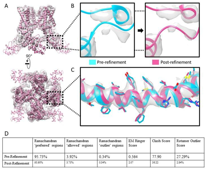
The TPRV1 ion channel is made up of 4 chains with C4 symmetry (Liao et al., 2013). In the central region, the model already had a good correlation to the map, owing to the higher local resolution in this region (Figure 1A). Many of the core alpha helices near the symmetry axis received only minor adjustments aimed at optimizing steric constraints and rotamer orientation (Figure 1C). Major refinements were made near the N-terminus of the chain, farther from the symmetry axis, where the resolution deteriorates. Many of the free loops in this region were not originally fit to the cryoEM density. In Coot, we used local real space refinement to remodel these loops to the strongest densities in the immediate area with attention to steric constraints and preservation of the overall tertiary structure (Figure 1B). The initial pre-refinement Ramachandran plot had 95.73% preferred, 3.92% allowed, and 0.34% outliers, and the initial model had an EMRinger Score of 0.564, Clash Score of 77.90, and Rotamer outliers of 27.79%. Our final refined model had a Ramachandran plot of 95.90% preferred, 3.75% allowed, and 0.34% outliers. From Phenix, we obtained the EMRinger Score of 2.07, Clash Score of 36.22, and Rotamer Outlier of 2.84% (Figure 1D).

Figure 1: TRPVI ion channel structure and side chain fit to density.

(A) Overview and goodness of fit, as well as, demonstration of higher central resolution vs lower outer resolution. (B) Major remodeling of free loops into strong, nearby densities. (C) Minor refinement in the higher resolution region. (D) Comparison of model statistics between the pre- and post-refined models.

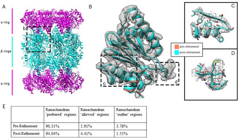
The T20S proteasome contains two beta-rings sandwiched between two alpha-rings (Li et al., 2013) (Figure 2A). During refinement, one alpha and beta subunit were regularized independently of each other and their copies before being recombined, and the full structure was regenerated by applying D7 symmetry in Chimera. The initial model fit well to its map and both alpha and beta subunits were completely modeled, making baton building unnecessary (Figure 2B). Longer sidechains were more likely to be bent outside of their electron density, which may have contributed to the poor fit of a four-residue loop in the beta subunit, framed by cis-bonded residues T21/M22 and N24/F25, that was noted by the authors of the original paper (Li et al., 2013). Manual refinement in Coot and Chimera corrected the poorly-modeled loops in the beta-ring such that the cis bonds were replaced with trans bonds (Figure 2C) and the misplaced alpha carbons were fully contained inside the density while these and Phenix improved the positions of other large sidechains relative to the map. Initially, the Ramachandran plot contained 90.31% preferred, 5.91% allowed, and 3.78% outlier residues. The post-refinement Ramachandran plot contained 94.04% preferred, 4.41% allowed, and 1.55% outlier residues (Figure 2E).

Figure 2: Side chain alignment improvements for beta ring in T20S proteasome.

(A) Overview with differing subunits colorized. (B) General changes made to one beta subunit, chain Z. (C) Residues 123–142 from the same chain, showing the model’s fit to the map as well as changes from the old model. (D) Residues 20–25 of the same chain, containing the cis-bonded residues T21/M22 and N24/F25. (E) Comparison of model statistics between the pre- and post-refined models.

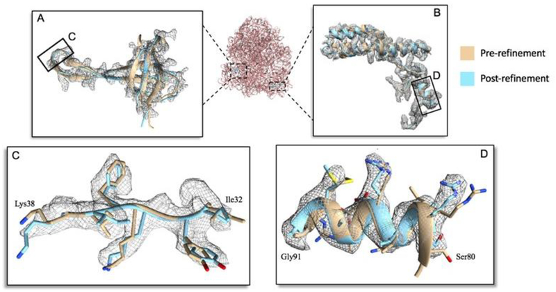
The 70S ribosome consists of the large ribosomal subunit (LSU) and the small ribosomal subunit (SSU) (Li et al., 2015). The model was regularized by its subunits using its corresponding 3.6Å map. The initial protein had a good model-to-map fitting, and the majority of the proteins of the LSU and SSU were completely modeled. The RNA model was also not extensively modified, as each nucleotide appeared in strong nucleic acid density throughout the map. All cis bonds were removed from the model except for the cis bond between Val96 and Pro97 on chain c of the SSU. Although the carbon backbones were well modeled within the map, many large sidechains were regularized and corrected for mismatched rotamer conformations (Figure 3C and 3D).

Figure 3: Side chain alignment improvement in 70S ribosome.

(A) Chain q and (B) chain n of the small ribosomal subunits comparison between pre-refined and post-refined model. (C) Residue ranges of 32–38 and (D) 80–91 show improved side chain to density fit.

The ribosome was deposited as 3ja1.cif.gz; from this we extracted a .cif file on which to begin our refinements in Coot and Chimera. However, the enormity of this complex was such that Chimera would promptly crash upon opening the .cif file. Additionally, Coot would only display some (but not all) of the chains inside the ribosome. Computational limitations (e.g., on personal laptops) may have contributed to these shortfalls. In order to begin refinement, we found it necessary to convert the .cif file into .pdb using the cif2pdb tool (Bernstein and Bernstein, 1996). However, that presented us with a new set of issues. The pdb file format can only support five-character atom numbers (maximum value 99,999) and single-character chain identifiers (maximum 62 chains, accounting for upper- and lowercase letters and 10 digits); however, the eukaryotic ribosome contains approximately 83 unique chains, with some deposited coordinate sets containing upwards of 400,000 atoms. We were able to exceed the 62-chain limit by using two-character chain IDs; Other workarounds are possible, but they cause a host of other issues (e.g., resetting numbering after reaching 99,999 atoms creates duplicate atom labels). Alternatively, newer file formats may be used, such as mmCIF or PDBx, explicitly created to handle large supramolecular complexes. These formats impose no limitations on atom count and allow for four-character chain IDs (Westbrook and Fitzgerald, 2009).

Lessons Learned and Best Practices

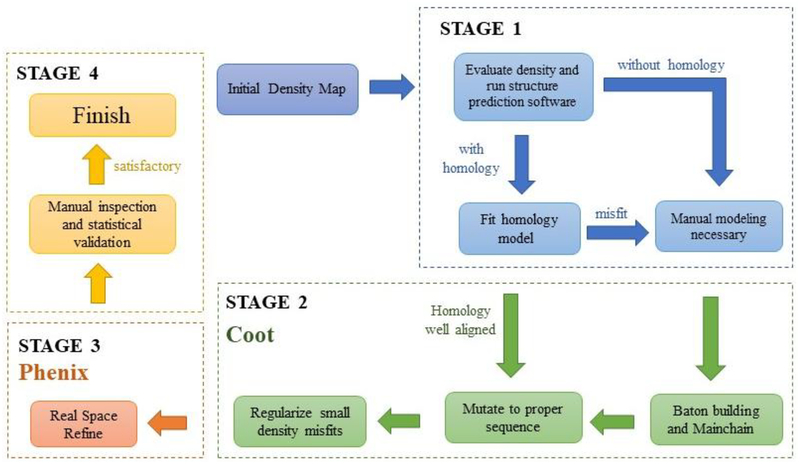
Refinement of published models was the main objective of the competition. The competition provided us with near-atomic resolution maps ranging from 3.3 Å to 3.6 Å as well as published benchmark models to improve and ultimately, compare to verify progress. De novo modeling was unnecessary. However, in realistic situations, atomic models are not always available. In order to solve an atomic structure, a de novo model may be necessary in the absence of homologous (conserved secondary structure) models. While an increasing number of programs that are capable of modeling high-resolution structures (Adams et al., 2010), many intermediate resolution structures still present challenges to such automated programs. Modeling in these conditions can be daunting for first-time modelers. To that end, we present our workflow for de novo modeling of cryoEM maps in the presence and absence of existing homology models (Figure 4). While de novo modeling from cryoEM density maps is not novel per se, a compilation of such a “best practice” into a single workflow based on our own experiences should facilitate newcomers to quickly become proficient modelers.

Figure 4: Best practice methodology for cryoEM atomic modeling.

Our methodology for building atomic models starting from new density maps in the presence and absence of homology models in four main stages. Stage 1: Initial inspection of density map De novoand assessment of homology model. Stage 2: modeling and analysis in Coot. Stage 3: Real Space Refinement in Phenix. Stage 4: Final inspection of the model.

Stage 1: Evaluation of density map and assessment of homology model

The initial map should be inspected for side chain densities in order to manually map some amino acid residues in a primary sequence to certain regions of the map. It is frequently ideal to begin prediction from large-sidechain (e.g., aromatic) densities rather than from perceived N- and C-terminal ends, as densities may be repeatedly broken by loop flexibility or for other reasons. Once the density has been evaluated, one should check for existing homology models. Although the homology model may not perfectly align to the density, it can provide essential information about the overall fold and even carbon backbone placement within the density. Structural prediction programs, such as Phyre2 (Kelley et al., 2015), and public databases, such as GenBank (Coordinators, 2016), can provide homologies by cross-referencing primary sequences with other sequences in their databases. However, if a homology model does not exist or fit the density, de novo modeling is necessary.

Stage 2: De novo modeling in Coot

Manual modeling can be handled in Coot. If the map is too large for certain Coot functions, it can be segmented in Chimera. Using the function ‘C-alpha Baton Mode’, a foundation of baton atoms will outline the coordinates of the α-carbons with respect to the density map. Afterwards, ‘Mainchain’ will create an alanine backbone from the baton atoms. Applying ‘Mutate Residue Range’ to the poly-alanine chain will convert the peptide into the proper amino acid sequence. Large sidechain markers such as phenylalanine, arginine, and tryptophan can help with sequence assignment. Once one or several regions have been registered to the sequence, the remainder of the protein should be buildable given that the backbone is traceable and not significantly broken. Residue ranges should be renumbered with ‘Renumber Residue’ in order to match the proper sequence number. Minor regularization changes can be conducted through ‘Real Space Refine Zone’, ‘Regularize Zone’, and ‘Rotate Translate’ tools. In difficult core regions of the protein where clashes become unavoidable, the ‘Sphere Refinement’ tool and MolProbity Interactive Dots are useful to improve geometry and fit without increasing clash score.

Stage 3: Real Space Refinement in Phenix

Once the structure has been built, real space refinement in Phenix should be conducted on the model. This operation will run automated regularizations as well as provide statistics for Ramachandran, Rotamer outliers, EMRinger score, and Molprobity clash score. In cases where the output model geometry is poor, feeding the manually built structure to phenix.geometry_minimization and using the result as the input for phenix.real_space_refine may yield improved geometry and fit. The exact parameters may differ based on protein and density quality, so it may take several tries to properly optimize Phenix. Reciprocal space refinement tools such as Refmac may also be used to refine the model (Skubák et al., 2004).

Stage 4: Inspection of the refined model

Manual refinement should be again implemented to adjust residues which may have been jostled out of the density map or into their neighbors during automated refinement. Changes here can include improvements to the Ramachandran plot, geometry, rotamers, and cis bond validations. Residues should be inspected to prevent overlapping sidechains. Molprobity should be used to check the model again after manual refinement to ensure that no extra clashes were introduced and that the geometry and fit have been maintained or improved. If the result is satisfactory, then the process is complete. If the result is unsatisfactory, repeating Stages 2 or 3 and adjusting the process will be necessary to obtain the optimized structure.

Conclusions

In summary, cryoEM is a challenging field for newcomers to enter, due in part to the difficulty in visualizing microscopic biomacromolecules and the wide variety of tools with which researchers can inspect and manipulate the molecular models. Five undergraduate researchers entered the EMDataBank Validation Challenge in order to thoroughly explore the molecular modeling programs Coot, UCSF Chimera, and Phenix while refining previously published benchmark molecules. The undergraduate team produced substantial refinements while also formulating a methodology which can be applied by any future cryoEM researchers, whether they are constructing models de novo or with homology models and other guides.

Overall, although our team was able to improve target coordinates, many gains were subtle, indicating that the original published models were generally of high quality. In some poorly resolved regions with limited resolution, such as that in TRPV1 (Fig. 1B), the published models exhausted the information provided by the map. As such, we were only able to make minor improvements, again suggesting that the original authors were thorough in their model building process.

References

- Adams PD, Afonine PV, Bunkoczi G, Chen VB, Davis IW, Echols N, Headd JJ, Hung LW, Kapral GJ, Grosse-Kunstleve RW, McCoy AJ, Moriarty NW, Oeffner R, Read RJ, Richardson DC, Richardson JS, Terwilliger TC, Zwart PH, 2010. PHENIX: a comprehensive Python-based system for macromolecular structure solution. Acta Crystallogr D Biol Crystallogr 66, 213–221. [DOI] [PMC free article] [PubMed] [Google Scholar]
- Afonine P, Headd J, Terwilliger T, Adams P, 2013. New tool: phenix. real_space_refine. Computational Crystallography Newsletter 4, 43–44. [Google Scholar]
- Barad BA, Echols N, Wang RY, Cheng Y, DiMaio F, Adams PD, Fraser JS, 2015. EMRinger: side chain-directed model and map validation for 3D cryo-electron microscopy. Nature methods 12, 943–946. [DOI] [PMC free article] [PubMed] [Google Scholar]
- Bernstein FC, Bernstein HJ, 1996. Translating mmCIF data into PDB entries. Acta Cryst. A 52. [Google Scholar]
- Chen VB, Arendall WB, Headd JJ, Keedy DA, Immormino RM, Kapral GJ, Murray LW, Richardson JS, Richardson DC, 2010. MolProbity: all-atom structure validation for macromolecular crystallography. Acta Crystallographica Section D: Biological Crystallography 66, 12–21. [DOI] [PMC free article] [PubMed] [Google Scholar]
- Coordinators NR, 2016. Database resources of the National Center for Biotechnology Information. Nucleic Acids Res 44, D7–19. [DOI] [PMC free article] [PubMed] [Google Scholar]
- Cowtan K, 2006. The Buccaneer software for automated model building. 1. Tracing protein chains. Acta Crystallographica Section D: Biological Crystallography 62, 1002–1011. [DOI] [PubMed] [Google Scholar]
- Emsley P, Lohkamp B, Scott WG, Cowtan K, 2010. Features and development of Coot. Acta Crystallogr D Biol Crystallogr 66, 486–501. [DOI] [PMC free article] [PubMed] [Google Scholar]
- Kelley LA, Mezulis S, Yates CM, Wass MN, Sternberg MJ, 2015. The Phyre2 web portal for protein modeling, prediction and analysis. Nat Protoc 10, 845–858. [DOI] [PMC free article] [PubMed] [Google Scholar]
- Li W, Liu Z, Koripella RK, Langlois R, Sanyal S, Frank J, 2015. Activation of GTP hydrolysis in mRNA-tRNA translocation by elongation factor G. Science advances 1. [DOI] [PMC free article] [PubMed] [Google Scholar]
- Li X, Mooney P, Zheng S, Booth CR, Braunfeld MB, Gubbens S, Agard DA, Cheng Y, 2013. Electron counting and beam-induced motion correction enable near-atomic-resolution single-particle cryo-EM. Nature methods 10, 584–590. [DOI] [PMC free article] [PubMed] [Google Scholar]
- Liao M, Cao E, Julius D, Cheng Y, 2013. Structure of the TRPV1 ion channel determined by electron cryo-microscopy. Nature 504, 107–112. [DOI] [PMC free article] [PubMed] [Google Scholar]
- Pereira J, Lamzin VS, 2017. A distance geometry-based description and validation of protein main-chain conformation. IUCrJ 4, 657–670. [DOI] [PMC free article] [PubMed] [Google Scholar]
- Pettersen EF, Goddard TD, Huang CC, Couch GS, Greenblatt DM, Meng EC, Ferrin TE, 2004. UCSF Chimera--a visualization system for exploratory research and analysis. Journal of computational chemistry 25, 1605–1612. [DOI] [PubMed] [Google Scholar]
- Skubák P, Murshudov GN, Pannu NS, 2004. Direct incorporation of experimental phase information in model refinement. Acta Crystallographica Section D: Biological Crystallography 60, 2196–2201. [DOI] [PubMed] [Google Scholar]
- Terwilliger TC, Adams PD, Afonine PV, Sobolev OV, 2018. A fully automatic method yielding initial models from high-resolution electron cryo-microscopy maps. bioRxiv, 267138. [DOI] [PMC free article] [PubMed] [Google Scholar]
- Westbrook JD, Fitzgerald PM, 2009. The PDB format, mmCIF formats, and other data formats. Structural Bioinformatics 44. [PubMed] [Google Scholar]
- Winn MD, Ballard CC, Cowtan KD, Dodson EJ, Emsley P, Evans PR, Keegan RM, Krissinel EB, Leslie AG, McCoy A, 2011. Overview of the CCP4 suite and current developments. Acta Crystallographica Section D 67, 235–242. [DOI] [PMC free article] [PubMed] [Google Scholar]