Processing of Natural Temporal Stimuli by Macaque Retinal Ganglion Cells

Abstract

This study quantifies the performance of primate retinal ganglion cells in response to natural stimuli. Stimuli were confined to the temporal and chromatic domains and were derived from two contrasting environments, one typically northern European and the other a flower show. The performance of the cells was evaluated by investigating variability of cell responses to repeated stimulus presentations and by comparing measured to model responses. Both analyses yielded a quantity called the coherence rate (in bits per second), which is related to the information rate. Magnocellular (MC) cells yielded coherence rates of up to 100 bits/sec, rates of parvocellular (PC) cells were much lower, and short wavelength (S)-cone-driven ganglion cells yielded intermediate rates. The modeling approach showed that for MC cells, coherence rates were generated almost exclusively by the luminance content of the stimulus. Coherence rates of PC cells were also dominated by achromatic content. This is a consequence of the stimulus structure; luminance varied much more in the natural environment than chromaticity. Only approximately one-sixth of the coherence rate of the PC cells derived from chromatic content, and it was dominated by frequencies below 10 Hz. S-cone-driven ganglion cells also yielded coherence rates dominated by low frequencies. Below 2–3 Hz, PC cell signals contained more power than those of MC cells. Response variation between individual ganglion cells of a particular class was analyzed by constructing generic cells, the properties of which may be relevant for performance higher in the visual system. The approach used here helps define retinal modules useful for studies of higher visual processing of natural stimuli.

There is growing interest in the way the visual system processes natural stimuli. Theoretical studies have used the statistical properties of stimuli from natural environments to predict spatial, temporal, and chromatic properties of various stages in visual processing (Srinivasan et al., 1982; Field, 1987; Atick, 1992; van Hateren, 1993; Dong and Atick, 1995; Olshausen and Field, 1997; van Hateren and Ruderman, 1998; for review, see Simoncelli and Olshausen, 2001). Natural, or at least naturalistic, stimuli have been used to physiologically investigate system function under normal environmental conditions. Species studied have ranged from invertebrates (Laughlin, 1981; van Hateren, 1992; Passaglia et al., 1997; Kern et al., 2001; Lewen et al., 2001; van Hateren and Snippe, 2001) through nonmammalian vertebrates (Vu et al., 1997; Berry, 2000) to mammals (Dan et al., 1996; Baddeley et al., 1997; Stanley et al., 1999; Vinje and Gallant, 2000). Study of primates is of particular interest in that they are the only mammals with trichromatic vision (Jacobs, 1993), and the visual capabilities of Old World primates are close to those of human. The macaque retina is a suitable locus for such a study, because ganglion cell types and their receptor and bipolar inputs are physiologically and anatomically well characterized (Kaplan et al., 1990; Dacey, 2000), and this can aid interpretation of responses to natural scenes.

Although our final goal is a full spatiotemporal and chromatic analysis of ganglion cell responses to natural stimuli, we begin with a simpler stimulus, a spatially homogenous field modulated only in time and spectral properties. The results are conceptually and computationally easier to analyze than those of full spatiotemporal stimuli, because the stimulus contains only two (time and spectrum) rather than four dimensions (when two spatial ones are added). Furthermore, many complex properties of the visual system, such as luminance and contrast gain controls, are already present in the time domain. We here attempt to capture responses to naturalistic stimuli in these dimensions, before attempting a full spatiotemporal model.

We used two different examples of a temporal stimulus, which we call chromatic time series of intensities (CTSIs). One was derived from a typical northern European environment, and the other was recorded from a flower show, which provided a different distribution of chromaticities (see Fig. 1). Stimuli were presented while responses were recorded from magnocellular (MC), parvocellular (PC), or short wavelength (S) cone-driven ganglion cells. We showed that linear models do not describe responses to natural stimuli well and developed nonlinear models that perform more satisfactorily. These models are developed for two main purposes. First, they allow us to analyze and quantify how information on luminance and spectral aspects of the stimuli are distributed among the different classes of ganglion cells. Second, they form a step toward the development of full spatiotemporal models that could be used as preprocessing modules for studies of higher visual processing.

Fig. 1.

Characteristics of the stimuli. A,x–y chromaticity coordinates of the stimulus recorded in the environment of the laboratory and played back on the LEDs of the Maxwellian view. B,x–y chromaticity coordinates of the flower show, as presented on the monitor. C, Normalized power spectra of the two stimuli. The power spectra were normalized by dividing by the square of the average illuminance of the stimuli, 1179 td for the LEDs (laboratory environment) and 222.2 td for the display (flower show). Frequencies are smoothed (averaged with a group of neighboring frequencies, with the group size proportional with frequency). D, E, Histograms of illuminance values of the stimulus from the laboratory environment and the flower show. F, Comparison of achromatic (a) and chromatic contrast (c_lm,c_s) in the flower show stimulus; see Materials and Methods for details.

MATERIALS AND METHODS

Preparation and recording. Ganglion cell activity was recorded from the retina of the anesthetized macaque (Macaca fascicularis). The animals were initially sedated with an intramuscular injection of ketamine (10 mg/kg). Anesthesia was maintained with inhaled isoflurane (0.2–2%) in a 70:30 N₂O/O₂ mixture. Local anesthetic was applied to points of surgical intervention. EEG and electrocardiogram were monitored continuously to ensure animal health and adequate depth of anesthesia. Muscle relaxation was maintained by a constant infusion of gallamine triethiodide (5 mg · kg⁻¹ · hr⁻¹, i.v.) with accompanying dextrose Ringer's solution (5 ml/hr). Body temperature was kept close to 37.5°. End tidal CO₂ was adjusted to close to 4% by adjusting the rate of respiration. All procedures were approved by the State of Lower Saxony Animal Welfare Committee and the Animal Care Committee of State University of New York College of Optometry.

A tungsten-in-glass recording microelectrode was introduced to the retina via a scleral hole using established techniques. The details of the preparation can be found in Lee et al. (1989). The location of the receptive field of each cell was mapped onto a tangent screen 114 cm from the eye. Cell identification was achieved using a battery of tests including chromatic sensitivity and time course of responses and other tests shown to reliably distinguish between MC and PC cells and those with S-cone input (Lee et al., 1989). Eccentricity of receptive fields ranged between 5 and 15°. The results presented in this article are based on 42 ganglion cells recorded from six animals. Partial measurements on another 35 cells from nine animals were fully consistent with those reported here.

Stimuli. Measurements on retinal ganglion cells were performed with two different naturalistic stimuli (“laboratory environment” and “flower show”) that were measured in two alternative environments, using different measurement equipment and different equipment to present the stimuli to the macaque retina.

The laboratory environment stimulus was recorded near the laboratory of one of the authors (Groningen, August). This environment consisted of many shades of green and brown (bushes, a variety of plants, grass, soil) but also contained flower beds and some manmade materials (pavement, concrete, buildings). The environment was scanned during walking with a hand-held optical device consisting of a lens focused onto a pinhole in front of a light guide. The resulting angular sensitivity of the detector had a full width at half-maximum of 8.7 arc min. The light was split (through a dichroic mirror, a half-silvered mirror, and spectral filters) into three chromatic channels, each equipped with a photomultiplier (Hamamatsu H5701-50). By combining filters (Edmund Optics), we tuned the three chromatic channels to approximately match the spectral sensitivities of the long (L), middle (M), and short wavelength (S) cones. A linear transformation of the three photomultiplier outputs was then used to improve the fidelity of the cone excitations.

During the sample period, signals from the photomultipliers were recorded on a portable DAT-recorder (Sony PC-208A). The resulting three signals were down-sampled and transformed to be presented on a Maxwellian view system with three light-emitting diodes (LEDs) with dominant wavelength 460, 554, and 638 nm (Lee et al., 1990). LED intensity was driven by a frequency-modulated pulse train that gave a highly linear output. Stimuli were presented at a sample rate of 400 Hz with 12-bit resolution. A 4.7° homogenous stimulus field was used. The duration of the CTSI was either 1 or 10 min. Results for 1 and 10 min presentations were very similar. The CTSI was typically repeated six times, with each repeat preceded by a period of steady illumination. There was generally no systematic change in responses from the first to the last repeat, indicating that the state of cells was stationary. Because the three LEDs of the Maxwellian view system did not completely span the recorded color space, the stimulus had to be modified. For cells receiving input from only the L- and M-cones (MC and PC cells), the appropriate combinations of M- and L-cone excitations could be achieved by modulation of all three diodes, S-cone excitation being allowed to vary. For cells with S-cone input, the diode outputs were adjusted to provide the appropriate (M + L) signal. This is a physiologically reasonable procedure, because the S-cone antagonistic L-, M-cone inputs have been shown to sum linearly (Smith et al., 1992). Figure 1, A, C, and D, shows several basic characteristics of the stimulus. In Figure 1A, a scatter diagram of the chromaticity coordinates is shown; in Figure 1D, the distribution of illuminances is shown; and in Figure 1C, the illuminance power spectrum normalized by the average illuminance of the stimulus (1179 td) is shown.

The flower show stimulus was recorded at the Westfriese Flora (Bovenkarspel, The Netherlands), which is claimed to be the world's largest indoor flower show. We recorded a movie with a digital video camera (JVC GR-DVL9600) while walking through the exhibition. The camera was used in progressive scan mode, at 25 frames per second (fps). The camera was held steady, either with only unintentional manual vibration or with deliberate manual displacements and smooth scans. Every 2–3 sec a shift of varying angle was made toward a new camera heading. The movie was presented to the monkey six times faster than recorded (see below), and so there were effectively two to three gaze shifts per second in the stimulus. This recording procedure was an attempt to roughly mimic typical eye movements. The recorded movie was transported to a PC and stored as separate frames in a noncompressed format. Although the movie was intended primarily for a full spatiotemporal analysis of ganglion cell performance (our unpublished results), we reduced it to a temporal stimulus for the present purpose. This was done by averaging the effective L-, M-, and S-cone illuminances produced by the display over a circular weighting profile shaped as a cosine in the interval −π/2 to π/2 (full diameter 15 arc min, positioned in the center of the movie). The display was driven to produce these illuminances over a field of 4.6° × 4.6°, of which the contrast was tapered with a Kaiser-Bessel window to reduce potential edge effects. The stimulus was viewed through a 4 mm artificial pupil. The movie was compressed to an mpeg-1 movie at 25 fps and displayed at 150 fps on a PC with Windows 98SE by using Microsoft Mediaplayer 6.4 controlled by a script increasing the displayed frames per second sixfold. The PC had a dual-head display video card (Matrox G400), with a dedicated display for stimulation (Iiyama Vision Master Pro 410, running at a resolution of 640 × 480 at 150 Hz refresh rate). The CTSI movie had a duration of 1 min and was typically repeated six times during a neural recording. Each repeat was preceded by an equal energy white of the same mean illuminance as the movie. Again, we found that there was generally no systematic change in response from the first to the last repeat.

Synchronization with the data acquisition was provided by synchronization pulses carried by the audio track of the movie. The display used for stimulation was gamma corrected with a calibrated photomultiplier; spectral calibration was performed with an Ocean Optics spectrometer. Because the mpeg compression can change the illuminances somewhat, the calibrations were not performed on the original frames but on the frames resulting from decompressing the mpeg movies. Note that the entire calibration procedure deals only with the stimulus as actually delivered to the macaque retina; no attempt was made to calibrate, for example, the video camera (which uses automatic gain control, digital compression, and spectral properties deviating from those of the cones). Thus, the stimulus on the display is expected to only approximate the real one at the flower show. Therefore, this stimulus is different in this respect from the one recorded in the environment of the laboratory and presented with the LEDs, because for the latter we reproduced the stimulus as actually present in the natural environment. Figure 1, B, E,C, and F, shows characteristics of this stimulus: a scatter diagram of chromaticity coordinates (Fig.1B), which differed substantially between the environments, the distribution of illuminances (Fig.1E), and the illuminance power spectrum normalized by the average illuminance, 222.2 td (Fig. 1C). Differences in the distribution of illuminances between the two CTSIs are caused partly by genuine differences between the environments and partly by nonlinearities in the video camera and display. Figure1F compares achromatic to chromatic contrast in the flower show stimulus. For this calculation the L-, M-, and S-cone illuminances (l, m, and s; see below) were transformed similarly to the scheme of Ruderman et al. (1998), with, e.g., l̂ = logl − 〈logl〉, where the logarithm has base e, and 〈.〉 denotes averaging over the time series. The achromatic signal is then defined as a = (l̂ + m̂)/√2, and two different chromatic signals as c_lm = (l̂ − m̂)/√2 and c_s = (2_s − (l̂ + m̂))/√6. The curves in Figure 1F are the amplitude spectra of these signals. Similar curves were obtained for the CTSI from the laboratory environment.

For both the laboratory environment and flower show stimulus, we calculated L-, M-, and S-cone illuminance (l, m, and s, trolands) for input to the models. The signalsl, m, and s were determined from the Smith/Pokorny cone fundamentals (Smith and Pokorny, 1975), which are defined such that illuminance is given by l + m, whereas s is normalized with respect to an equal energy white (Boynton and Kambe, 1980).

Data evaluation. All calculations in this article were standardized to a time resolution of 1 msec. Stimuli presented at 400 and 150 Hz were interpolated to 1 kHz, and spike times recorded at 10 kHz resolution were reduced to 1 msec bins. A time resolution of 1 msec provides a frequency bandwidth of 500 Hz.

Expected coherence (Haag and Borst, 1998) and expected coherence rate (van Hateren and Snippe, 2001) were computed as follows. From the responses ρ_i(t) to mstimulus repeats, the average:

$$\overline{\rho }(t)=\frac{1}{m}\sum _{i=1}^m{\rho }_i(t),$$ Equation 1

is calculated. The power spectrum of $\overline{\rho }$(t) isS_raw, a (biased) estimate of the signal power spectrum. For each response, the deviation ρ_i(t) − $\overline{\rho }$(t) is calculated; its power spectrum isN_i. ThenN_raw = ∑_i = 1^mN_i/mis a (biased) estimate of the noise power spectrum. Unbiased estimates of signal and noise power can be obtained (van Hateren and Snippe, 2001) as S̃ = S_raw −N_raw/(m − 1) andN̂ = N_rawm/(m − 1), which yields the signal-to-noise ratio (SNR):

$$SNR=\frac{\widehat{S}}{\widehat{N}}=\frac{m-1}{m} \frac{S_{\text{raw}}}{N_{\text{raw}}}-\frac{1}{m}.$$ Equation 2

The expected coherence is (Haag and Borst, 1998):

$${\gamma }_{exp}^2=\frac{SNR}{SNR+1},$$ Equation 3

and the expected coherence rate is:

$$R_{exp}=-\underset{0}{\overset{f_0}{\int }} {log}_2(1-{\gamma }_{exp}^2)\text{df},$$ Equation 4

where the integral extends to a frequencyf₀ where the coherence has become zero. Because the SNR and thus γ ${}_{exp}^2$ is unbiased through Equation 2, γ ${}_{exp}^2$ fluctuates around zero for high frequencies (see Figs. 4B, 6, 9), andR_exp(f₀) becomes essentially flat for sufficiently highf₀. Thus the choice off₀ is not critical, as long as it is high enough.

Fig. 4.

Computation and examples of expected coherence.A, The expected coherence is calculated from the SNR estimated from the responses to stimulus repeats. From the average response the signal power spectrum is calculated; the difference between each response and the average yields noise power spectra, which are subsequently averaged. The SNR is the ratio of the signal and noise power spectra. B, Examples of expected coherence functions of two on-center MC cells (one for the stimulus obtained in the environment of the laboratory, and one for the stimulus recorded at the flower show), and similarly for two PC cells (+L-M on-center cells) and two small-bistratified cells (+S-ML cells). Expected coherence rates corresponding to these coherence functions are 55 and 114 bits/sec for the MC cells, 12 and 39 bits/sec for +L-M, and 32 and 55 bits/sec for +S-ML.

Fig. 6.

Expected coherence for an on-center MC cell and the coherence calculated for three different models. Modelm₃ is depicted in Figure 7A; parameters for this cell were τ₁ = 6.6 msec, τ₂ = 49 msec,k₁ = 1.3 ·  10⁻² td^−1/2,c₁ = 8.7 · 10⁻³, τ₊ = 8.7 msec, q₀ = 0.51, q₁ = 10.4,c₂ = 2.7 · 10⁻⁴, τ₃ = 83 msec, and k₂= 1.4. The inset shows the impulse response of the Wiener filter following the nonlinear part of the model (as in Fig. 5); the horizontal bar shows the zero level and a time scale of 50 msec.

Fig. 9.

Expected coherence and predicted coherence for the generic on-center MC cell (obtained from the same 5 cells as in Fig.8). Parameters are as in Figure 8. The inset shows the impulse response of the Wiener filter, as in Figure 6.

Models were evaluated by calculating the coherence γ ${}_{\text{b}}^2$ between model response (i.e., the transformed stimulus, s_mod, calculated at a resolution of 1 msec) and measured response (see Fig. 5), with:

$${\gamma }_b^2(\omega )=\frac{\langle r(\omega )s_{\text{mod}}^{*}(\omega )\rangle \langle s_{\text{mod}}(\omega )r*(\omega )\rangle }{\langle s_{\text{mod}}(\omega )s_{\text{mod}}^{*}(\omega )\rangle \langle r(\omega )r*(\omega )\rangle },$$ Equation 5

where the brackets denote ensemble averaging over the spectras_mod of different time stretches of the model response and the spectra r of the corresponding response stretches; * denotes the complex conjugate, and ω is the angular frequency. The numerator is the power of the cross-spectrum of model response and measured response; the denominator is the product of their power spectra. If the number of different time stretchesn is not large, γ ${}_{\text{b}}^2$ is biased, which can be corrected by assuming that r can be written asr(ω) = p(ω) + ν ω), withν independent noise. Then the calculated γ ${}_{\text{b}}^2$ for n stretches of r ands yields:

$${\gamma }_b^2=\frac{p^2+\frac{1}{n} {\nu }^2}{p^2+{\nu }^2},$$ Equation 6

whereas:

$${\gamma }^2=\underset{n\to \infty }{\text{lim}}{\gamma }_b^2=\frac{p^2}{p^2+{\nu }^2}=\frac{n}{n-1} {\gamma }_b^2-\frac{1}{n-1}.$$ Equation 7

Note that the coherence between r ands_mod (Eq. 5) is the same as the coherence between r and r′ (see Fig. 5). This can be easily seen by writing r′ =W · s_mod, with W the transfer function of the Wiener filter. W will then cancel from the numerator and denominator of the coherence of r andr′, which then reduces to Equation 5.

Fig. 5.

Coherence between cell response and model response. Coherence and coherence rate are calculated between the neuronal response and the output of a nonlinear model;s, s_mod,r, and r′ are functions of frequency.

The coherence rate R_coh for γ² is defined as:

$$R_{\text{coh}}=-\underset{0}{\overset{f_0}{\int }} {log}_2(1-{\gamma }^2)\text{df}.$$ Equation 8

The coherence rates defined in Equations 4 and 8 are formal definitions, which are valid for any coherence regardless of whether the system is linear and whether the signals are Gaussian and independent. The coherence rate quantifies, with a single number, how close the coherence function is to 1 over the entire frequency axis. For the interpretation of the coherence rate, however, it is important to note that the coherence itself addresses only the linear relationship between two signals. For a further discussion of the formal use of the coherence rate and its relation to the information rate, see van Hateren and Snippe (2001).

Parameters of a particular nonlinear model were varied (using a simplex optimization algorithm) (Press et al., 1992) to maximizeR_coh. The form of the models was varied, essentially by selecting and tuning individual elements, to bring R_coh as close as possible toR_exp. Coherence functions and responses were generally calculated for the same full stretch of data as used for fitting the parameters of each model. As a control against overfitting, we also calculated coherence functions and responses for different parts of the stimulus, or different repeats, than those used for the fitting procedure and found the results to be virtually identical.

The response r′ (see Fig. 5) follows from:

$$r^{\prime }(\omega )=\frac{\langle r(\omega )s_{\text{mod}}^{*}(\omega )\rangle }{\langle s_{\text{mod}}(\omega )s_{\text{mod}}^{*}(\omega )\rangle } s_{\text{mod}}(\omega ),$$ Equation 9

where the quotient is the filter minimizing the (rms) error between r and r′ (Theunissen et al., 1996). This filter will be designated as “Wiener filter” below (Papoulis, 1977). It is the cross-spectrum of measured response and model response normalized by the power spectrum of the model response. Because the measured response contained much power at high frequencies (spikes are temporally sharp), the cross-spectrum also extended to high frequencies. For γ² this was automatically compensated by the power spectrum 〈rr*〉, which also extended to high frequencies. This resulted in coherence functions (see Figs. 4, 6, and 9) that have low-pass characteristics, without the application of additional low-pass filtering. However, this high-frequency compensation did not work forr′ as in Equation 9, because the denominator with the power spectrum of the model response was in fact small for high frequencies (as is the stimulus from which the model response derives). To exclude the possibility that the constructed response r′ (see Figs.2, 3, and 8) was dominated by high-frequency noise, it was necessary to low-pass filter the response r. This was done by a cascade of eight first-order low-pass filters, each with a time constant τ = 2 msec (for MC cells) and τ = 4 msec (for PC cells and S-cone cells); the resulting filters have impulse responses with full widths at half-maximum of 12.5 and 25 msec, respectively, corresponding to cutoff frequencies (at 50% of the maximum amplitude) of 34 and 17 Hz. For the model development, low-pass filtering was immaterial, because parameter values and coherence functions were virtually identical with or without this filtering. Coherence functions and coherence rates presented in this article were calculated without low-pass filtering. Furthermore, for interpreting the constructed responses r′ as in Figures 2, 3, and 8, the filtering was not critical, at least within the present framework of analysis, because the low-pass filter essentially filters away only those frequencies where the coherence is close to zero.

Fig. 2.

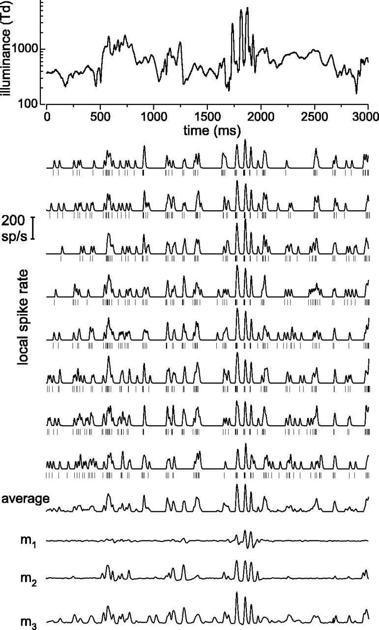
Examples of responses of an on-center MC cell and model responses. The top eight rows of spike rates show eight different responses of the same cell to the stimulus shown at thetop (3 sec of a 10 min stimulus; laboratory environment). The short vertical bars show the timing of individual spikes; local spike rate was estimated here by filtering this spike train with a low-pass filter with a full width at half-maximum of 12.5 msec. Bottom rows show the average of the eight local spike rate traces, the response of a linear model (m₁), the response of a model with a bandpass filter, a compressive nonlinearity, and a rectification (m₂), and the response of the model shown in Figure 7A(m₃). Parameters for modelm₃(see the legend of Fig. 7A) were τ₁ = 6.9 msec, τ₂ = 60 msec, k₁ = 1.2 · 10⁻²td^−1/2, τ₊ = 10 msec,c₁ = 9.5 · 10⁻³,q₀ = 0.57,q₁ = 8.7,c₂ = 1.8 ·  10⁻⁴, τ₃ = 208 msec, and k₂ = 1.1.

Fig. 3.

Examples of responses of a PC and small-bistratified cell, and model responses. The top panel shows the stimulus (overlapping with that of Fig. 2); (l-m)/(l+m) shows the normalized difference of L- and M-cone excitation; (s-0.5(l+m))/(l+m) shows the difference of S-cone excitation and the excitations of the other cones. Thetop four rows of spike rates show responses of a PC cell (+L-M on-center) to this stimulus, with spike trains as in Figure 2; the local spike rate was estimated from the spike trains using a low-pass filter with a full width at half-maximum of 25 msec. Thenext row shows the average of these four responses. Therow marked +L-M/m₃shows the response of the model in Figure7B, with parameters (see the legend of Fig.7B) τ₁ = 6.5 msec, τ₂ = 82 msec, k₁ = 1.7 · 10⁻²td^−1/2, q = 0.07, α = 1.3, k₂ = 32, ando₁ = 0.45. The four rowsmarked +S-ML show responses of a small-bistratified cell, the next row shows their average, and thebottom row (+S-ML/m) shows the response of the model in Figure 7C, with parameters (see the legend of Fig. 7C) τ₁ = 8.0 msec, τ₂ = 60 msec, k₁ = 1.2 · 10⁻²td^−1/2, q₁ = 0.5,q₂ = 0.5, α = 0.5, β = 0.5 , τ₃ = 200 msec,g₁ = 1.28,g₂ = 17,o₁ = −1.5,o₂ = −0.11, γ = 1.3,k₂ = 6.0.

Fig. 8.

Examples of responses of different on-center MC cells. The five top traces show the local spike rate of five different cells, in response to the same section of the stimulus from the laboratory environment as in Figure 2. Bottom traces show average and model prediction. The dashesabove zero (0) show the zero level of the latter two. Model parameters were τ₁ = 8.0 msec, τ₂= 85 msec, k₁ = 8.6 · 10⁻³td^−1/2, c₁ = 1.3 · 10⁻², τ₊ = 8.8 msec, q₀ = 0.52, q₁ = 12.5,c₂ = 3.5 · 10⁻⁴, τ₃ = 283 msec, andk₂ = 1.1.

Information rates can be obtained from normalized spike rates (Brenner et al., 2000); see Equation 12. The spike rate can be calculated as the average response $\overline{\rho }$(t) (Eq. 1), but for small numbers of repeats this will be noisy. Let us assume that, in the frequency domain, the response can be written as r(ω) =p(ω) + ν(ω), with r the Fourier transform of ρ_i(t), p the Fourier transform of the underlying spike rate that we want to estimate, and ν independent noise. The Wiener estimate of p based on the average r̄ of m repeats is thenp = (S_{$\overline{r}$p}/S_{$\overline{r}$$\overline{r}$})$\overline{r}$. The expectation value of the cross-spectrum isS_{$\overline{r}$p} =p², and that of the power spectrum is S_{$\overline{r}$$\overline{r}$} =p² + ν²/m. Therefore, an estimate of p is obtained as:

$$\widehat{p}=\frac{SNR}{SNR+1/m} \overline{r},$$ Equation 10

with the SNR given by Equation 2. Transformingp̂ to the time domain then gives an estimate of the spike rate, η(t), as used in Equation 12. The factor multiplying r̄ in Equation 10 is a low-pass filter. It was smoothed by block averaging with a width proportional to the frequency to prevent fluctuations of the filter at high frequencies affecting the estimate of Equation 12.

RESULTS

Below we give examples of responses of macaque retinal ganglion cells to a CTSI. Next we describe the expected coherence and coherence rate of individual cells, based on repeated stimulus presentations. For the various classes of retinal ganglion cells we then develop models that produce a coherence rate as close as possible to that inferred from response repeatability. Finally, we introduce the concept of a generic cell and proceed to analyze how the retinal cells distribute among themselves information on luminance and chromatic aspects of the stimulus.

Examples of responses

Figure 2 shows responses of an on-center MC cell to a 3 sec stimulus segment from the laboratory environment CTSI. Each response is shown as a spike train (short vertical bars) and, for presentational purposes, as a filtered version that gives an estimate of local spike rate (see Materials and Methods). The average of these local spike rates is also shown. It can be seen, both from the local rates and from the spike trains, that responses are similar but not identical. The traces markedm₁–m₃ are model calculations that will be discussed in a later section.

Examples of responses of a +L-M PC cell and a +S-ML cell are given in Figure 3. The top two panels show the illuminance of the stimulus and two measures of its spectral properties. The four rows marked +L-M give spike trains and local spike rates of the on-center PC cell. The cell responds clearly to increases in the l − mdifference signal. The stretch of stimulus shown was selected to include several such increases, but for the entire time series they were relatively rare. For much of the time, this cell responded mainly to changes in luminance.

The traces marked +S-ML in Figure 3 give responses of an S-cone excitatory cell. This cell responded well to increases ofs relative to l + m and is suppressed when the stimulus shifts to longer wavelengths. The stimulus segment shown was again selected to include large fluctuations of S-cone excitation; when this was low, these cells fired at low rates. They also responded to luminance changes, but in general less vigorously than PC cells.

Coherence and models of individual cells

Expected coherence

From spike trains as in Figures 2 and 3, it was possible to quantify the repeatability of responses, to obtain a measure of the relation of signal to noise, and then to derive the capacity of each neuron to transmit information. Figure4A shows the analysis procedure, which was based on the method of Haag and Borst (1998) for graded potential neurons [see also Borst and Theunissen (1999) and van Hateren and Snippe (2001)]. The averaged response is an estimate of the “signal,” from which the signal power spectrum is calculated. The averaged response is subtracted from each individual response to give a residual that can be considered as “noise.” Averaging the power spectra of these residuals gives an estimate of the noise power spectrum. The SNR is the ratio of signal power spectrum to noise power spectrum. For small numbers of repeats it will be biased because the estimated signal power spectrum will contain some noise power, and the estimated noise power spectrum will contain some signal power. This can be corrected by a bias factor (see Materials and Methods).

A measure of response repeatability, the expected coherence γ ${}_{exp}^2$, follows from γ ${}_{exp}^2$ = SNR/(SNR + 1), assuming noise is additive (Haag and Borst, 1998). Thus γ ${}_{exp}^2$ approaches 1 when the SNR approaches infinity, γ ${}_{exp}^2$ = 0.5 when SNR = 1, and γ ${}_{exp}^2$ = 0 when SNR = 0. A useful quantity that sums the behavior of γ ${}_{exp}^2$ over the frequency domain is the expected coherence rateR_exp (Eq. 4). This is identical, through the equation relating γ ${}_{exp}^2$ and SNR, to Shannon's equation for the information rate in a channel with Gaussian signals and noise, R_inf = ∫log₂(1 + SNR)df. R_exp is therefore expressed in bits/sec. Here neither signals nor noise is Gaussian, thusR_exp cannot be expected to give an unbiased estimate of the information rate (see Information rates, below). To stress this qualification, we use the term “coherence rate” rather than “information rate” forR_exp and related quantities.

The coherence between two signals (here between the “true,” noise-free response and each measured response) quantifies, on a scale of 0–1, how strongly the two signals are (linearly) related for each frequency. If the coherence is 1 at a particular frequency, there is no noise and the frequency components of the two signals can be linearly predicted from one another. Noise will decrease the coherence. A coherence of 0 means the signals are not linearly related at that frequency.

Examples of expected coherence functions are shown in Figure4B for several cell classes and for both CTSIs. Note that the coherence functions shown here and below have inherent low-pass characteristics (see Materials and Methods); no explicit low-pass filtering on the raw spike trains was used here. Coherences of MC cells (such as the on-center cell shown) were larger and extended to higher frequencies than those of PC cells (such as the +L-M on-center cells) and the small-bistratified cells (+S-ML cells). Coherences obtained with the flower show CTSI are higher than those obtained with the laboratory environment CTSI. The former are close to zero above 75 Hz, because of the limitation of the frame rate of the display (150 fps). Although the coherence of MC cells stimulated with LEDs driven at 400 samples per second (laboratory environment) extends to frequencies >100 Hz, it is low for frequencies above 75 Hz. This suggests that the frame rate of the display used for the flower show stimulus does not strongly limit the coherence rates obtained with this stimulus. The coherence rates corresponding to the coherence functions in Figure 4B are 55 and 114 bits/sec for the two CTSIs for the on-center MC cells, 12 and 39 bits/sec for the +L-M cells, and 32 and 55 bits/sec for the +S-ML cells.

Model development and optimization

Coherence functions and coherence rates can also be obtained between the stimulus and the response. For Gaussian signals and noise, the coherence rate between stimulus and response is identical to the information rate derived from the stimulus reconstruction method described by Bialek et al. (1991) and formulated in the frequency domain by Theunissen et al. (1996). The coherence is the cross-power spectrum of the two signals normalized by their power spectra. Here we do not reconstruct the stimulus from the response but construct the response from the stimulus. We also extend the analysis to include nonlinear models; Figure 5 shows the method (van Hateren and Snippe, 2001). A nonlinear model transforms the stimulus into a signal s_mod. The Wiener filter is the optimal constructing filter as defined in Equation9. Computing the coherence γ² and coherence rate R_coh = −∫log₂(1 − γ²)df betweens_mod and an actually measured responser then quantifies how well the model performs compared with the real system (the retinal ganglion cell).

Ideally, the model should perform as does the cell itself. The performance of the cell itself was quantified above, namely as its expected coherence rate, R_exp, i.e., the expectation value of the coherence rate between the “true” response of the cell (i.e., without noise) and actually measured responses. We can thus adopt the following strategy (van Hateren and Snippe, 2001) for finding an adequate model. The parameters of a particular model are varied to maximize its coherence rateR_coh with the responses of a particular cell. This is compared with the expected coherence rateR_exp of the same cell. IfR_coh is systematically smaller thanR_exp for a particular class of ganglion cells, the model needs to be amended. Amendments are then made, and they are accepted if they bringR_coh (after maximizing again) closer to R_exp. The type of amendments needed can often be inferred from a comparison of expected and model coherence functions, and of the response r and the constructed response r′ (Fig. 5), but much of the model optimization is a process of trial and error.

Figure 6 illustrates for an MC on-center cell how increasingly complex models approach the expected coherence function (thick line, R_exp= 55 bits/sec). Responses r′ constructed with these models are shown in Figure 2, with the same low-pass filter used to derive local spike rates. Model m₁ is a straightforward linear model (i.e., the Wiener filter alone), and its coherence falls far short of the expected value (Fig. 6); the corresponding coherence rate, R_coh, was 8.5 bits/sec. The first problem of a linear model is that it ignores the rectification of the signal, which is marked in MC cells. Model m₂ is an attempt to take this into account. It consists of a low-pass filter (Fig.7A,LP₁), a high-pass filter (as in Fig.7A, with q fitted to a fixed value), a compressive nonlinearity (Fig. 7A,NL₂), and a rectification. Although this model performs much better than m₁ (Fig.6), R_coh = 31 bits/sec is still appreciably smaller than R_exp (55 bits/sec). As trace m₂in Figure 2 shows, the responses to large “on” transients in the stimulus are now well accounted for, but small transients are missed. There are two mechanisms that repair this deficiency. First, a luminance gain control module helps to enhance response to small luminance variations embedded in regions where the average luminance is low. Adding the luminance gain control shown in Figure 7Aincreases R_coh to 35 bits/sec for this cell. Second, model m₂does not saturate at high contrasts, i.e., it lacks a contrast gain control module. The most satisfactory model found so far, which includes a contrast gain control module, m₃, is shown in Figure 7A and gave aR_coh = 42 bits/sec. Although this is still smaller than R_exp, it accounts for approximately three-quarters ofR_exp in this particular cell.

Fig. 7.

Models for retinal ganglion cells.A, Model for the MC cells.I_i is the retinal illuminance; LP₁is a low-pass filter consisting of a cascade of three first-order filters, each with time constant τ₁;LP₂is a first-order low-pass filter with time constant τ₂;NL₁is a nonlinearity of the form output = (2/π)atan(k₁ · input);LP_qis a low-pass filter of a form that makes the entire feedforward loop behave as a high-pass filter with a frequency-domain slope q (Snippe et al., 2000), where q is given by the output ofLP₃; LP₊has time constant τ₊;NL₊is output = (1 + rec₊(input)/c₁)², with rec₊ an operator that half-wave rectifies, retaining only the positive values of its input; (…) ${}_{\text{c}+}^2$squares its half-wave rectified input, retaining positive signals for on-center MC cells and negative signals for off-center MC cells, in both cases related to positive luminance changes;NL_cis output =q₀ +q₁ · input/(c₂+ input); LP₃has a time constant τ₃;NL₂is output = (2/π)atan(k₂ · input).B, Model for +L-M and −M+L PC cells; models for -L+M and +M-L cells are given by interchanging theI_LandI_Mat the input.I_LandI_Mare the effective L- and M-cone illuminances, for the CTSIs equal to l andm (see Materials and Methods);LP₁,LP₂,NL₁, andNL₂are as defined atA; LP_qis similar to LP_qat A, with q not variable.C, Model for the +S-ML cell.I_sis the S-cone illuminance, for the CTSIs equal to s;LP₁,LP₂, andNL₁as defined atA; LP_q1and LP_q2are similar to the LP_qat A, with q₁and q₂ not variable;LP₃has time constantτ₃;NL₂is output =g₁· atan(g₂ · input);NL₃is output = (2/π)atan(k₂ · input).

It should be noted that Figure 7A shows only that part of the MC cell model preceding the Wiener filter (as in Fig. 5). Theinset in Figure 6 shows the impulse response of the Wiener filter of this cell with model m₃, with the horizontal line in front designating the zero level, and a time scale of 50 msec. The fact that the Wiener filter is here essentially a simple low-pass filter suggests that the model itself incorporates most of the required filtering (both linear and nonlinear). For example, the biphasic impulse responses of MC cells (Lee et al., 1994) are produced mainly by the high-pass filter in the model.

Models of retinal ganglion cells

We first developed models for all ganglion cell types from which we recorded. The model for the MC cells was represented in Figure7A (a sign change half-way into the model provides a signal inversion for off-center cells). The model derives primarily from results from the literature. It assumed that MC cells receive summed input from L- and M-cones in a ratio of 1.6:1. The model consists of an initial luminance gain control (Lankheet et al., 1993; Snippe et al., 2000; Smith et al., 2001), followed by a compressive nonlinearity. These may represent outer retinal mechanisms. There follows a high-pass filter. The high-pass filter is implemented here as having a power-law slope (with power q) of its transfer function [see Snippe et al. (2000) for a discussion of this type of filter]. The model required a fast and a slow contrast gain control. The fast one (the inner loop) is a divisive feedback of positive peaks in the response, essentially making peaks sharper and reduced in area. The nonlinearity (NL₊) is expansive, which means that large peaks are affected more strongly than small peaks. We found that adding a similar control on negative-going signals did not changeR_coh, and therefore we omitted it. In principle, this element resembles the contrast gain control mechanism described for cat ganglion cells (Victor, 1987). The slow contrast gain control (the outer loop) controls, through a nonlinearity and a low-pass filter, the slope (q) of the high-pass filter. The input module of this loop, (…) ${}_{\text{c}+}^2$, uses only signals related to increases in the luminance of the stimulus, i.e., positive signals for on-center MC cells, and only negative signals for off-center MC cells. Note that the gain control at the front end of the model retains some dependence on luminance in its output [it falls short of Weber's law (Smith et al., 2001)]. This also applies to the other modules leading to the input of the outer control loop. Therefore, this loop may relate to inner retinal gain controls that modify the time course of MC cell responses as a function of luminance (Lee et al., 1994). Finally, the model contains a compressive nonlinearity and a rectification. We found that none of the modules in Figure 7A can be omitted; all contribute significantly toR_coh.

We expanded the MC model to contain separate luminance gain controls for the L- and M-pathways, which were then added with a weightingw_L for the L-signal and (1-w_L) for the M-signal. This revealed that the weighting w_L varied substantially from cell to cell (ranging from 0 to 1; mean ± SD was 0.67 ± 0.28), as reported elsewhere (Valberg et al., 1992). However, this increased R_coh only marginally (by ∼1.5%). This shows that it is justified to treat MC cells as luminance-driven cells, at least for naturalistic stimuli, and that information processing by MC cells appears mostly independent of whether they derive their main input from L- or M-cones.

We tried several other models or functional modules published in the literature (Victor, 1987; Wilson, 1997), but none performed as well as the model in Figure 7A. However, our purpose was not to compare candidate models but to derive a relatively simple model that captures the responses of ganglion cells to our stimuli, such that we can use these models for analysis of visual coding by these neurons. It should thus be considered as a descriptive approach, which does not claim to precisely represent the underlying physiology. However, the luminance and contrast gain control modules closely resemble suggestions in the literature.

The model for the PC cells (Fig. 7B) contains initial separate gain controls and compressive nonlinearities for the L- and M-cone pathways. These may again correspond to outer retinal mechanisms. It was then necessary to provide a low-pass-filtered luminance signal subtracting from the L- and M-cone pathways (consistent with producing a power-law high-pass filter). After subtraction of cone signals (i.e., the cone opponent stage), a compressive nonlinearity, an offset, and a rectification complete the model. Note that no further gain controls are necessary for this cell type, which is consistent with other data from the literature (Benardete et al., 1992; Yeh et al., 1995).

The model for the S-cone excitatory cell proved to be the least successful of those developed here. One of the problems is a slow adaptation phenomenon, in which after prolonged absence of short-wavelength components in the stimulus the cell does not immediately respond when they reappear, but only after a variable delay. We modeled this as a variable threshold (Fig. 7C), with a slow filter LP₃. The top pathway in Figure 7C is a +S-cone pathway. Thebottom pathway is a long-wavelength opponent pathway (L+M).

Expected and model coherence rates of retinal ganglion cells

Expected coherence rates and model coherence rates were evaluated for several models and all ganglion cells for which there was sufficient data; fits were made separately for each individual cell. The results are shown in Table 1 for both CTSIs used. The results show that, as remarked above,R_exp is larger for MC cells than for PC cells, with +S-ML cells lying in between. The flower show stimulus gives higher coherence rates than the laboratory environment (see Discussion). As shown in Table 1 for MC on-center, MC off-center, and +L-M on-center cells (similar results were obtained for the other cell types), purely linear models (m₁) that add cone signals do not work well. Model m₂ for the +L-M cell is a linear opponent model; it performs better than m₁, but not as well as the full model (m₃) of Figure 7B. The best models we found capture 60–70% of the expected coherence rate of MC cells, 80–90% for PC cells, and ∼50% for +S-ML cells.

Table 1.

Coherence rates of individual cells

Cell type (number of cells)	Rexp(bits/sec)	Rcoh (bits/sec)		Average Rcoh/ Rexp
Laboratory environment
MC on-center (5)	51  ± 17	m1	8  ± 2	0.17  ± 0.04
		m2	24  ± 8	0.48  ± 0.10
		m3	33  ± 12	0.65  ± 0.13
MC off-center (4)	50  ± 20	m1	7  ± 2	0.14  ± 0.04
		m2	23  ± 6	0.47  ± 0.12
		m3	32  ± 8	0.68  ± 0.17
+L−M on-center (5)	13  ± 3	m1	4  ± 2	0.33  ± 0.17
		m2	9  ± 3	0.66  ± 0.21
		m3	12  ± 4	0.96  ± 0.21
−L+M off-center (2)	5  ± 1	5 ± 1		0.91
+M−L on-center (5)	14  ± 5	10 ± 5		0.74  ± 0.14
−M+L off-center (1)	9	8		0.91
+S−ML (4)	27  ± 10	14 ± 3		0.53  ± 0.10
Flower show
MC on-center (3)	108  ± 6	m1	21  ± 2	0.19  ± 0.01
		m2	49  ± 2	0.45  ± 0.01
		m3	71  ± 3	0.66  ± 0.04
MC off-center (1)	74	m1	17  ± 1	0.23  ± 0.01
		m2	37  ± 4	0.51  ± 0.05
		m3	48  ± 1	0.65  ± 0.02
+L−M on-center (3)	46  ± 7	m1	24  ± 4	0.53  ± 0.06
		m2	27  ± 4	0.59  ± 0.06
		m3	39  ± 5	0.85  ± 0.06
−L+M off-center (2)	23  ± 4	21 ± 2		0.90  ± 0.05
+M−L on-center (1)	45	37 ± 2		0.81  ± 0.03
−M+L off-center (2)	25  ± 1	17 ± 3		0.68  ± 0.13
+S−ML (3)	55  ± 26	24 ± 6		0.47  ± 0.10

For the MC cells, m₁ is a linear model; m₂ is a model containing a low-pass filter (LP₁ in Fig. 7A), a fixed high-pass filter (fixed q in Fig. 7A), a compressive nonlinearity (NL₂ in Fig. 7A), and a rectification; m₃ is the full model of Figure7A. For the on-center +L−M cell, m₁ is a linear model; m₂ is a model containing a weighted subtraction ofl and m; and m₃ is the full model of Figure 7B. For the other M, L-cells, the model is given in Figure 7B; for the +S−ML cell the model is given in Figure7C. Numbers show mean and SD. Fits were made separately for each cell.

Coherence and models of generic cells

Responses of an individual neuron to the same stimulus are variable (Figs. 2, 3). The responses of different neurons of the same class show further variability. Figure 8shows responses of five different on-center MC cells to the same stimulus. There are differences that exceed the variability of the responses of an individual neuron. Thus, for a uniform field, the information delivered to the cortex by the array of on-center MC cells, for instance, is slightly different for each cell of the array, even for cells of similar eccentricity (as was the case here).

There are two possibilities as to how the cortex might deal with this variability. Either it knows (or learns) the temporal characteristics of each individual neuron and uses all information in the signal of each cell, or it considers the variability between neurons as a source of (structural) noise that should be neglected. Then, it should base its analysis on the characteristics that all neurons of a particular class have in common. Although the first possibility was implicit in the above attempt to develop a model that optimally described individual neurons, we now analyze the second possibility. It leads to the concept of a generic neuron, which represents its class of neurons, and produces a response around which the responses of individual neurons are distributed. We will study these generic neurons in the simplest way possible by treating the responses coming from different neurons (of one class) as if they were generated by a single generic neuron. We can then use the same methods and calculate the expected coherence rate, now of the generic neuron, and evaluate the coherence rate of the various models describing the generic cell.

Figure 9 shows the expected coherence of a group of responses obtained from different on-center MC cells. The coherence between measurements and model response [(Fig.7A, light trace) with m₃the same model as used for the on-center MC cell above] is close to the expected coherence. The coherence rates in this example areR_exp = 21 bits/sec andR_coh = 20 bits/sec. The remaining discrepancy is at frequencies in the range 0–10 Hz, but it is small. The inset again shows the Wiener filter following the nonlinear model.

We performed an analysis of generic neurons for all cell classes; the results are given in Table 2. Table 2shows that again R_exp is larger for MC cells than for PC cells, and there are again higher coherence rates for the flower show than for the laboratory environment. Because of the additional intercell variability, all rates are lower than the result for individual neurons in Table 1. Models typically capture ∼90% of the expected coherence rates.

Table 2.

Coherence rates of generic cells

Cell type (number of cells)	Rexp(bits/sec)	Rcoh (bits/sec)		Average Rcoh/ Rexp
Laboratory environment
MC on-center (5)	21.3  ± 1.4	m1	6.4  ± 0.3	0.30  ± 0.03
		m2	15.6  ± 1.1	0.73  ± 0.06
		m3	19.7  ± 1.3	0.93  ± 0.07
MC off-center (4)	16.3  ± 0.9	m1	4.9  ± 0.2	0.30  ± 0.02
		m2	13.8  ± 0.7	0.85  ± 0.06
		m3	17.2  ± 1.2	1.05  ± 0.07
+L−M on-center (5)	4.5  ± 0.6	m1	1.8  ± 0.4	0.40  ± 0.07
		m2	3.3  ± 0.8	0.73  ± 0.19
		m3	4.9  ± 0.9	1.09  ± 0.22
−L+M off-center (2)	3.9	3.6		0.92
+M−L on-center (5)	7.0  ± 0.5	7.2 ± 1.6		1.04  ± 0.23
−M+L off-center (1)
+S−ML (4)	10.3  ± 3.1	7.3 ± 1.6		0.73  ± 0.18
Flower show
MC on-center (3)	63  ± 4	m1	19  ± 1	0.30  ± 0.02
		m2	41  ± 1	0.65  ± 0.05
		m3	55  ± 2	0.89  ± 0.07
MC off-center (1)
+L−M on-center (3)	40  ± 1	m1	22  ± 1	0.56  ± 0.02
		m2	25  ± 1	0.63  ± 0.02
		m3	35  ± 1	0.88  ± 0.03
−L+M off-center (2)	20  ± 1	18 ± 1		0.92  ± 0.05
+M−L on-center (1)
−M+L off-center (2)	18  ± 1	16 ± 1		0.88  ± 0.07
+S−ML (3)	19  ± 2	17 ± 1		0.91  ± 0.13

Coherence rates show averages and SD for calculations for each of six repeats of the stimulus to each cell. Models are as described in the legend of Table 1. Fits were made simultaneously to all cells from a particular class but separately for the two different stimuli.

In the above analysis we pooled all recorded neurons from a particular class, regardless of whether they were measured in the same animal, although in principle, intercell variability may be smaller within an animal than between animals. We therefore compared interanimal and intra-animal variability in coherence rates. Interanimal variability was slightly larger than the intra-animal variability, but the difference was small compared with the overall reduction in coherence rate in generic cells.

Behavior of compound cells

In an abstract sense, the retina can be considered as a device that transforms the stimulus into different representations. We wished to analyze what these representations encode. To simplify notation, we use the following abbreviations: M_on for the on-center MC cell, M_off for the off-center MC cell, R_on for the +L-M on-center PC cell, R_off for the −L+M off-center PC cell, G_on for the +M-L on-center PC cell, G_off for the −M+L off-center PC cell, and B_on for the +S-ML cell. For the generic models developed in the previous section the notation is, e.g.,M̂_on, where the circumflex indicates that we are dealing with the output of a generic model.

As a first analysis step, we combine on- and off-cells into compound cells by subtracting measured responses (i.e., spike trains) of on- and off-center cells belonging to a corresponding class. For example, the M_o compound cell is defined as M_o = M_on − M_off . Similarly, we define R_o = R_on − R_off and G_o = G_on − G_off . Because measurements on the −S+LM cell are lacking, for the short-wavelength pathway we used B_on. We can define the analogs for the generic models. Thus M̂_o =M̂_on − M̂_off, and so on.

By combining measurements from the available M_onand M_off cells, a large number of responses of M_o are constructed. The coherence rate between each of the M_o responses and the generic model response M̂_o is subsequently calculated and averaged over all M_o responses. The result is shown in the top left entry of Table 3. It is a measure of how much an M_o response tells about the response of model M̂_o, and therefore also a measure of how much it tells about the stimulus. Similarly, the second entry in the top row of Table 3 shows the coherence rate between measured M_o responses and the R̂_o model. It shows that the M_o responses are less coherent with theR̂_o model than with theM̂_o model, but the difference is not large. A similar conclusion follows from the coherence rates between measured R_o responses and theM̂_o model or theR̂_o model (second row in the Table). The correspondence between various compound cells can be quantified by defining the cross-coherence coefficient,r_cc. For example, for M_o and R_o it is defined as:

$$r_{\text{cc}}={\left[\frac{R_{\text{coh}}(M_{\text{o}},{\widehat{R}}_{\text{o}})R_{\text{coh}}(R_{\text{o}},{\widehat{M}}_{\text{o}})}{R_{\text{coh}}(M_{\text{o}},{\widehat{M}}_{\text{o}})R_{\text{coh}}(R_{\text{o}},{\widehat{R}}_{\text{o}})}\right]}^{1/2},$$ Equation 11

with M_o, M̂_o, R_o, and R̂_odefined as above. It essentially gives the ratio of two coherence rates, one of measurements with the generic model of another compound cell and one with their own generic model. If the coherence rate of the measurements with the other model is zero,r_cc is zero as well, whereasr_cc = 1 if the coherence rates of the measurements with the other and their own model are equal. Thusr_cc is expected to vary between 0 and 1 depending on how much the two sets of measurements/generic models have in common.

Table 3.

Coherence rates and cross-coherence coefficients of compound cells

R_coh and r_cc for {M_o, R_o, G_o, B_on}

Rcoh	M̂o	R̂o	Ĝo	B̂on
Mo	69  ± 4	48  ± 3	36  ± 1	7.9  ± 0.4
Ro	29  ± 5	39  ± 5	22  ± 4	4.6  ± 0.9
Go	25  ± 2	20  ± 1	33  ± 4	7.0  ± 0.5
Bon	5.3  ± 2.7	4.5  ± 2.5	5.1  ± 2.7	18  ± 5
rcc	M̂o	R̂o	Ĝo	B̂on
Mo	1	0.72  ± 0.12	0.63  ± 0.07	0.18  ± 0.07
Ro	0.72  ± 0.12	1	0.60  ± 0.10	0.17  ± 0.08
Go	0.63  ± 0.07	0.60  ± 0.10	1	0.24  ± 0.11
Bon	0.18  ± 0.07	0.17  ± 0.08	0.24  ± 0.11	1
Rcohand rcc for {Mo, Pa, Pc, Bon}
Rcoh	M̂o	P̂a	P̂c	B̂on
Mo	69  ± 4	49  ± 2	9.5  ± 1.4	7.9  ± 0.4
Pa	41  ± 2	51  ± 3	6.6  ± 0.8	5.6  ± 0.7
Pc	1.5  ± 1.2	1.9  ± 1.1	10.5  ± 1.8	0.9  ± 0.3
Bon	5.3  ± 2.7	5.1  ± 2.9	1.4  ± 0.7	18  ± 5
rcc	M̂o	P̂a	P̂c	B̂on
Mo	1	0.77  ± 0.05	0.14  ± 0.08	0.18  ± 0.07
Pa	0.77  ± 0.05	1	0.15  ± 0.07	0.20  ± 0.09
Pc	0.14  ± 0.08	0.15  ± 0.07	1	0.08  ± 0.04
Bon	0.18  ± 0.07	0.20  ± 0.09	0.08  ± 0.04	1

Compound cells are defined as M_o = M_on − M_off, R_o = R_on − R_off, G_o = G_on − G_off, P_a = R_o + G_o, P_c = R_o − G_o.

The coherence rates for all compound cells, and the correspondingr_cc values, show that there is appreciable overlap between information carried in the magnocellular channel (M_o) and the two M-, L-cone opponent channels (R_o and G_o), but much less with the S-cone cells (B_on). It also shows that the R_o and G_ocompound cells overlap. It is likely that the overlap between M_o, R_o, and G_o is caused by the fact that all of these compound cells respond to changes in luminance. We now ask if it is possible, for R_o and G_o, to separate the response component (and coherence rate) related to luminance from that related to chromaticity. A simple scheme is to combine R_o and G_o in two different ways: P_a = R_o + G_o and P_c = R_o − G_o. Here, in theory, P_ashould respond only to achromatic and not to chromatic aspects of the stimulus, whereas P_c should respond, again in theory, only to chromatic and not to achromatic aspects of the stimulus. This scheme resembles a time-domain version of the demultiplexing scheme for cortical processing of the PC pathway (Lennie and D'Zmura, 1988). Note that we are not proposing here that P_a and P_c are actually constructed centrally; we use P_a and P_c only as a convenient way to separate and study the luminance and chromaticity related information in the set of PC cells.

The bottom part of Table 3 shows the result of this transformation. It shows that although P_a and M_o are still strongly related, P_c and B_on are now only loosely related to both M_o and P_a, and also to each other. From the coherence rates of P_a with P̂_aand P_c with P̂_c, it can be seen that, for this particular stimulus (the flower show), the parvocellular channel has a coherence rate for luminance that is approximately five times larger than that for chromaticity. The four neurons constituting the P_c channel together have a coherence rate that is only approximately one-half the coherence rate of the single-cell B_on channel.

The coherence rates of M_o, P_a, P_c, and B_on in Table 3 are integrations over frequency of (transforms of) the respective coherence functions (Eq. 8). It is instructive to look at the coherence functions themselves, to see how they vary with frequency. Figure 10shows that the chromatic channels P_c and B_on are confined to relatively low temporal frequencies, with B_on mostly above P_c. M_o continues to somewhat higher frequencies than P_a, and the two cells constituting M_o have, over much of the frequency domain, a coherence higher than that of the four cells constituting P_a. Only at very low frequencies does P_a have a higher coherence (i.e., a higher SNR) than M_o. Much of this is consistent with the power spectra of the average of all cell recordings for M_o (denoted by $\overline{M}$_o), P_a, P_c, and B_on (Fig. 11). For example, for frequencies smaller than a few Hz, $\overline{P}$_a has considerably more power than $\overline{M}$_o.

Fig. 10.

Coherence between compound cell responses and compound cell models. Compound cells are defined as a magnocellular M_o = M_on − M_off, an achromatic parvocellular P_a = R_o + G_o, with R_o = R_on− R_off and G_o = G_on − G_off, a chromatic parvocellular P_c= R_o − G_o, and the S-cone-driven B_on. The coherence functions are the average of the coherence calculated for all recorded responses from all cells. Parameters were as follows: on-center MC cell (M_on): τ₁ = 6.0 msec, τ₂ = 47 msec,k₁ = 1.8 · 10⁻²td^−1/2, c₁ = 2.0 · 10⁻², τ₊ = 2.0 msec, q₀ = 0.19, q₁ = 20,c₂ = 5.4 · 10⁻⁴, τ₃ = 104 msec, k₂ = 0.62; off-center MC cell (M_off): τ₁ = 5.5 msec, τ₂ = 40 msec,k₁ = 3.1 · 10⁻³td^−1/2, c₁ = 1.1 · 10⁻³, τ₊ = 12 msec, q₀ = 0.06, q₁ = 2.1,c₂ = 2.0 · 10⁻⁵, τ₃ = 171 msec, k₂ = 0.15; +L-M on-center (R_on): τ₁ = 4.3 msec, τ₂ = 221 msec,k₁ = 2.3 · 10⁻²td^−1/2, q = 0.71, α = 0.08, k₂ = 0.61,o₁ = −1.0 · 10⁻³; -L+M off-center (R_off): τ₁ = 6.7 msec, τ₂ = 79 msec, k₁ = 8.5 · 10⁻²td^−1/2, q = 0.32, α = 0.49, k₂ = 6.1,o₁ = 0.22; +M-L on-center (G_on): τ₁ = 5.7 msec, τ₂ = 129 msec, k₁ = 6.2 · 10⁻²td^−1/2, q = 0.04, α = 0.67, k₂ = 2.3,o₁ = −4.4 · 10⁻³; -M+L off-center (G_off): τ₁ = 5.1 msec, τ₂ = 26 msec, k₁ = 2.0 · 10⁻²td^−1/2, q = 0.08, α = 2.6, k₂ = 2.2,o₁ = 6.5 · 10⁻³; +S-ML cell (B_on): τ₁ = 8.0 msec, τ₂ = 60 msec,k₁ = 3.4 · 10⁻²td^−1/2, q₁ = 0.5,q₂ = 0.5, α = 0.5, β = 0.5, τ₃ = 200 msec,g₁ = 0.61,g₂ = 134,o₁ = −1.06,o₂ = −0.37, γ = 0.36, andk₂ = 0.38.

Fig. 11.

Power spectra of compound cell responses. The spike trains of all recorded responses of all cells belonging to a particular class were averaged and combined to form the compound cells defined as in Figure 10. Without low-pass filtering, the power spectra of these averages were calculated. Higher frequencies in the spectra are smoothed (averaged with a group of neighboring frequencies, with the group size proportional to frequency).

Information rates

For independent Gaussian signals and noise the coherence rate is identical, from Shannon's equation, to information rate (Haag and Borst, 1998; van Hateren and Snippe, 2001). In our case neither signals nor noise is Gaussian, and it remains unclear how different the coherence rates are from the true information rates. We therefore compared the coherence rates with an independent estimate of information rate that does not depend on assuming independent Gaussian signals and noise. One such estimate, neglecting possible information in complex spike patterns (Brenner et al., 2000; Reinagel and Reid, 2000), is:

$$R_{\text{inf}}=\frac{1}{T}\underset{0}{\overset{T}{\int }} \text{dt} \eta (t){log}_2(\eta (t)/\overline{\eta }),$$ Equation 12

(Brenner et al., 2000), where η(t) is the spike rate as a function of time, $\overline{\eta }$ is the average spike rate, andT is the duration of the response to be analyzed. Because in our case the number of repeats is small (6 for individual cells, up to 30 for generic cells), it is crucial to decide on the time resolution (bin size) of the spike rate estimate. If the bin size is too small, η(t) is very noisy, which will lead to overestimatingR_inf. If it is too large, real structure in η(t) is lost, which will lead to underestimating R_inf. To avoid arbitrariness in the choice of time resolution, we followed the following procedure. First we collected a poststimulus time histogram with small bin sizes (here 1 msec, but the exact value is not crucial for the results). Subsequently, this histogram was filtered with the optimal Wiener filter to obtain an estimate of the spike rate, η(t) (see Materials and Methods; Eq. 10). The Wiener filter strongly reduces noisy high-frequency components in the raw histogram, which would otherwise upwardly bias the estimate ofR_inf with Equation 12. An adverse effect of the Wiener filter is that it may also reduce signal components of the neurons, and thus downwardly bias the estimate ofR_inf. The latter effect is in fact limited. We investigated this by varying the number of repeats,m, used for the estimate ofR_inf, and computing the frequency,f_c, where the amplitude of the Wiener filter drops to 50% of its maximum. The estimate ofR_inf depends only mildly on the number of repeats, being 10–15% larger at m = 6 than atm = 2. The bandwidth of the Wiener filter is such that it encompasses much of the signal bandwidths of the cells; for all cells measured, the coherence rate obtained by integrating up tof_c(f₀ =f_c in Eq. 4) is close to 90% of the total coherence rate. The Wiener filter is therefore unlikely to strongly bias R_inf. Another source of bias in the estimated information rates, neglecting information in complex spike patterns, is limited in another mammalian species, cat (Reinagel and Reid, 2000). We conclude that the information rates we present here are most likely accurate at least within a factor of 2.

Table 4 gives the results of this analysis, for both types of CTSIs, and for both individual and generic neurons. It also summarizes the average spike rates that we measured in the various classes of ganglion cells with these stimuli and the average bits per spike. Finally, it compares the information rates obtained from Equation 12 with the coherence rates as presented in Tables 1 and 2.

Table 4.

Information rates

Cell type (number of cells)	Rinf(bits/sec)	Spike rate (spikes/sec)	Bits/spike	Rexp(bits/sec)	Rinf/ Rexp
Individual cells–laboratory environment
MC on-center (5)	29  ± 5	34  ± 6	0.9  ± 0.3	51  ± 17	0.57
MC off-center (4)	29  ± 14	36  ± 14	0.8  ± 0.2	50  ± 20	0.59
+L−M on-center (5)	8.3  ± 2.1	27  ± 20	0.6  ± 0.6	13  ± 3	0.64
−L+M off-center (2)	3.2  ± 2.0	26  ± 3	0.1  ± 0.1	5  ± 1	0.65
+M−L on-center (5)	9.8  ± 5.2	24  ± 19	0.7  ± 0.6	14  ± 5	0.70
−M+L off-center (1)	10	19	0.5	9	1.11
+S−ML (4)	18  ± 10	32  ± 4	0.6  ± 0.3	27  ± 10	0.67
Individual cells–flower show
MC on-center (3)	72  ± 21	43  ± 16	1.8  ± 0.3	108  ± 6	0.67
MC off-center (1)	45	54	0.8	74	0.61
+L−M on-center (3)	30  ± 6	33  ± 8	0.9  ± 0.1	46  ± 7	0.66
−L+M off-center (2)	16  ± 3	40  ± 15	0.5  ± 0.3	23  ± 4	0.71
+M−L on-center (1)	30	32	0.9	45	0.66
−M+L off-center (2)	21  ± 1	32  ± 4	0.7  ± 0.1	25  ± 1	0.83
+S−ML (3)	28  ± 10	23  ± 13	1.5  ± 1.0	55  ± 26	0.51
Generic cells–laboratory environment
MC on-center (5)	21	34	0.6	21  ± 1	1.00
MC off-center (4)	19	36	0.5	16  ± 1	1.17
+L−M on-center (5)	4.4	27	0.2	4.5  ± 0.6	0.98
−L+M off-center (2)	2.7	26	0.1	3.9	0.70
+M−L on-center (5)	8.4	24	0.4	7.0  ± 0.5	1.20
−M+L off-center (1)
+S−ML (4)	12.9	32	0.4	10  ± 3	1.25
Generic cells—flower show
MC on-center (3)	67	43	1.6	63  ± 4	1.07
MC off-center (1)
+L−M on-center (3)	30	33	0.9	40  ± 1	0.74
−L+M off-center (2)	16	40	0.4	20  ± 1	0.79
+M−L on-center (1)
−M+L off-center (2)	19	32	0.6	18  ± 1	1.10
+S−ML (3)	21	23	0.9	19  ± 2	1.13

R_inf shows the information rate obtained with Equation 12; bits/spike shows the information per spike, and R_exp is the coherence rate as also given in Tables 1 and 2.

As can be seen in Table 4, information in terms of bits per spike is typically between 0.5 and 1, which is similar to values reported for other spiking neurons (Borst and Theunissen, 1999). Values in MC cells tend to be slightly higher than those in PC cells.

The last column of the table shows the ratio of the information rate and coherence rate. Although this ratio is typically 60–70% for individual neurons, it distributes around 100% for generic neurons. One reason for the lower values for individual neurons is the smaller number of repeats (6) available, which will tend to underestimateR_inf somewhat more than for the generic neurons (12–30 repeats). A second reason may be that the coherence rate systematically overestimates the true information rate because the assumptions of Shannon's equation are not fully met; signals and noise are not Gaussian. Furthermore, it is assumed for Shannon's equation that all temporal frequencies in the response are independent from one another. This may not be the case here: nonlinearities can produce correlations between different frequencies (in particular, harmonics of each other). These correlations will lead to overestimation of the information rate. This effect may be greater for individual neurons than for generic neurons, because the coherence functions of the former extend over a larger range of frequencies, and individual cells appear to display more marked, cell-specific nonlinearities than is apparent from generic responses.

Nevertheless, Table 4 shows that the coherence rates are of the same order of magnitude as the information rates, both for individual and for generic neurons.

DISCUSSION

The primate retina provides the sole input to central visual mechanisms, through a well defined set of receptors and cell arrays. We have investigated how information is distributed among these arrays when natural temporal stimuli are presented to the retina. Chromatic information in the PC channel is confined to low temporal frequencies (Fig. 10). Even for the particularly colorful stimuli used here, this channel carries approximately five times less information in the chromatic than in the achromatic domain (Table 3). Information in the S-cone-driven ganglion cells is also confined to low temporal frequencies. Information in the MC pathway extends to higher frequencies than the achromatic component of the PC channel signal, but the MC pathway transmits less signal power than in the PC channel for frequencies below 2–3 Hz (Fig. 11).

PC cells show much greater cone contrast sensitivity to chromatic than to luminance modulation (Lee et al., 1993). The dominant weighting of achromatic stimulus components in determining their response to natural environments is attributable to the high achromatic contrast in a natural scene, whereas the chromatic contrast associated with the  L-M  signal is much smaller (Fig. 1F) (Ruderman et al., 1998).

The present study analyzes the representation of the information present in the retinal output, but this provides no evidence as to how far this information is used at higher stages of visual processing. Nevertheless, several results of the analysis can be related to earlier studies (Lee et al., 1990). That study showed that responsivity of MC cells to luminance modulation matches human detection performance well for frequencies up to 20 Hz. At higher frequencies, the responsivity of individual MC cells exceeds the sensitivity of human observers. A similar difference in frequency range is seen here when comparing the expected coherence function of an individual MC cell (Fig. 6) with that of the generic MC cell (Fig. 9). This may offer a functional explanation for the difference between psychophysical and physiological performance; although individual MC cells have a good SNR over a broad frequency range, the set of MC cells participating in the psychophysical response gives incoherent responses at high frequencies. Rather than extracting information from the variable behavior of individual cells at high frequencies (which might be computationally expensive), these frequencies may be ignored for the psychophysical decision (e.g., by filtering them out through a cortical low-pass filter) (Lee et al., 1990).

The chromatic component of the generic PC cell response has a coherence function limited to low frequencies. Psychophysical detection of chromatic modulation is restricted to a similar frequency range, despite the fact that individual PC cells respond to higher frequencies. This again requires postulation of central low-pass filtering of chromatic channels (Lee et al., 1990). The restricted frequency range of the generic PC cell chromatic coherence function is most likely attributable to the properties of the CTSI. As Figure1F shows, the chromatic contrast of the  L-M  signal is low compared with achromatic contrast and declines further with frequency. Additive noise in the retina may then lead to low SNRs already for quite low frequencies. Thus the restricted frequency range in psychophysical performance could be an adaptation of central filters to match the frequency range from which the  L-M  system can obtain useful information on the visual environment. Low-pass filtering of PC cell signals is unlikely to be modality specific, so that the PC cell achromatic coherence above 10 Hz (Fig. 10) may not be used centrally. Relevant cortical measurements are unavailable.

We developed models for the various retinal ganglion cell classes. Linear models did not work well, mainly because the intensity range is too large. The models built incorporated modules and results from the literature. The front-end adaptation module falls short of Weber's law, as is the case in primate outer retina (Smith et al., 2001), and the later modules for the MC cell implement bandpass filtering and contrast gain control (Benardete et al., 1992). The model for S-cone-driven ganglion cells is less successful than the other models because of slow nonlinearities that were difficult to model. The S-cone pathway can show slow adaptational effects. After a change in mean illuminance from long to short wavelengths, psychophysical sensitivity to S-cone tests recovers slowly. This has been attributed to second-site saturation (Pugh and Mollon, 1979), but physiologically this should be associated with high neuronal firing rates caused by saturation of the S-cone system. We found that the opposite was the case: firing rates remained depressed for a period after mean chromaticity moved to shorter wavelengths. This contradiction remains unresolved.

The models were optimized to describe responses to CTSIs, but we tested how well they generalized to other types of stimuli. The models were moderately successful in predicting modulation transfer functions (MTFs) to sinusoidal flicker. The predicted MC cell MTF is strongly bandpass, and the PC cell MTF is bandpass for luminance modulation and low-pass for chromatic modulation, as expected (Lee et al., 1990). Nevertheless, there are also deviations. In particular, for off-center MC cells the parameter settings from the fits to CTSIs caused absence of response modulation at low-stimulus contrast. These threshold effects could be mostly corrected by slightly adjusting the parameter settings. However, such behavior is sometimes observed in off-center MC cells at moderate to high photopic levels (B. B. Lee, unpublished observations). Also, we tested whether the models predict the difference in contrast gain between MC and PC cells by predicting responses to the CTSI after contrast compression. Higher contrast gains were found for the MC model compared with the PC model. Nevertheless, the models should not yet be considered as fully adequate models for the retinal response to arbitrary stimuli.

The two naturalistic stimuli used in this article were recorded in quite different environments. Although the absolute coherence rates obtained for the flower show were considerably higher than those for the laboratory environment, it is important to emphasize that qualitative and most quantitative features of the results are consistent between the two stimulus regimes. The higher coherence rates for the flower show stimulus as compared with that of the laboratory environment are caused by differences in the stimuli. Apart from the more colorful environment provided by the flower show, the luminance contrast was larger over much of the frequency range compared with that of the laboratory environment. This is indicated by the normalized power spectra shown in Figure 1C, where the flower show has more relative power than the laboratory environment at frequencies exceeding a few Hertz. Although real differences between the environments may cause this, it may be related to the fact that the flower show stimulus was displayed six times faster than recorded, thus boosting the power in higher frequencies. Control experiments in which we increased the playback speed of the CTSI from the laboratory environment by a factor of 6 increased the level of the coherence functions, more closely matching those of the flower show.

The actual coherence or information rates one should expect from retinal ganglion cells while walking through a natural environment can ultimately be determined only when one can record eye movements, with an accuracy of a few arc minutes or less, and simultaneously record, with similar precision and high frame rates, the visual environment viewed. Nevertheless, we believe that the results we obtained with the two CTSIs give a realistic range of values to be expected and a reliable qualitative estimate. Preliminary results of experiments with the full spatiotemporal stimulus based on the flower show video indicate that the expected coherence rates are not very different from those obtained here with the spatially homogeneous time series constructed from the same video sequence.

The framework of analysis presented in this article, coherence analysis combined with modeling, has several benefits. It provides a coherent and extended set of tools for analyzing and quantifying the performance of neural systems. Its main quantity, the coherence rate, is closely related to the information rate, which may be considered as the natural currency when trying to understand information processing systems. One advantage of the present approach is that it closely ties stimuli to measured responses and thus forms a convenient framework for developing and evaluating models. The methods are relatively simple, although a range of simplifying assumptions were made. The most important of these are the assumption that noise at the final stage in the model is dominant and additive and the assumption that only local spike rate matters, i.e., higher-order structure in spike patterns is not taken into account. Nevertheless, simplicity makes the method attractive as a first order approach even when these assumptions are only partially met.

REFERENCES

- 1. Atick JJ. Could information-theory provide an ecological theory of sensory processing? Network 3 1992. 213.-251. [DOI] [PubMed] [Google Scholar]
- 2. Baddeley R, Abbott LF, Booth MCA, Sengpiel F, Freeman T, Wakeman EA, Rolls ET. Responses of neurons in primary and inferior temporal visual cortices to natural scenes. Proc R Soc Lond B Biol Sci 264 1997. 1775.-1783. [DOI] [PMC free article] [PubMed] [Google Scholar]
- 3.Benardete EA, Kaplan E, Knight BW. Contrast gain-control in the primate retina: P-cells are not X-like, some M-cells are. Vis Neurosci. 1992;8:483–486. doi: 10.1017/s0952523800004995. [DOI] [PubMed] [Google Scholar]
- 4.Berry MJ. Retinal responses to natural movies. Perception. 2000;29 [Suppl]:125. [Google Scholar]
- 5.Bialek W, Rieke F, de Ruyter van Steveninck RR, Warland D. Reading a neural code. Science. 1991;252:1854–1857. doi: 10.1126/science.2063199. [DOI] [PubMed] [Google Scholar]
- 6.Borst A, Theunissen F. Information theory and neural coding. Nat Neurosci. 1999;2:947–957. doi: 10.1038/14731. [DOI] [PubMed] [Google Scholar]
- 7.Boynton RM, Kambe N. Chromatic difference steps of moderate size measured along theoretically critical axes. Color Res Appl. 1980;5:13–23. [Google Scholar]
- 8.Brenner N, Strong SP, Koberle R, Bialek W, de Ruyter van Steveninck RR. Synergy in a neural code. Neural Comp. 2000;12:1531–1552. doi: 10.1162/089976600300015259. [DOI] [PubMed] [Google Scholar]
- 9.Dacey DM. Parallel pathways for spectral coding in primate retina. Annu Rev Neurosci. 2000;23:743–775. doi: 10.1146/annurev.neuro.23.1.743. [DOI] [PubMed] [Google Scholar]
- 10.Dan Y, Atick J, Reid RC. Efficient coding of natural scenes in the lateral geniculate nucleus: experimental test of a computational theory. J Neurosci. 1996;16:3351–3362. doi: 10.1523/JNEUROSCI.16-10-03351.1996. [DOI] [PMC free article] [PubMed] [Google Scholar]
- 11.Dong DW, Atick JJ. Temporal decorrelation: a theory of lagged and nonlagged responses in the lateral geniculate-nucleus. Network. 1995;6:159–178. [Google Scholar]
- 12.Field DJ. Relations between the statistics of natural images and the response properties of cortical cells. J Opt Soc Am A. 1987;4:2379–2394. doi: 10.1364/josaa.4.002379. [DOI] [PubMed] [Google Scholar]
- 13.Haag J, Borst A. Active membrane properties and signal encoding in graded potential neurons. J Neurosci. 1998;18:7972–7986. doi: 10.1523/JNEUROSCI.18-19-07972.1998. [DOI] [PMC free article] [PubMed] [Google Scholar]
- 14.Jacobs GH. The distribution and nature of colour vision among the mammals. Biol Rev. 1993;68:413–471. doi: 10.1111/j.1469-185x.1993.tb00738.x. [DOI] [PubMed] [Google Scholar]
- 15.Kaplan E, Lee BB, Shapley RM. New views of primate retinal function. Prog Retinal Res. 1990;9:273–336. [Google Scholar]
- 16. Kern R, Petereit C, Egelhaaf M. Neural processing of naturalistic optic flow. J Neurosci 21 2001. RC139(1–5). [DOI] [PMC free article] [PubMed] [Google Scholar]
- 17.Lankheet MJM, van Wezel RJA, Prickaerts JHHJ, van de Grind WA. The dynamics of light adaptation in cat horizontal cell responses. Vision Res. 1993;33:1153–1171. doi: 10.1016/0042-6989(93)90205-b. [DOI] [PubMed] [Google Scholar]
- 18. Laughlin SB. A simple coding procedure enhances a neuron's information capacity. Z Naturforsch 36c 1981. 910.-912. [PubMed] [Google Scholar]
- 19.Lee BB, Martin PR, Valberg A. Sensitivity of macaque ganglion cells to luminance and chromatic flicker. J Physiol (Lond) 1989;414:223–243. doi: 10.1113/jphysiol.1989.sp017685. [DOI] [PMC free article] [PubMed] [Google Scholar]
- 20.Lee BB, Pokorny J, Smith VC, Martin PR, Valberg A. Luminance and chromatic modulation sensitivity of macaque ganglion-cells and human observers. J Opt Soc Am A. 1990;7:2223–2236. doi: 10.1364/josaa.7.002223. [DOI] [PubMed] [Google Scholar]
- 21.Lee BB, Martin PR, Valberg A, Kremers J. Physiological mechanisms underlying psychophysical sensitivity to combined luminance and chromatic luminance modulation. J Opt Soc Am A. 1993;10:1403–1412. doi: 10.1364/josaa.10.001403. [DOI] [PubMed] [Google Scholar]
- 22.Lee BB, Pokorny J, Smith VC, Kremers J. Pulse responses of the macaque ganglion cell. Vision Res. 1994;34:3081–3096. doi: 10.1016/0042-6989(94)90074-4. [DOI] [PubMed] [Google Scholar]
- 23.Lennie P, D'Zmura M. Mechanisms of color vision. Crit Rev Neurobiol. 1988;3:333–400. [PubMed] [Google Scholar]
- 24.Lewen G, Bialek W, de Ruyter van Steveninck RR. Neural coding of natural motion stimuli. Network. 2001;12:317–329. [PubMed] [Google Scholar]
- 25.Olshausen BA, Field DJ. Sparse coding with an overcomplete basis set: a strategy employed by V1? Vision Res. 1997;37:3311–3325. doi: 10.1016/s0042-6989(97)00169-7. [DOI] [PubMed] [Google Scholar]
- 26.Papoulis A. Signal analysis. McGraw-Hill; New York: 1977. [Google Scholar]
- 27.Passaglia C, Dodge F, Herzog E, Jackson S, Barlow R. Deciphering a neural code for vision. Proc Natl Acad Sci USA. 1997;94:12649–12654. doi: 10.1073/pnas.94.23.12649. [DOI] [PMC free article] [PubMed] [Google Scholar]
- 28.Press WH, Teukolsky SA, Vetterling WT, Flannery BP. Numerical recipes in Fortran. Cambridge UP; New York: 1992. [Google Scholar]
- 29.Pugh EN, Mollon JD. A theory of the Π1 and Π3 color mechanisms of Stiles. Vision Res. 1979;19:293–312. doi: 10.1016/0042-6989(79)90175-5. [DOI] [PubMed] [Google Scholar]
- 30.Reinagel P, Reid RC. Temporal coding of visual information in the thalamus. J Neurosci. 2000;20:5392–5400. doi: 10.1523/JNEUROSCI.20-14-05392.2000. [DOI] [PMC free article] [PubMed] [Google Scholar]
- 31.Ruderman DR, Cronin TW, Chiao CC. Statistics of cone responses to natural images: implications for visual coding. J Opt Soc Am A. 1998;15:2036–2045. [Google Scholar]
- 32.Simoncelli EP, Olshausen BA. Natural image statistics and neural representation. Annu Rev Neurosci. 2001;24:1193–1215. doi: 10.1146/annurev.neuro.24.1.1193. [DOI] [PubMed] [Google Scholar]
- 33.Smith VC, Pokorny J. Spectral sensitivity of the foveal cone photopigments between 400 and 500 nm. Vision Res. 1975;15:161–171. doi: 10.1016/0042-6989(75)90203-5. [DOI] [PubMed] [Google Scholar]
- 34.Smith VC, Pokorny J, Lee BB, Martin PR, Valberg A. Responses of ganglion cells of the macaque retina on changing the relative phase of heterochromatically modulated lights. J Physiol (Lond) 1992;458:191–221. doi: 10.1113/jphysiol.1992.sp019413. [DOI] [PMC free article] [PubMed] [Google Scholar]
- 35.Smith VC, Pokorny J, Lee BB, Dacey DM. Primate horizontal cell dynamics: an analysis of sensitivity regulation in the outer retina. J Neurophysiol. 2001;85:545–558. doi: 10.1152/jn.2001.85.2.545. [DOI] [PubMed] [Google Scholar]
- 36.Snippe HP, Poot L, van Hateren JH. A temporal model for early vision that explains detection thresholds for light pulses on flickering backgrounds. Vis Neurosci. 2000;17:449–462. doi: 10.1017/s0952523800173110. [DOI] [PubMed] [Google Scholar]
- 37.Srinivasan MV, Laughlin SB, Dubs A. Predictive coding: a fresh view of inhibition in the retina. Proc R Soc Lond B Biol Sci. 1982;216:427–459. doi: 10.1098/rspb.1982.0085. [DOI] [PubMed] [Google Scholar]
- 38.Stanley GB, Li FF, Dan Y. Reconstruction of natural scenes from the ensemble responses in the lateral geniculate nucleus. J Neurosci. 1999;19:8036–8042. doi: 10.1523/JNEUROSCI.19-18-08036.1999. [DOI] [PMC free article] [PubMed] [Google Scholar]
- 39.Theunissen F, Roddey JC, Stufflebeam S, Clague H, Miller JP. Information theoretic analysis of dynamical encoding by four identified primary sensory interneurons in the cricket cercal system. J Neurophysiol. 1996;75:1345–1364. doi: 10.1152/jn.1996.75.4.1345. [DOI] [PubMed] [Google Scholar]
- 40.Valberg A, Lee BB, Kaiser PK, Kremers J. Responses of macaque ganglion cells to chromatic borders. J Physiol (Lond) 1992;458:579–602. doi: 10.1113/jphysiol.1992.sp019435. [DOI] [PMC free article] [PubMed] [Google Scholar]
- 41.van Hateren JH. Real and optimal neural images in early vision. Nature. 1992;360:68–70. doi: 10.1038/360068a0. [DOI] [PubMed] [Google Scholar]
- 42.van Hateren JH. Spatial, temporal and spectral pre-processing for colour vision. Proc R Soc Lond B Biol Sci. 1993;251:61–68. doi: 10.1098/rspb.1993.0009. [DOI] [PubMed] [Google Scholar]
- 43.van Hateren JH, Ruderman DL. Independent component analysis of natural image sequences yields spatio-temporal filters similar to simple cells in primary visual cortex. Proc R Soc Lond B Biol Sci. 1998;265:2315–2320. doi: 10.1098/rspb.1998.0577. [DOI] [PMC free article] [PubMed] [Google Scholar]
- 44.van Hateren JH, Snippe HP. Information theoretical evaluation of parametric models of gain control in blowfly photoreceptor cells. Vision Res. 2001;41:1851–1865. doi: 10.1016/s0042-6989(01)00052-9. [DOI] [PubMed] [Google Scholar]
- 45.Victor JD. The dynamics of the cat retinal X cell centre. J Physiol (Lond) 1987;386:219–246. doi: 10.1113/jphysiol.1987.sp016531. [DOI] [PMC free article] [PubMed] [Google Scholar]
- 46.Vinje WE, Gallant JL. Sparse coding and decorrelation in primary visual cortex during natural vision. Science. 2000;287:1273–1276. doi: 10.1126/science.287.5456.1273. [DOI] [PubMed] [Google Scholar]
- 47.Vu TQ, McCarthy ST, Owen WG. Linear transduction of natural stimuli by dark-adapted and light-adapted rods of the salamander, Ambystoma tigrinum. J Physiol (Lond) 1997;505:193–204. doi: 10.1111/j.1469-7793.1997.193bc.x. [DOI] [PMC free article] [PubMed] [Google Scholar]
- 48.Wilson HR. A neural model of foveal light adaptation and afterimage formation. Vis Neurosci. 1997;14:403–423. doi: 10.1017/s0952523800012098. [DOI] [PubMed] [Google Scholar]
- 49.Yeh T, Lee BB, Kremers J. The response of macaque retinal ganglion cells to cone specific modulation. J Opt Soc Am A. 1995;12:456–464. doi: 10.1364/josaa.12.000456. [DOI] [PubMed] [Google Scholar]