Detectability of Excitatory versus Inhibitory Drive in an Integrate-and-Fire-or-Burst Thalamocortical Relay Neuron Model

Abstract

Although inhibitory inputs are often viewed as equal but opposite to excitatory inputs, excitatory inputs may alter the firing of postsynaptic cells more effectively than inhibitory inputs. This is because spike cancellation produced by an inhibitory input requires coincidence in time, whereas an excitatory input can add spikes with less temporal constraint. To test for such potential differences, especially in the context of the function of thalamocortical (TC) relay nuclei, we used a stochastic “integrate-and-fire-or-burst” TC neuron model to quantify the detectability of excitatory and inhibitory drive in the presence and absence of the low-threshold Ca²⁺ current,I_T, and the hyperpolarization-activated cation conductance,I_sag. We find that excitatory inputs are generally superior drivers compared with inhibitory inputs in part because spontaneous activity of a postsynaptic neuron is not required in the case of excitatory drive. Interestingly, the presence of the low-threshold Ca²⁺ current,I_T in a postsynaptic neuron allows the robust detection of inhibitory drive over a certain range of spontaneous and driven activity, a range that can be extended by the presence of the hyperpolarization-activated cation conductance,I_sag. These simulations suggest a possible reinterpretation of the role of inhibitory inputs, such as those to the thalamus.

Inhibitory inputs are often viewed as equal but opposite to excitatory inputs. That is, a reduction of postsynaptic firing resulting from an inhibitory input is often implied to convey information as effectively as an increase of postsynaptic firing caused by an excitatory input. For instance, the inhibitory GABAergic input from the basal ganglia to the ventral lateral and ventral anterior nuclei of the thalamus is often viewed as providing information to be relayed to the cortex (Purves et al., 1997; Kandel et al., 2000), just as excitatory input from the retina to the lateral geniculate nucleus or medial lemniscus to the ventrobasal complex is relayed to the cortex (Sherman and Guillery, 1996; Sherman and Koch, 1998). Other examples of inhibitory input include the cerebellar Purkinje cell projection to the deep cerebellar nuclei, inputs from the caudate nucleus to the substantia nigra pars reticulata, the substantia nigra to the superior colliculus, and many others.

However, inhibitory inputs are not equal to but in fact are opposite to excitatory ones. EPSPs affect the firing of the postsynaptic cell by adding action potentials, whereas IPSPs remove them. As long as the postsynaptic background firing rate is not near its upper limit, excitatory inputs can always add action potentials. However, because an inhibitory input can only cancel action potentials that are temporally coincident, it follows that IPSPs are ineffective at low postsynaptic firing rates.

Here we use a computational approach to test the hypothesis that excitatory and inhibitory inputs are not equally detectable with regard to postsynaptic effectiveness. Because the thalamus is seen as a site for the relay of information and has both excitatory and inhibitory inputs believed to be the source of information (i.e., drivers as opposed to modulators) of thalamic relay nuclei (Sherman and Guillery, 1998), we use a thalamocortical (TC) relay neuron model to quantify the effect of voltage-dependent conductances, such as the low-threshold Ca²⁺ current,I_T, and the hyperpolarization-activated cation conductance,I_sag, on the relative efficacy of excitatory versus inhibitory inputs.

Some of these results have been published previously in abstract form (Smith and Sherman, 2001).

MATERIALS AND METHODS

The integrate-and-fire-or-burst model. For a complete description of the development of the integrate-and-fire-or-burst (IFB) model and parameter selection, see Smith et al. (2000). Briefly, the IFB model is constructed by adding a slow variable to a classical integrate-and-fire neuron model (Rinzel, 1980; Keener et al., 1981;Tuckwell, 1988, 1989). Our simulations of the IFB model involve numerically integrating the following equations:

$$C\frac{\text{dV}}{\text{dt}}=-I_L-I_T-I_S-I_D$$ Equation 1

$$\frac{\text{dh}}{\text{dt}}=\left\{\begin{array}{cc}-h/{\tau }_{\text{h}}^{-}& (V\ge V_{\text{h}})\\ (1-\text{h})/{\tau }_{\text{h}}^{+}& (V<V_{\text{h}})\end{array}\right.$$ Equation 2

The current balance equation, Equation 1, includes a constant conductance leakage current (I_L) of the form, I_L =g_L(V −V_L); the low-threshold Ca²⁺ current,I_T; and two synaptic currents,I_S andI_D. An action potential occurs whenever the membrane potential reaches the firing threshold (V_θ). After each action potential, an absolute refractory period of t_R = 4 msec is enforced during which the current balance equation, Equation1, is not integrated and V =V_reset.

The low-threshold Ca²⁺ current takes the form I_T =g_Tm_∞h(V −V_T), wherem_∞ = μ(V −V_h) represents instantaneous voltage-dependent activation, and μ is the Heaviside step function. Equation 2 is an idealization of the dynamics of inactivation and deinactivation of I_T (Jahnsen and Llinas 1984a,b; Smith et al., 2000).

TC-like and thalamic reticular-like simulations. Because of similarities between neurons of the thalamic reticular nucleus (TRN) and TC neurons, a subtle change in V_h, the threshold for I_T, orV_L, the resting membrane potential, converts an IFB TC neuron model into a model that responds like TRN neurons. In TC cells at rest, I_T is inactivated (i.e., V_L >V_h), whereas TRN cells at rest are primed to burst in response to depolarizing input (V_L <V_h). The phrases “TC-like” and “TRN-like” below refer to this tuning of parameters. In both cases,V_L = −65 mV (Table1). Some simulations included the hyperpolarization-activated cation current,I_sag, also known asI_h. Parameters were chosen so thatI_sag causes the IFB model to burst rhythmically for a range of inhibitory applied current, consistent with experiment and detailed models of the intrinsic 0.5–4 Hz (delta) oscillation of cat TC neurons (Dossi et al., 1992; Wang, 1994).

Table 1.

Parameters for the integrate-and-fire-or-burst model

Parameter	Value	Unit
Vθ	−45	mV
VL	−65	mV
C	2	μF/cm2
gL	0.035	mS/cm2
Vreset	−50	mV
tR	4	msec
Vh	−60 (TRN like)	mV
	−70 (TC like)
VT	120	mV
τ ${}_{\text{h}}^{-}$	20	msec
τ ${}_{\text{h}}^{+}$	100	msec
gT	0.2	mS/cm2
Vsag	0	mV
τ ${}_{\text{r}}^{-}$	40	msec
τ ${}_{\text{r}}^{+}$	200	msec
gsag	0.02	mS/cm2
Vspont	0 (always excitatory)	mV
Vdrive	−100 (inhibitory case)	mV
	0 (excitatory case)
AS	0.15	ms-mS/cm2
AD	0.75	ms-mS/cm2
τ	1	msec

Synaptic input. The last two terms in Equation 1,I_S andI_D, are synaptic currents attributable to excitatory spontaneous input (I_S) and excitatory or inhibitory drive (I_D). Each synaptic potential received by the IFB model neuron is modeled as an α function (Rall, 1967) of conductance with specified amplitude (A_S orA_D) and rise time (τ). For example, in the case of spontaneous input, an individual EPSP occurring att = 0 would be given by:

$$g_S(t)=\frac{A_S}{{\tau }^2}{\text{te}}^{-\text{t}/\tau }(t\ge 0),$$ Equation 3

where τ = 1 msec, A_S = 0.15 msec × mS/cm², and the depolarizing postsynaptic current isI_S =g_S (V −V_S), with an excitatory reversal potential of V_S = 0 mV. Spontaneous EPSP event times were modeled as a Poisson process with rate ρ_S, and the resulting synaptic input was generated using the method put forth by Destexhe et al. (1994). The EPSPs or IPSPs that are the result of driven input were modeled similarly (V_D = 0 or −100 mV;A_D = 5A_S = 0.75 msec × mS/cm²; rate ρ_D).

We integrated the equations for the IFB model using a 1 GHz LINUX workstation running XPP, an ordinary differential equation solver written by Bard Ermentrout at the University of Pittsburgh (Pittsburgh, PA) (http://www.pitt.edu/∼phase/). All calculations were performed using the fourth-order Runge–Kutta integration method and a time step of 10–50 μsec.

Receiver operator characteristic analysis of simulated responses. Receiver operator characteristic (ROC) analysis (Green and Swets, 1966; MacMillan and Creelman, 1991) of IFB model response was performed using a modified MATLAB 6 (The MathWorks) subroutine written by Fabrizio Gabbiani at Baylor College of Medicine (Houston, TX) (Gabbiani and Koch, 1998) (seehttp://glab.bcm.tmc.edu/). For given rates of spontaneous (ρ_S) and driven (ρ_D) activity (Fig. 1A), multiple simulations were performed to produce realizations of two random variables, Sand D, that represent the number of spikes occurring in a window of specified duration (usually t = 50 or 200 msec). Although the random variable S represents the spike count caused by spontaneous excitatory input at rate ρ_S, the random variable D represents spike count caused by a combination of this spontaneous input and either excitatory or inhibitory drive at rate ρ_D. Each round of ROC analysis involves ranging over 28 × 28 (i.e., 784) pairs of the rates ρ_S and ρ_D and for each pair of rates simulating 100–1000 neural responses. These results served as a numerical estimate of the probability mass functions ofS and D from which ROC area was calculated (Guido et al., 1995). ROC area parameter studies were performed on SciClone, a Beowulf-like parallel computing system at the College of William and Mary composed of several clusters of networked workstations from Sun Microsystems (http://www.compsci.wm.edu/sciclone).

Fig. 1.

A, Diagram of the configuration of the model neuron that is postsynaptic to two sources (input). The first input [Spontaneous (noise)] is excitatory, and if sufficiently intense, it causes a certain level of background activity in the postsynaptic neuron. The second input [Driver (signal)] represents either excitatory or inhibitory drive, the presence or absence of which must be detected based on spike count (Output). B, Filled circles, output rate of the IFB model (mean ± SD) as a function of the rate of spontaneous EPSPs. Open circles, Mean output rate of the Hodgkin–Huxley style thalamocortical relay neuron model. Parameters are as described in Table 1 and Materials and Methods.

See http://www.as.wm.edu/Faculty/Smith.html for an extended description of the above methods.

RESULTS

ROC calculations without the low-threshold calcium current

To quantify the detectability of excitatory versus inhibitory drive for a model of a thalamic neuron responding purely in tonic mode, we used the IFB model with the conductance underlyingI_T (i.e.,g_T) set to zero. Thus, Equation 2 is irrelevant, and the IFB model behaves as a classical integrate-and-fire model that receives EPSPs or IPSPs from two sources (Fig.1A). The first source provides EPSPs at rate ρ_S, and this spontaneous excitation (i.e., noise) is supplemented by input at rate ρ_D from a second source that represents either excitatory or inhibitory drive (i.e., signal).

The focus of this work is the extent to which the presence or absence of the driver input is detectable in the output of the postsynaptic neuron (Fig. 1A). Because this may depend on spontaneous activity, Figure 1B shows the output rate (mean ± SD) of the IFB model as a function of the spontaneous EPSP rate. The input–output relationship increases monotonically and saturates at 250 spikes/sec, because the absolute refractory period of the model, t_R, is 4 msec. Saturation becomes appreciable only when the spontaneous input rate is greater than approximately ρ_S = 50 EPSPs/sec, because several EPSPs must summate to evoke a spike in the postsynaptic neuron.

Figure 2A shows three representative 200 msec plots of the IFB model membrane potential for a spontaneous input rate of ρ_S = 400 EPSPs/sec. The number of output spikes varies generally between 10 and 30. The histogram of Figure 2D summarizes the response of this neuron in the absence of drive (mean ± SD of 98 ± 13 spikes/sec). In Figure 2B, excitatory drive is ρ_D = 50 EPSPs/sec, and the histogram of spike counts shifts rightward (124 ± 14.4 spikes/sec). In Figure2D, a ROC area calculation (see Materials and Methods) quantifies the detectability of this excitatory drive. For ρ_S = 400 EPSPs/sec and ρ_D = 50 EPSPs/sec, the ROC area is 0.9, i.e., very detectable (0.5 is the chance level, and 1 represents perfect detectability). Figure 2, C and E, shows that when the postsynaptic neuron receives an inhibitory drive at 50 IPSPs/sec, the response of the postsynaptic neuron is suppressed (5–25 spikes), and the spike count histogram shifts leftward, giving a ROC area of 0.9.

Fig. 2.

A, Representative membrane potential time courses (200 msec in duration) for an integrate-and-fire model receiving spontaneous EPSPs at 400 EPSPs/sec.B, Time courses when 400 EPSPs/sec of spontaneous input is augmented by 50 EPSPs/sec excitatory drive. C, Time courses when 400 EPSPs/sec of spontaneous input is attenuated by 50 IPSPs/sec inhibitory drive. D, Histogram of spike counts for 1000 trials (from A and B) and a diagram representing the corresponding ROC area calculation (see Materials and Methods), where the probability (Pr) of a hit is plotted against the probability of a false alarm. E, Histogram of spike counts for 1000 trials (from A andC).

Thus, for a neuron receiving 400 EPSPs/sec, the detectability of 50 additional EPSPs/sec and 50 IPSPs/sec is comparable. However, this is not true in general and is, in fact, a consequence of the background activity of the postsynaptic neuron (98 spikes/sec). To clarify the dependence of this result on the rate of spontaneous and driven input, Figure 3 presents a summary of ROC area calculations performed for 28 × 28 (i.e., 784) values of ρ_S and ρ_D. For each combination, 100 trials of 50 msec duration were simulated to construct a histogram of spike count that corresponds to the “spontaneous plus excitatory drive” case (similar to Fig. 2B and theblack curve in Fig. 2D). Next, the ROC area was calculated by comparing these histograms to the distribution of spike count using identical spontaneous EPSP rate and zero excitatory drive (similar to Fig. 2A and thegray curve in Fig. 2D).

Fig. 3.

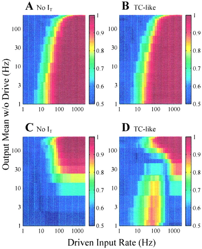
Summary of ROC area calculations performed for various combinations of spontaneous EPSP rate (spontaneous input rate;y-axis) and rate of excitatory or inhibitory drive (driven input rate; x-axis). ROC area plots summarize ∼800 combinations of spontaneous input rate and driven input rate, each leading to a number between 0.5 (chance level) and 1 (perfectly detectable). A, ROC area when the low-threshold Ca²⁺ current, I_T, is not included in the simulations (g_T = 0.2 mS/cm²). B,I_T is included in the model in a TC-like manner (g_T = 0.2 mS/cm²; V_h = −70 mV; V_L = −65 mV). C,I_T is included in the model in a TRN-like manner (g_T = 0.2 mS/cm²; V_h = −60 mV; V_L = −65 mV). D–F, Same as A–C, except the drive is inhibitory.

Figure 3A shows that for spontaneous input rates below ∼100 EPSPs/sec, a relatively constant amount of excitatory drive leads to detectable signal (for a ROC area of 0.8, ∼15 EPSPs/sec drive is required). However, when the spontaneous input rate increases to >100 EPSPs/sec, the amount of excitatory drive necessary to maintain detectability increases. This leads to a sloped (nonvertical) interface between low and high ROC area for a ρ_S of >100 EPSPs/sec. Despite this changing threshold of detectability, ROC area is always a monotonic increasing function of the rate of excitatory drive (left to right). Thus, elevated spontaneous input can suppress the detectability of excitatory inputs, but increasing excitatory drive never decreases detectability (Fig. 3A).

Figure 3, A and D, shows that excitatory and inhibitory drivers are not equivalent with respect to postsynaptic detectability. In the inhibitory case, spontaneous activity in the postsynaptic neuron is required so that inhibitory drive may be detected as a suppressed spike count (i.e., detectability is near zero for a ρ_S of <100 EPSPs/sec). To clarify this point, Figure 4, A andC, shows the ROC analysis of Figure 3, A andD, replotted with the mean output rate of the postsynaptic neuron in the absence of drive on the y-axis (no change to the x-axis, which still represents the rate of excitatory or inhibitory drive). This transformation of the y-axis is possible because in the absence of drive, the mean firing rate of the postsynaptic neuron is a monotonic increasing function of the rate of spontaneous EPSPs (recall Fig. 1B). Figure4B shows that for a ROC area of 0.8, spontaneous activity of ∼30 EPSPs/sec is needed. However, there is no such requirement in the case of excitatory drive (Fig.4A).

Fig. 4.

ROC analysis from Figure 3, A,B, D, and E replotted as a function of mean output rate of the postsynaptic neuron in the absence of drive (y-axis) and rate of excitatory or inhibitory drive (x-axis). This transformation is possible because in the absence of drive, the mean firing rate of the postsynaptic neuron is a monotonic increasing function of the spontaneous EPSP rate.

ROC calculations with a TC-like, low-threshold calcium current

To quantify the detectability of excitatory versus inhibitory drive in a TC neuron model that includes the low-threshold Ca²⁺ current,I_T, the parameterg_T in the IFB model was changed to the standard value of 0.2 mS/cm² (Table 1). Here V_h, the threshold for activation/inactivation of I_T, is −70 mV, 5 mV less than the resting membrane potential,V_L = −65 mV. Thus,I_T is TC-like (i.e., inactivated at rest), and the IFB model responds with bursts only after release from hyperpolarization.

Figure 3, B and E, summarizes ROC analysis for the TC-like IFB model under the influence of spontaneous EPSPs and either excitatory (Fig. 3B) or inhibitory (Fig.3E) drive. Figure 3B is nearly identical to Figure 3A, so the presence ofI_T has little effect on the detectability of excitatory drive, because all inputs to the IFB model are depolarizing and, consequently,I_T remains inactivated. However, Figure 3, D and E, shows thatI_T has a significant effect on the detectability of inhibitory drive. In this case, clusters of IPSPs from the inhibitory drive occasionally deinactivateI_T. If additional inhibition does not occur, then the membrane potential relaxes towardV_L until the burst thresholdV_h is crossed, thereby activatingI_T. Often an appropriately timed spontaneous EPSP accelerates this process. The elevated ROC area observed in Figure 3E (ρ_S < 160 EPSPs/sec and two IPSPs/sec < ρ_D < 100 IPSPs/sec) is attributable to bursts that lead to an elevated spike count distinguishable from that observed in the absence of inhibitory drive; other regions of high ROC area in Figure 3, D andE, reflect a reduced spike count. Figure4D also shows that in the presence ofI_T, spontaneous activity is not required for inhibitory drive to be detectable. Notice that the location of elevated ROC area implies that detectability is no longer a monotonic increasing function of the rate of inhibitory drive; that is, if the inhibitory drive is sufficiently strong, the relief from inhibition required for bursts does not occur.

To clarify this, Figure 5 shows three representative plots of the IFB model membrane potential for a spontaneous (excitatory) input rate of ρ_S = 30 EPSPs/sec (Fig. 5A). Consistent with Figure1B, this rate of spontaneous input leads to almost no response (Fig. 5D, gray line) (less than one trial in a thousand results in a spike). However, when this spontaneous input is supplemented with an excitatory drive rate of ρ_D = 30 EPSPs/sec in Figure 5B, tonic spikes are observed, and the histogram shifts rightward (28.4 ± 10.8 spikes/sec) (Fig. 5D, black line).

Fig. 5.

A, Representative membrane potential time courses (200 msec in duration) for the IFB model with TC-like, low-threshold Ca²⁺ current receiving spontaneous EPSPs at 30 EPSPs/sec (no response). B, Time courses when 30 EPSPs/sec of spontaneous input is augmented by 30 IPSPs/sec of excitatory drive. C, Cell response increases when 30 EPSPs/sec of spontaneous input is combined with 30 IPSPs/sec of inhibitory drive. D, E, Histograms of spike counts for 1000 trials and the corresponding ROC area calculations. Pr, Probability.

In Figure 5C, inhibitory drive is included at a rate of ρ_D = 30 IPSPs/sec, resulting in numerous IPSPs. Interestingly, although the driving input is inhibitory, the histogram of spike counts again shifts rightward (29.1 ± 14.7 spikes/sec). Focusing on the ROC area in the case of inhibitory drive, we see that postinhibitory rebound bursting mediated byI_T causes the inhibitory drive to be nearly perfectly detectable (0.99 in Fig. 5E), despite the fact that the spontaneous activity of the neuron is negligible in the absence of drive (Fig. 5A).

When the IFB model neuron was augmented to include the hyperpolarization-activated cation current,I_sag, ROC area calculations were qualitatively similar to those performed in the absence of this low-threshold current for both excitatory and inhibitory drive (data not shown; results are similar to Fig.3B,E). Interestingly,I_sag does enlarge the region over which the presence of I_T allows the detection of inhibitory drive (Fig.6).

Fig. 6.

ROC analysis for the IFB model in the presence (○) and absence (●) of the hyperpolarization-activated cation current, I_sag, as a function of the rate of inhibitory drive (x-axis) for a spontaneous excitatory input rate of 10 EPSPs/sec. In the absence ofI_sag, this corresponds to a cross section of Figure 3E.

ROC calculations with a TRN-like, low-threshold calcium current

In TC cells at rest, I_T is inactivated, i.e., the resting membrane potential is greater than the threshold for activation/inactivation of the low-threshold Ca²⁺ current (V_L >V_h). However, in TRN neurons, the threshold for activation of I_T is more depolarized than that in TC cells (Huguenard and Prince, 1992). Thus, we set the parameter V_h to −60 mV (5 mV greater than the resting membrane potential,V_L = −65 mV) so that the IFB model is TRN-like (V_h >V_L) and responds to sufficiently intense depolarization with a low-threshold Ca²⁺ spike.

Figure 3, C and F, summarizes ROC analysis for the TRN-like IFB model when the drive is either excitatory (Fig.3C) or inhibitory (Fig. 3F). Although the overall comparison of C and F with Band E in Figure 3 gives the impression that the effects of TRN-like I_T are subtle, there are some differences. For example, the distinction between Figure 3,C and A, is certainly greater than that between Figure 3, B and A, demonstrating that the presence of I_T influences the detectability of excitatory drive in the TRN-like IFB model (as opposed to the TC-like case, in which it had no effect). Interestingly, the presence of TRN-like I_T has an overall effect of decreasing the region of elevated ROC area. In particular, the threshold for detectability of excitatory inputs increased when the spontaneous input rate was 10–100 EPSPs/sec (see notch in Fig. 3,C compared with A).

The ROC areas in the presence of TRN-likeI_T and inhibitory drive (Fig.3F) are distinct from both the TC-like case (Fig.3E) and the result in the absence ofI_T (Fig. 3D). There is an island of detectability for spontaneous input rates between 30 and 300 EPSPs/sec. At ρ_S = 100 EPSPs/sec, for example, ROC area first increases, then decreases, and then increases again as a function of the rate of inhibitory drive (ρ_S). The elevated detectability for spontaneous input rates between 30 and 300 EPSPs/sec is analogous to the region of elevated ROC area in the TC-like case. Here, the excitatory spontaneous input depolarizes the model membrane potential enough so that certain levels of inhibitory drive lead to postinhibitory rebound bursts. This is demonstrated in Figure 7C using ρ_S = 100 EPSPs/sec and ρ_D = 30 IPSPs/sec. The TRN-like IFB model shows increased spike count for excitatory drive (Fig. 7B), but for these values of ρ_S and ρ_D, the detectability of inhibitory drive (0.94) (Fig. 7E) is greater than that of excitatory drive (0.82) (Fig. 7D).

Fig. 7.

A, Representative membrane potential time courses for the IFB model with TRN-like, low-threshold Ca²⁺ current receiving spontaneous EPSPs at 100 EPSPs/sec. B, Time courses when 30 EPSPs/sec of excitatory drive is included. C, Cell response increases when 30 IPSPs/sec of inhibitory drive is included. D,E, Histograms of spike counts for 1000 trials and the corresponding ROC area calculations. Pr, Probability.

Figure 3F shows moderate ROC area (0.7–0.8) extending to lower levels of spontaneous EPSP rates than in the absence ofI_T (compare Fig. 3D), although the effect is not as strong as whenI_T is TC-like (compare Fig.3E) and occurs over a different range of rates of inhibitory drive (Fig. 3F, ρ_D of >100 IPSPs/sec; Fig. 3E, ρ_D of <100 IPSPs/sec). This region of moderate ROC area is attributable to detectable suppression of bursts that are induced by spontaneous excitatory input in the absence of inhibitory drive (data not shown).

Voltage dependence of ROC calculations

In the above simulations, ROC area analysis has been performed using the IFB model both with and withoutI_T. In the presence ofI_T, we have found that the detectability of inhibitory inputs was dependent on the relationship between the IFB model resting membrane potential,V_L, and the threshold (V_h) for activation/inactivation ofI_T. In particular, a region of elevated detectability of inhibitory inputs that is prominent when the IFB model is TC-like and I_T is inactivated at rest (V_L >V_h) (Fig. 3E) is reduced or absent when the IFB model is TRN-like andI_T is deinactivated at rest (V_L <V_h) (Fig. 3F). However, because modulatory inputs can change the resting membrane potential of both TC and TRN neurons, it is important to clarify how the detectability of inhibitory input may depend on the resting membrane potential.

To address this question for inhibitory inputs, Figure8A–E presents ROC area calculations in which V_L was varied from −75 through −55 mV (Table 1). In these calculations,V_h = −70 mV, and Figure 8Cthus reproduces Figure 3E. Figure 8, D andE, shows that changing V_Lto more depolarized values (−60 or −55 mV) has little effect on the ROC area calculation. That is, Figure 8C–E shows a region of elevated detectability for inhibitory inputs induced byI_T. Conversely, Figure 8, Aand B, shows that changing the resting membrane potential to more hyperpolarized values (V_L = −75 or −70 mV) reduces the detectability of inhibitory inputs. Interestingly, the result in Figure 8A (whereV_L = −75 andV_h = −70 mV) is very similar to the ROC analysis of the TRN-like IFB model shown in Figure 3F(where V_L = −65 andV_h = −60 mV), indicating the importance of the relationship betweenV_L andV_h in determining whether the model bursts in response to depolarization or relief from hyperpolarization and the consequent detectability (or lack thereof) of inhibitory input. Indeed, the overall structure of Figure 8A–J (whereV_h = −60 mV so that Fig.8H thus corresponds to the TRN-like result of Fig.3F) suggests that the important features of the ROC analysis plots are determined by the quantityV_L −V_h.

Fig. 8.

ROC area calculations resulting from inhibitory drive, where V_L is varied from −75 to −55 mV. A–E, V_h = −70 mV so that C is a reproduction of the TC-like result of Figure 3E, where the resting membrane potential is given by the standard value of V_L = −65 mV.F–J, V_h = −60 mV so that H is a reproduction of the TRN-like result of Figure 3F.

Calculations similar to those presented in Figure 8 indicate that the resting membrane potential affects the detectability of excitatory input as well (data not shown). However, the similarity of TC-like and TRN-like responses to excitatory inputs (Fig. 3, compare Bwith C) means that the variation in the ROC analysis is modest compared with that observed in Figure 8.

ROC area analysis using a Hodgkin–Huxley-like, conductance-based model

To determine the degree to which the above results generalize, we performed ROC analysis using a truncation of the McCormick–Huguenard TC neuron model (Huguenard and McCormick, 1992, 1994; McCormick and Huguenard, 1992; Mukherjee and Kaplan, 1995). The current balance equation included five currents: fast Na⁺and K⁺ (delayed rectifier) currents responsible for action potential generation,I_Na andI_K-DR; K⁺and Na⁺ leak currents,I_Kleak andI_Naleak; the low-threshold Ca²⁺ current,I_T; and in some cases,I_sag (for details, seehttp://www.as.wm.edu/Faculty/Smith.html). Action potentials were counted according to the number of times the membrane potential was depolarized above an arbitrary threshold value of −30 mV. We found the ROC area analysis of the Hodgkin–Huxley (HH) and IFB models to be in quantitative agreement, regardless of whether the drive was excitatory or inhibitory. This agreement is attributable in part to the similarity of the input–output relationships of the HH and IFB models (data not shown) when both are constrained to fit experimental observations of TC neuron responses from cat thalamic slices (Smith et al., 2001).

ROC calculations with balanced excitatory and inhibitory spontaneous input

In the simulations presented thus far, the detectability of excitatory or inhibitory drive has been quantified assuming that the background activity of the IFB model is caused solely by excitatory spontaneous input. However, it is more realistic to presume that the background activity of the output neuron in Figure 1Ais caused by a mixture of excitatory and inhibitory spontaneous input. To represent this possibility, the current balance equation for the IFB model was extended to include two spontaneous synaptic current terms, one excitatory and the other inhibitory. When the spontaneous excitatory and inhibitory inputs are balanced (both arriving at identical ρ_S rates), the input–output relationship for the IFB model in the absence of drive is significantly shallower than the result for purely excitatory spontaneous input (data not shown).

Despite this difference, the ROC analysis for balanced excitatory and inhibitory spontaneous input is qualitatively similar to the results for pure excitatory spontaneous input (data not shown, similar to Fig.3). However, in both the absence and the presence ofI_T, the combination of excitatory and inhibitory spontaneous input does slightly improve detectability of excitatory input when the spontaneous input rate is high (ρ_S of >100 PSPs/sec). When the driving input is inhibitory, the combination of excitatory and inhibitory spontaneous input tends to decrease detectability at high spontaneous input rates but does not eliminate the region of elevated ROC area observed in the presence of I_T (compare Fig.3E). When the parameters forI_T are TRN-like, a corresponding trend is observed; mixed excitatory and inhibitory spontaneous input leads to a slight increase in detectability when the drive is excitatory and a slight decrease in detectability when the drive is inhibitory, but only when the spontaneous input rate is high.

DISCUSSION

Using an integrate-and-fire-or-burst TC neuron model and a more detailed Hodgkin–Huxley-style model (data not shown), we have quantified the detectability of stochastic excitatory and inhibitory drive in the presence and absence of the low-threshold Ca²⁺ current,I_T. By calculating ROC area, we quantified detectability when the model neuron received postsynaptic potentials from an excitatory source that evokes spontaneous activity (i.e., noise) and a second (excitatory or inhibitory) source that represents an afferent signal (Fig. 1A). Similar results were obtained when the model neuron received spontaneous postsynaptic potentials from a combination of excitatory and inhibitory sources (data not shown).

We find that in the absence of I_Tdetectability is typically poorer for inhibitory than for excitatory drive. This is particularly true for low to moderate levels of spontaneous activity in the postsynaptic neuron, because spontaneous activity is required for inhibitory drive to be detected as a suppressed spike count. In the presence ofI_T, results depend strongly on whether the threshold for I_T activation lies above the resting membrane potential (TRN-like) or below it (TC-like). In the latter case, I_T enables the detection of inhibitory drivers even when the postsynaptic neuron is not spontaneously active.

The qualitative aspects of the ROC area analysis presented here are not sensitive to the size of the spontaneous and driven postsynaptic potentials (A_S andA_D), although a threefold change does shift areas of elevated detectability toward higher or lower EPSP/IPSP rates (data not shown). Interestingly, we found that changes in resting membrane potential can significantly change the overall dependence of the detectability of inhibitory input on spontaneous and driven input rates (Fig. 8). This suggests that the detection of inhibitory inputs enabled by I_T may be sensitive to neuromodulation that affects the resting membrane potential of TC neurons.

Limitations of single-compartment modeling

Because both of the models used (IFB and Hodgkin–Huxley) are single-compartmental models, a limitation of this work is that some results may not generalize to situations involving temporally or spatially patterned synaptic input distributed over dendritic arbors. Although excitatory and inhibitory inputs are demonstrably not equivalent in isopotential compartmental models, one might devise a multicompartmental model with various assumptions about dendritic architecture, the distribution of ionic currents, and the spatial organization of synaptic inputs, for which excitatory and inhibitory inputs are less distinguishable on the basis of detectability. Nevertheless, the use of single-compartmental models is appropriate on several grounds. As a practical matter, the choice is motivated by a desire to perform adequate statistics of the stochastic responses that we quantify. Furthermore, previous cable modeling of current flow within dendritic arbors of thalamic relay cells has concluded that they are electronically compact. Thus, a postsynaptic potential generated anywhere in the dendritic arbor of a relay cell spreads with relatively little attenuation throughout the arbor and to its soma (Bloomfield and Sherman, 1989). Finally, the experimental evidence that would allow one to associate various compartments of a multicompartmental model with specific synaptic inputs suggests that excitatory and inhibitory inputs are largely overlapping (Wilson et al., 1984). In the absence of spatial heterogeneity of excitatory and inhibitory inputs, we expect the results of multicompartmental modeling to largely agree with the single compartment modeling results presented here.

Can inhibitory inputs be drivers to thalamus?

It has been stressed previously (Sherman and Guillery, 1998, 2001) that afferent inputs to thalamic relay cells can be divided into at least two functionally distinct groups: drivers and modulators. Drivers of thalamic relay cells transmit the basic information to be relayed to the cortex, act through ionotropic receptors that have a fast postsynaptic effect, and, where practical, have been identified as the transmitter of receptive field properties. Modulators, on the other hand, may activate metabotropic receptors having a slow and prolonged postsynaptic effect, and these afferents produce only subtle changes in receptive field properties. The retinal input to the lateral geniculate nucleus, the inferior collicular input to the medial geniculate nucleus, and the medial lemniscal input to the ventrobasal complex are examples of drivers, and so are cortical layer 5 inputs to many higher-order thalamic relays. Although drivers can be clearly recognized for some other thalamic relays, the identity of the drivers is not yet obvious in some nuclei (Sherman and Guillery, 1998, 2001). Examples of modulators include local GABAergic inputs, corticothalamic feedback from layer 6 and cholinergic, noradrenergic, and serotonergic inputs from brainstem. It is possible to view the spontaneous (noise) input leading to background activity in the IFB model as a modulator, because the time constant for spontaneous EPSPs can be slowed considerably without qualitative changes to the detectability analysis (data not shown).

A number of criteria to distinguish drivers from modulators for thalamic relays have been suggested; for example, cross-correlograms from driver inputs are likely to be sharply peaked compared with those from modulatory inputs. Certainly an important functional criteria for a driver input is an ability to transfer information efficiently across the synapse to the relay cell, and thus, the presence or absence of driving input must be detectable on the basis of the postsynaptic neuron response. In the absence of knowledge about presynaptic firing rates, our simulations show that overall detectability is poorer for inhibitory drive than excitatory drive. Thus, we suggest adding to the list of criteria to distinguish drivers from modulators the proposition that, other things being equal, inhibitory inputs are less likely to be drivers than excitatory inputs.

However, an important caveat to this conclusion is that over a certain range of spontaneous and driven activity, the low-threshold Ca²⁺ current,I_T, may allow the detection of inhibitory drive. Indeed, the calculations of elevated detectability mediated by I_T presented above suggest three criteria for the identification of an inhibitory driver that usesI_T: (1) a candidate inhibitory driver must provide IPSPs at a rate that results in postinhibitory rebound bursting and elevated spike count in the postsynaptic neuron (in Fig.3E, this range is 10–100 IPSPs/sec), (2) the spontaneous activity of the postsynaptic neuron must be modest (<30 spikes/sec in Fig. 4D), and (3) for robust detectability, the postsynaptic neuron must express the low-threshold Ca²⁺ current in a TC-like manner, so that inhibitory drive can deinactivate I_T. In light of these results, we suggest that inhibitory projections to thalamic relay nuclei should not be presumed to be drivers unless the spontaneous activity of the postsynaptic neuron is relatively high or there is reason to believe that these three conditions forI_T-mediated detectability hold. Because relay cells responding in burst mode have nonlinear input–output relationships, we also suggest thatI_T-mediated detection of inhibitory drive is unlikely to be a mechanism associated with faithful relay of information to the cortex (Sherman, 2001).

The implications of these criteria for inhibitory drivers are potentially far reaching. For example, textbook accounts (Purves et al., 1997; Kandel et al., 2000) imply that the basal ganglia relays information to the neocortex via a GABAergic inhibitory input to ventral anterior and lateral nuclei of the thalamus. Because available evidence suggests that the responses of relay cells of these nuclei are primarily in tonic mode (Zirh et al., 1998; Radhakrishnan et al., 1999;Magnin et al., 2000), it is unlikely that these nuclei detect inhibitory input via an I_T-dependent mechanism. Thus, using the criteria for inhibitory drivers listed above, one might suggest that these nuclei detect inhibition through the suppression of spontaneous and relatively high-frequency tonic responses. Alternatively, the basal ganglia input to the ventral anterior and lateral nuclei of the thalamus might not be functioning as an inhibitory driver but rather as an inhibitory modulator of another input or inputs to these thalamic nuclei, for example, input from the cerebellum (Mason et al., 2000; Sakai et al., 2000) and/or layer 5 of the motor cortex (cf. Guillery and Sherman, 2002).

To give another example, the identification of inhibitory Purkinje cells of the cerebellar cortex as drivers of the deep cerebellar nuclei may or may not be consistent with the criteria for inhibitory drivers discussed above. If not, another candidate driver input to the deep cerebellar nuclei is excitation from mossy or climbing fiber axon branches, in which case Purkinje cell activity would be an inhibitory modulator rather than an inhibitory driver, providing the basic information for the deep cerebellar nuclei to transmit to other brain centers. Rethinking of the functional organization of this and other neural pathways may be required if responses of presumed inhibitory drivers and their postsynaptic targets are not consistent with the criteria for inhibitory drivers proposed above.

REFERENCES

- 1.Bloomfield SA, Sherman SM. Dendritic current flow in relay cells and interneurons of the cat's lateral geniculate nucleus. Proc Natl Acad Sci USA. 1989;86:3911–3914. doi: 10.1073/pnas.86.10.3911. [DOI] [PMC free article] [PubMed] [Google Scholar]
- 2.Destexhe A, Mainen Z, Sejnowski T. Synthesis of models for excitable membranes, synaptic transmission and neuromodulation using a common kinetic formalism. J Comput Neurosci. 1994;1:195–230. doi: 10.1007/BF00961734. [DOI] [PubMed] [Google Scholar]
- 3.Dossi RC, Nunez A, Steriade M. Electrophysiology of a slow (0.5–4 Hz) intrinsic oscillation of cat thalamocortical neurones in vivo. J Physiol (Lond) 1992;447:215–234. doi: 10.1113/jphysiol.1992.sp018999. [DOI] [PMC free article] [PubMed] [Google Scholar]
- 4.Gabbiani F, Koch C. Signal processing techniques for spike train analysis using MatLab. In: Koch C, Segev I, editors. Methods in neuronal modeling: from ions to networks, Ed 2. MIT; Cambridge, MA: 1998. [Google Scholar]
- 5.Green D, Swets J. Signal detection theory and psychophysics. Wiley; New York: 1966. [Google Scholar]
- 6.Guido W, Lu S-M, Vaughan J, Godwin D, Sherman SM. Receiver operating characteristic (ROC) analysis of neurons in the cat's lateral geniculate nucleus during tonic and burst response mode. Vis Neurosci. 1995;12:723–741. doi: 10.1017/s0952523800008993. [DOI] [PubMed] [Google Scholar]
- 7.Guillery RW, Sherman SM. Thalamic relay functions and their role in corticocortical communication: generalizations from the visual system. Neuron. 2002;33:1–20. doi: 10.1016/s0896-6273(01)00582-7. [DOI] [PubMed] [Google Scholar]
- 8.Huguenard JR, McCormick D. Simulation of the currents involved in rhythmic oscillations in thalamic relay neurons. J Neurophysiol. 1992;68:1373–1383. doi: 10.1152/jn.1992.68.4.1373. [DOI] [PubMed] [Google Scholar]
- 9.Huguenard J, McCormick D. Electrophysiology of the neuron. Oxford UP; New York: 1994. [Google Scholar]
- 10.Huguenard JR, Prince DA. A novel T-type current underlies prolonged Ca2+-dependent burst firing in GABAergic neurons of rat thalamic reticular nucleus. J Neurosci. 1992;12:3804–3817. doi: 10.1523/JNEUROSCI.12-10-03804.1992. [DOI] [PMC free article] [PubMed] [Google Scholar]
- 11.Jahnsen H, Llinas R. Electrophysiological properties of guinea-pig thalamic neurones: an in vitro study. J Physiol (Lond) 1984a;349:205–226. doi: 10.1113/jphysiol.1984.sp015153. [DOI] [PMC free article] [PubMed] [Google Scholar]
- 12.Jahnsen H, Llinas R. Ionic basis for the electroresponsiveness and oscillatory properties of guinea-pig thalamic neurones in vitro. J Physiol (Lond) 1984b;349:227–247. doi: 10.1113/jphysiol.1984.sp015154. [DOI] [PMC free article] [PubMed] [Google Scholar]
- 13.Kandel ER, Schwartz JH, Jessell TM. Principles of neural science. McGraw Hill; New York: 2000. [Google Scholar]
- 14.Keener J, Hoppensteadt F, Rinzel J. Integrate-and-fire models of nerve membrane response to oscillatory input. SIAM J Appl Math. 1981;41:503–517. [Google Scholar]
- 15.MacMillan N, Creelman C. Detection theory: a user's guide. Cambridge UP; Cambridge, MA: 1991. [Google Scholar]
- 16.Magnin M, Morel A, Jeanmonod D. Single-unit analysis of the pallidum, thalamus and subthalamic nucleus in Parkinsonian patients. Neuroscience. 2000;96:549–564. doi: 10.1016/s0306-4522(99)00583-7. [DOI] [PubMed] [Google Scholar]
- 17.Mason A, Ilinsky IA, Maldonado S, Kultas-Ilinsky K. Thalamic terminal fields of individual axons from the ventral part of the dentate nucleus of the cerebellum in Macaca mulatta. J Comp Neurol. 2000;421:412–428. [PubMed] [Google Scholar]
- 18.McCormick D, Huguenard J. A model of the electrophysiological properties of thalamocortical relay neurons. J Neurophysiol. 1992;68:1384–1400. doi: 10.1152/jn.1992.68.4.1384. [DOI] [PubMed] [Google Scholar]
- 19.Mukherjee P, Kaplan E. Dynamics of neurons in the cat lateral geniculate nucleus: in vivo electrophysiology and computational modeling. J Neurophysiol. 1995;74:1222–1243. doi: 10.1152/jn.1995.74.3.1222. [DOI] [PubMed] [Google Scholar]
- 20.Purves D, Augustine GJ, Fitzpatrick D, Katz LC, Lamantia A-S, McNamara JO. Neuroscience. Sinauer; Sunderland, MA: 1997. [Google Scholar]
- 21.Radhakrishnan V, Tsoukatos J, Davis KD, Tasker RR, Lozano AM, Dostrovsky JO. A comparison of the burst activity of lateral thalamic neurons in chronic pain and non-pain patients. Pain. 1999;80:567–575. doi: 10.1016/S0304-3959(98)00248-6. [DOI] [PubMed] [Google Scholar]
- 22.Rall W. Distinguishing theoretical synaptic potentials computed for different soma-dendritic distributions of synaptic inputs. J Neurophysiol. 1967;30:1138–1168. doi: 10.1152/jn.1967.30.5.1138. [DOI] [PubMed] [Google Scholar]
- 23.Rinzel J. Models in neurobiology. In: Enns RH, Jones BL, Miura RM, Rangnekar SS, editors. Nonlinear phenomena in physics and biology, Vol 75. North Atlantic Treaty Association Advanced Study Institute; Alberta, Canada: 1980. pp. 347–367. [Google Scholar]
- 24.Sakai ST, Stepniewska I, Qi HX, Kaas JH. Pallidal and cerebellar afferents to pre-supplementary motor area thalamocortical neurons in the owl monkey: a multiple labeling study. J Comp Neurol. 2000;417:164–180. [PubMed] [Google Scholar]
- 25.Sherman SM. Tonic and burst firing: dual modes of thalamocortical relay. Trends Neurosci. 2001;24:122–126. doi: 10.1016/s0166-2236(00)01714-8. [DOI] [PubMed] [Google Scholar]
- 26.Sherman SM, Guillery RW. The functional organization of thalamocortical relays. J Neurophysiol. 1996;76:1367–1395. doi: 10.1152/jn.1996.76.3.1367. [DOI] [PubMed] [Google Scholar]
- 27.Sherman SM, Guillery RW. On the actions that one nerve cell can have on another: distinguishing “drivers” from “modulators”. Proc Natl Acad Sci USA. 1998;95:7121–7126. doi: 10.1073/pnas.95.12.7121. [DOI] [PMC free article] [PubMed] [Google Scholar]
- 28.Sherman SM, Guillery RW. Exploring the thalamus. Academic; San Diego: 2001. [Google Scholar]
- 29.Sherman SM, Koch C. Thalamus. In: Shepherd G, editor. Synaptic organization of the brain, Ed 4. Oxford UP; New York: 1998. pp. 246–278. [Google Scholar]
- 30.Smith G, Sherman SM. Detectability of excitatory versus inhibitory drive in a stochastic thalamocortical relay neuron model. Soc Neurosci Abstr. 2001;27:723.21. doi: 10.1523/JNEUROSCI.22-23-10242.2002. [DOI] [PMC free article] [PubMed] [Google Scholar]
- 31.Smith G, Cox C, Sherman SM, Rinzel J. Fourier analysis of sinusoidally-driven thalamocortical relay neurons and a minimal intergrate-and-fire-or-burst model. J Neurophysiol. 2000;83:588–610. doi: 10.1152/jn.2000.83.1.588. [DOI] [PubMed] [Google Scholar]
- 32.Smith G, Cox C, Sherman SM, Rinzel J. Spike-frequency adaptation in sinusoidally-driven thalamocortical relay neurons. Thalamus and Related Systems. 2001;1:135–156. [Google Scholar]
- 33.Tuckwell H. Introduction to theoretical neurobiology: nonlinear and stochastic theories, Vol 2. Cambridge UP; Cambridge, UK: 1988. [Google Scholar]
- 34.Tuckwell H. Stochastic processes in the neurosciences. Society for Industrial and Applied Mathematics; Philadelphia: 1989. [Google Scholar]
- 35.Wang XJ. Multiple dynamical modes of thalamic relay neurons: rhythmic bursting and intermittent phase-locking. Neuroscience. 1994;59:21–31. doi: 10.1016/0306-4522(94)90095-7. [DOI] [PubMed] [Google Scholar]
- 36.Wilson JR, Friedlander MJ, Sherman SM. Fine structural morphology of identified X- and Y-cells in the cat's lateral geniculate nucleus. Proc R Soc Lond B Biol Sci. 1984;221:411–436. doi: 10.1098/rspb.1984.0042. [DOI] [PubMed] [Google Scholar]
- 37.Zirh TA, Lenz FA, Reich SG, Dougherty PM. Patterns of bursting occurring in thalamic cells during parkinsonian tremor. Neuroscience. 1998;83:107–121. doi: 10.1016/s0306-4522(97)00295-9. [DOI] [PubMed] [Google Scholar]