Frealign: An exploratory tool for single particle cryo-EM

Abstract

Frealign is a software tool designed to process electron microscope images of single molecules and complexes to obtain reconstructions at the highest possible resolution. It provides a number of refinement parameters and options that allow users to tune their refinement to achieve specific goals, such as masking to classify selected regions within a particle, control over the refinement of specific alignment parameters to accommodate various data collection schemes, refinement of pseudo-symmetric particles, and generation of initial maps. This chapter provides a general overview of Frealign functions and a more detailed guide to using Frealign in typical scenarios.

1. Introduction and philosophy

Frealign (Grigorieff, 1998, 2007) is an image processing tool that can be used to calculate and refine three-dimensional (3D) structures of macromolecular assemblies that are calculated from images collected on an electron microscope. Its development began in 1996 at the MRC Laboratory of Molecular Biology (Cambridge, UK) with the aim to implement a fast and accurate projection matching algorithm, and to calculate 3D reconstructions that are fully corrected for the contrast transfer function (CTF) of the microscope. Besides the author, a number of other people have contributed to the development of Frealign in various ways, including Tim Grant, Richard Henderson, Dmitry Lyumkis, Alexis Rohou, Charles Sindelar, Alex Stewart, Douglas Theobald, Christine Villeneuve and Matthias Wolf (Lyumkis et al., 2013; Sindelar and Grigorieff, 2012; Stewart and Grigorieff, 2004; Wolf et al., 2006), and a GPU-accelerated version was developed by Yifan Cheng and his group (Li et al., 2010). Its primary application has remained the refinement of particle alignments and 3D reconstruction optimized to reveal details at the highest possible resolution. Other features were added over the years, including refinement of microscope defocus and magnification, correction for the Ewald sphere curvature (Wolf et al., 2006), processing of helical particles (Alushin et al., 2010), 3D classification (Lyumkis et al., 2013) and density masking. Furthermore, algorithms and run scripts were developed to take advantage of parallel computing environments to speed up processing. These developments have made Frealign one of the fastest, most versatile image processing tools for the refinement of single particle structures, yielding some of the best resolved reconstructions to date.

Frealign is freely available for download from the Grigorieff lab web page (http://grigoriefflab.janelia.org/frealign). Its primary purpose is to serve as a platform for the development of new image processing algorithms and to support projects in the Grigorieff lab and at the MRC-LMB. Little attention has therefore been devoted to user friendliness and documentation, which require time and resources that were instead devoted to support the primary mission of Frealign. However, some help is provided by the Frealign user forum on the Grigorieff lab web page, which allows users to ask questions and read up on previously answered questions.

The more narrowly defined scope and purpose of Frealign distinguish it from software packages that are designed to offer a complete set of tools for single particle image processing, including movie processing, CTF determination and correction, particle selection, initial map generation, 2D and 3D classification, refinement and reconstruction. Using Frealign requires the use of other software to carry out many of the steps necessary to arrive at a 3D reconstruction. Tools for some of these steps have also been developed as stand-alone applications in the Grigorieff lab, such as Signature (Chen and Grigorieff, 2007), CTFFIND (Mindell and Grigorieff, 2003; Rohou and Grigorieff, 2015), Unblur/Summovie (Grant and Grigorieff, 2015b) and magnification distortion correction (Grant and Grigorieff, 2015a), which are also freely available to users. Some of these stand-alone applications will briefly be described at the end of this chapter. However, the main emphasis of the chapter will be on the use of Frealign, describing typical application scenarios and providing practical advice on how to achieve the highest possible resolution. This differs from an earlier paper on Frealign (Grigorieff, 2007) that focused more on algorithmic features.

2. Frealign elements at a glance

2.1. Running Frealign

The Frealign distribution is available from the Grigorieff lab web page (http://grigoriefflab.janelia.org/frealign) and contains compiled versions of the programs for 64-bit Linux and Mac OS systems. Installation requires unpacking of the archive and adding the path to the compiled programs and run scripts to the user environment.

Frealign has been developed to run on Linux and Max OS workstations and is run from a command line inside a terminal. Many of the available commands can be listed by issuing the frealign_help command. These include frealign_run_refine and frealign_calc_reconstructions, commands that will start the refinement of a structure or calculate a 3D reconstruction using parameters from a previous Frealign run. The progress towards completion of a task can be followed by monitoring the file frealign.log. Apart from these high-level tasks (run scripts) there are also more primitive commands that call up one of the compiled programs that are part of the Frealign distributions, for example bfactor.exe, which allows users to apply a low-pass filter and sharpen a 3D reconstruction using a specified B-factor (see below).

Structure refinement in Frealign is performed iteratively. Each iteration takes input files from the previous cycle and produces new output files that can serve as input for a new cycle. The user can specify the number of cycles to run and how many computing resources to dedicate to the job (see below).

2.2. Required input

Most data used by Frealign is stored either in text files or image files. While the most extensively used and tested image format is the MRC format (Crowther et al., 1996), images stored using the Spider (Frank et al., 1996) and IMAGIC (van Heel et al., 1996) formats are also supported. A schematic overview of required and optional input and output files is shown in Fig. 1, together with some of the functional features discussed below. To run Frealign, the user has to set up a text file called mparameters (Fig. 2) that specifies

Figure 1.

Schematic overview of Frealign functions, input and output data. Some of the Frealign commands mentioned in the text are shown in Courier font above the functions or files they relate to. Features and files that are optional and not always used are shown with dashed borders. Frealign is run by a number of shell scripts that prepare input and output data, manage parallel execution and perform iterations when more than one cycle is run.

Figure 2.

Template for the mparameters file containing all the control parameters required to run Frealign. Each keyword has an assigned value or string (text) and, in most cases, a comment line explaining how the parameter should be set. The control parameters are divided into different sections to help users customize the parameters according to their environment and project. Parameters listed in the expert section usually do not need to be changed until refinement and classification have converged. These parameters allow users to tune their refinement to improve resolution but they require some experience to be set correctly.

• the computing architecture, for example cluster type and number of CPUs to use,

• the main Frealign control parameters, including the number of refinement cycles to run,

• data-specific parameters, such as input parameters and microscope settings,

• optional parameters to tune refinement,

• masking parameters.

Each input line in mparameters is annotated to help users choose appropriate settings. Many of the settings involve flags that can be set to “T” (for “true”) or “F” (for “false”) to turn a feature on or off. Besides mparameters the user also has to supply a particle image stack and a particle parameter file - a text file providing some information about each image in the stack. The images in the stack should be uniformly scaled, i.e. the average background (solvent) density should be set to zero and its variance to a specified value. In practice, it is sufficient to set the average density of each particle image to zero and its variance to a specified value. This scaling procedure includes the particle density and will therefore be less accurate than a procedure that only considered the background in the calculation. However, in tests comparing results with particles scaled with one of these two procedures, no noticeable differences were observed.

The particle parameter file contains one line of text for each image in the stack. It is therefore important to make sure that the number of lines (excluding comment lines) in a parameter file matches the number of images in the stack. Each line of text normally contains the following information:

• Euler angles (in degrees) and x,y translations (in Å) describing the alignment of the particle,

• micrograph identifier, image magnification and defocus,

• a parameter describing the membership of the particle to a class (occupancy),

• relative log likelihood for the particle given the map and alignment parameters,

• standard deviation of the estimated background noise,

• particle score.

At the beginning of a new project, when alignment parameters are not known, the user can supply an abbreviated particle parameter file that will contain only four numbers per line:

• an integer to identify the micrograph the particle came from,

• two defocus values and an astigmatic angle (in degrees) needed to describe the microscope CTF. These values are written out by the program CTFFIND (Mindell and Grigorieff, 2003; Rohou and Grigorieff, 2015), for example.

Frealign will convert this file into a full parameter file by adding random Euler angles, setting the particle translations to zero and filling in the rest of the parameters with nominal values that can then be updated in later refinement cycles.

2.3. Optional input

In most cases, users will also supply a 3D reconstruction (or several reconstructions for multi-reference refinement and classification, see below) on input that was obtained either from a previous Frealign run or through other means. The 3D reconstruction is used by Frealign as a reference to refine the particle parameters (see below). If no 3D reconstruction is supplied, Frealign will calculate one from the input particle parameters. If these parameters are given in the abbreviated format, i.e. no Euler angles and x,y translations are available, Frealign will calculate a 3D reconstruction using randomly assigned angles after converting the abbreviated parameter file to a full parameter file, thus creating a random startup structure (see below).

Finally, a 3D mask file can be specified in mparameters that Frealign will use to mask the input 3D reconstruction, allowing the user to focus on specific regions of the molecule during refinement (see below).

2.4. Output

Each refinement cycle performed by Frealign will generate a new particle parameter file and 3D reconstruction (if multiple references are used, parameter files and reconstructions are generated for each). A scratch directory used by Frealign to hold temporary files also contains 3D reconstructions calculated from half the data each. These are used by Frealign to calculate a Fourier Shell Correlation (FSC) curve to estimate the resolution of the final 3D structure (Harauz and van Heel, 1986). These half reconstructions can be ignored in a typical Frealign run but are sometimes useful if users would like to perform their own resolution estimation, for example using ResMap (Kucukelbir et al., 2014). The FSC curve for each reconstruction can be found in a resolution table at the end of the particle parameter file belonging to the reconstruction, and plots can be generated using the command frealign_plot_fsc. The table also contains other information, for example an adjusted FSC curve called Part_FSC, which estimates the resolution of the reconstruction (usually at the threshold value of 0.143, (Rosenthal and Henderson, 2003)) after removing all solvent noise. This adjusted curve should therefore be taken as the curve shown in publications to support resolution claims. While resolution estimates for reconstructions after removing solvent noise are often obtained by applying tight masks, Frealign obtains this estimate by considering the volume occupied by the particle (Sindelar and Grigorieff, 2012). The volume is calculated from the molecular mass of the particle provided by the user in mparameters using a conversion factor of 810 Da/nm³ (Matthews, 1968). The volume is also used to calculate the spectral signal-to-noise ratio (SSNR) present inside the particle (called Rec_SSNR in the final resolution table). The particle SSNR is used to apply an optimal filter to the final reconstruction (Sindelar and Grigorieff, 2012) if FFILT is set in mparameters. In addition to the SSNR filter, it is recommended to apply a negative B-factor to the final reconstruction to sharpen the density, and a low-pass filter with a cosine-edged cutoff to set terms beyond the resolution limit to 0. Both operations can be accomplished with bfactor.exe (see below).

2.5. Naming conventions

Frealign uses the following naming scheme for alignment parameter files and 3D reconstructions: file names consist of a seed that should identify the particle (for example 70S for the 70S ribosome), followed by “_M_rN” where M and N are integers that signify the refinement cycle number and reference, respectively. Typically, when initializing a Frealign run, only one reference is used (see below) and the refinement starts with cycle 1. Therefore, M should be set to 0 and N to 1 (e.g. “70S_0_r1”). The parameter files are expected to have the extension “.par” while particle image stacks and 3D reconstructions have extensions that depend on the file format. MRC/CCP4 files have the ending “.mrc”, Spider “.spi” and IMAGIC “.hed” and “.img”.

3. Algorithms

A description of the algorithms employed by Frealign to refine alignment parameters and perform classification is given in (Grigorieff, 2007). Briefly, Frealign performs projection matching to determine more accurate alignment parameters. Projections are calculated using the reference map provided on input and alignment parameters for each particle are updated according to the projection that generates the highest correlation coefficient. The user has a choice to search for projections with parameters close to those previously found (local search) by setting MODE to 1 in mparameters, or to perform a global parameter search with randomly generated parameters (MODE set to 2 and ITMAX set to the desired number of trials, e.g. 100) or with parameters systematically chosen according to a search grid (MODE set to 3 and DANG set to the desired angular step in degrees, e.g. 10). If MODE is set to 3, the user can also set DANG to 0 to let Frealign calculate an appropriate angular step, based on the particle radius and refinement resolution limit (see below) set by the user. The correlation coefficient calculated by Frealign is weighted according to the SSNR present in the particle images. The average particle SSNR is contained in the final resolution table (Part_SSNR), together with the FSC curve and other statistics. It is important not to delete this table from the end of a parameter file because it is read by Frealign in the next refinement cycle.

3D classification is done using a maximum likelihood approach. Frealign calculates relative likelihoods (i.e. likelihood values that are missing constants necessary to put the likelihoods on an absolute scale) of each particle given a 3D reference map and a set of alignment parameters. The logarithms of these values are listed in the particle parameter files (column LogP). For classification, multiple reference structures are used and likelihood values are calculated for each. At the end of a refinement cycle, these likelihood values are converted by the program calc_occ.exe (part of the Frealign distribution and executed automatically by the run script) into weights, so-called occupancies (column OCC) that determine the partitioning of each particle into the different classes. To speed up classification and improve convergence, the user can specify if Frealign should refine alignment parameters with every classification cycle, or if alignment parameter refinement should only be done every N^th cycle. Typically, alignment parameter refinement should only be done every 3^rd or 4^th cycle by setting the values for both refineangleinc and refineshiftinc to 3 or 4 in mparameters. During cycles where alignment parameters are not refined, these parameters remain unchanged and the cycles complete more quickly. The user can also specify different numbers for refineangleinc and refineshiftinc to refine angles and shifts on different schedules but this is usually not necessary.

Frealign has been designed to reduce or entirely avoid overfitting of parameters. Overfitting is a well-known problem in single particle work (Grigorieff, 2000; Stewart and Grigorieff, 2004). It manifests as features in the reconstruction that result from the alignment of noise rather than signal. If all particles in a dataset are aligned against the same reference, overfitting can also lead to inflation of the FSC and unrealistically high resolution estimates. The latter problem can be mediated by calculating FSC curves from reconstructions that were refined entirely separately, thus not sharing a common reference (Grigorieff, 2002; Henderson et al., 2012). While this reduces the chances of generating inflated FSC values, it does not directly address overfitting. Frealign provides several ways to counter overfitting and with it, inflated FSC values:

1. Weighting of the correlation coefficient. The SSNR-weighted correlation coefficient used during projection matching (see above) aims at giving data with a stronger signal a higher weight than noisier data. This helps the signal drive the alignments and reduces the impact of the noise. A potential weakness of this approach is an incorrect measurement of the SSNR, which might be biased towards higher values like the FSC.

2. Maximizing the absolute value of the correlation coefficient. The user has the option to maximize an unsigned version of the weighted correlation coefficient (Stewart and Grigorieff, 2004) instead of the signed version by setting FBOOST to “F” in mparameters. When switching to the unsigned correlation coefficient, alignment of the strong low-resolution signal is usually unaffected (at very low resolution, below 30 Å, Frealign will always use a signed correlation to ensure proper centering of particles). However, as the signal-to-noise ratio decreases towards higher resolution, alignment may be driven more by the noise and, using the unsigned correlation coefficient, may end up being aligned in-phase (positive correlation) or out-of-phase (negative correlation). Subsequent averaging of images during 3D reconstruction will lead to strong attenuation of the incoherently aligned noise. Setting FBOOST to “T” may help the alignment in some cases and the user is encouraged to try different settings to get the best results (see below). However, setting FBOOST to “T” also means that the chance of overfitting is increased. Careful validation of additional features appearing in the map is therefore necessary.

3. Setting a refinement resolution limit. In Frealign, the data used during refinement are bandpass-filtered. The low- and high-resolution limits can be set in mparameters but users usually only change the latter while the former is left at 0 to let Frealign set the value automatically. It is good practice to monitor the progress of refinement and limit the high-resolution limit to a value well below the current resolution limit. For example, if the Part_FSC curve suggests a resolution of 8 Å, the resolution limit should probably not exceed 10 Å. Limiting the resolution during refinement (and classification) means that the FSC values at higher resolution will show little or no bias from noise overfitting. If, on the other hand, the FSC curves suggest that the resolution of the reconstruction increases more or less in parallel with the resolution limit set by the user, this is usually a strong sign that the refinement is unsuccessful and does not produce reliable structural details.

4. Typical application scenarios

In this section, a few typical application scenarios are described to help users get started with Frealign. The processing steps for cases not described here may be derived from the scenarios below, giving users the flexibility to adapt to their own situations.

4.1. Refinement of a structure generated with different software

This will be the most common scenario in which to following input data exist:

• a 3D reconstruction,

• a particle image stack,

• a list of defocus parameters (two defocus values and an astigmatic angle) for each particle,

• a list of micrograph numbers detailing where each particle came from (optional),

• a list of alignment parameters (Euler angles and x,y translations) for each particle (optional).

If particle alignment parameters are not available, the user will have to generate a startup parameter file with a list that contains four numbers per line and one line per particle image (Fig. 3). In each line, the first number identifies the micrograph that the corresponding particle originates from and the last three numbers provide the defocus information (following CTFFIND conventions, (Mindell and Grigorieff, 2003; Rohou and Grigorieff, 2015)). Numbers can be separated by commas or spaces; no other formatting is required. If micrograph numbers are not available, the user can set the identifiers for all particles to a constant number, for example 1. The startup parameter file will be renamed by Frealign and replaced with a full Frealign-style parameter file (Fig. 4) that contains random Euler angles and 0,0 for the x,y translations.

Figure 3.

Example of a startup parameter file containing the required data for 20 particles. Each line lists a micrograph number that the particle originates from, as well as defocus values and astigmatic angle determined for this micrograph. The defocus information can vary from particle to particle if more accurate information is available, for example by using CTFTILT (Mindell and Grigorieff, 2003). If micrograph numbers are not known, they can be set to a constant number larger than 0 or to the particle number.

Figure 4.

Example of a full Frealign alignment parameter file, after running Frealign with the startup file in Fig.3, containing Euler angles (PSI, THETA, PHI) and x,y translations (SHX, SHY), as well as micrograph numbers (FILM), magnification (MAG) and defocus (DF1, DF2, ANGAST) information, occupancies (OCC), log likelihoods (LogP) and scores (SCORE). The SIGMA column lists estimates of the standard deviation of the noise present in the particle images while CHANGE lists the change in the score compared with the previous refinement cycle.

If particle alignment parameters are also known, a Frealign-style parameter file should be generated from the file originating from the other software. Conversion scripts are available on the Frealign download page for different software. Users are cautioned, however, to make sure that the conversion worked correctly by checking the results for a few particles. The format of the parameter files originating from other software may change and these changes are usually not immediately accommodated in the conversion scripts. It is recommended that users familiarize themselves with a scripting language (e.g. shell script or Python) and then adapt the available conversion scripts to their own needs.

The particle image stack must contain uniformly scaled images (see above) with an even box size. For ice-embedded particles, the particles should be dark on lighter background while the contrast is reversed for negatively stained samples (there is also an option to use the opposite contrast, see below). Finally, some parameters have to be set or adjusted in the mparameters file. A fresh mparameters file can be generated using the Frealign command frealign_template. Using a text editor, the following settings should be adjusted:

• cluster_type: should be set to the computing infrastructure used. If computations are done on a local workstation, this should be set to “none”.

• nprocessor_ref, nprocessor_rec: should be set to the number of CPUs to be used for parallelized computation during parameter refinement and reconstruction, respectively. While there is relatively little overhead when adding CPUs for refinement (using 1000 to 2000 CPUs should work without problems), the speedup from additional CPUs used for reconstruction will depend on the speed of the disk storage. Values for nprocessor_rec should probably not exceed 100 and are more typically 30 – 50. It is recommended to set the values for both parameters to a multiple of the number of classes used for classification (see below).

• MODE: should be set to 1 if valid particle alignment parameters are available on input, or 3 if only defocus values and micrograph information are provided. Setting MODE to 1 will perform a local search for improved alignments while 3 will perform a global search that will take significantly more time and should therefore only be run when necessary. There are other run modes available (2 and 4) that are less commonly used and not discussed here. If the user decides to run with MODE set to 3, it is recommended to work with binned data. Using Frealign’s tool resample.exe (or resample_mp.exe for multi-CPU environments), the pixel size of the particle image stack and 3D reference reconstruction can be changed to speed up processing. For example, if the native pixel size of a dataset is 1.5 Å but the global search with MODE set to 3 is performed at lower resolution, for example at 20 Å (see below), the stack and 3D reference can be resampled to a pixel size of 9 Å, giving a Nyquist frequency limit of 18 Å, i.e. just a little higher than the chosen resolution limit of 20 Å. At a later stage, processing can be switched back to a smaller pixel size to enable higher resolution refinement. When changing the pixel size, it is important to also change the settings for pix_size and dstep in mparameters (see below). Furthermore, the 3D reconstruction from the previous cycle has to be recalculated using the new pixel size, or processed with resample.exe to generate a volume with the correct pixel size. Frealign recalculates the reconstruction automatically if the previous reconstruction is deleted (or moved to a different directory). Additional speedup can be obtained by reducing the margins around the particles (if possible) using the CROP tool available for download on the Grigorieff lab web page (see below). Images should not be cropped when refining at high resolution as this may lead to CTF aliasing loss of high-resolution signal (Rohou and Grigorieff, 2015).

• start_process, end_process: should be set to the first and last refinement cycle to be run. For example, if the initial parameter file carries cycle number 0 and 10 cycles should be run, the values for start_process and end_process should be set to 1 and 10, respectively.

• res_high_refinement: should be set to the desired resolution limit used during refinement. This will usually depend on the estimated resolution of the input 3D reference (see above). mparameters contains a second resolution limit, res_high_class, which determines the resolution used for classification. Users can keep this value at the default of 8 Å as Frealign will always adjust it internally to the value for res_high_refinement if that indicates a lower resolution than res_high_class.

• nclasses: determines the number of classes to be refined. This should be set to 1 when working with a parameter file that does not contain particle alignment parameters, or if the alignment parameters are not very accurate. Classification of particles into multiple classes is only recommended at a later stage of the refinement, when refinement with a single class does not improve the resolution further. To switch on classification, the user simply sets nclasses to a value larger than 1.

• DANG: determines the angular step size used in a global search (MODE set to 3). This should be set to the default of 0 to enable automatic step sizing by Frealign, based on the specified resolution limit (see above) and particle radius (see below). The user can specify a fixed value by entering a value larger than 0. A second parameter, ITMAX, is not used for MODE 1 and 3 and does not need to be changed by the user.

• data_input: the text string defining the seed used to generate the file names for alignment parameters files and reconstructions (see above).

• raw_images: name of the particle image stack. The path can either be relative to the working directory or absolute.

• image_contrast: normally set to N to indicate that particles appear dark against light background (see above). Users can also set this to P if the particle images have opposite contrast.

• outer_radius: determines the outer radius of the spherical mask to be applied to the final reconstruction, as well as the radius of a circular mask applied to the particle images during refinement. If this is set to a negative value no mask will be applied.

• inner_radius: determines the inner radius of the spherical mask to be applied to the final reconstruction. It is not used to mask the particle images. This parameter is normally set to 0 but if the particle is hollow or contains disordered density (e.g. a clathrin coat or an icosahedral virus capsid), setting the inner radius to an appropriate value allows users to mask the inside of the particle and reduce noise.

• mol_mass: should be set to the total molecular mass of the particle. The value is given in kDa and determines how the FSC curve is scaled to calculate Part_FSC, which provides a more accurate resolution estimate of the particle density (see above).

• Symmetry: should be set to the assumed symmetry of the particle. The default is C1, i.e. no symmetry.

• pix_size: should be set to the desired pixel size of the output reconstruction in Ångstroms. Usually, this is the same as the pixel size of the input particle images.

• dstep: should be set to the effective pixel size of the detector in micrometers. This is usually the physical pixel size of the detector, for example 5 µm for the K2 detector (Gatan). However, if the particle images are binned, both the image pixel size and the effective detector pixel size change. For example, 2 × 2 pixel binning of the images doubles their pixel size (pix_size) and the effective detector pixel size (dstep). Users can check that they have set pix_size and dstep correctly by dividing dstep by pix_size. The result should be the particle magnification indicated in the alignment parameter file.

• Aberration, Voltage, Amp_contrast: should be set to the appropriate microscope parameters. Aberration and Voltage are given in millimeters and kilovolts, respectively. For example, for the FEI Titan Krios microscope, typical values for Aberration, Voltage and Amp_contrast are 2.7, 300 and 0.07. If Amp_contrast is set to a negative number, CTF correction is turned off in Frealign. However, this only works when image_contrast is set to N and the particle images have been pretreated to correct for the CTF (e.g. phase flipping), yielding particles that appear light against a dark background.

The final list of files in the working directory needed to run Frealign includes mparameters, the particle parameter file (either with four values per line or a full Frealign parameter file with Euler angles, x,y translations and additional columns with occupancies, likelihood values and scores), a 3D reference map and a particle image stack. For example, if the seed for the file names is 70S, and the stack is named particle_stack.mrc, the list of files includes: mparameters, 70S_0_r1.par, 70S_0_r1.mrc, particle_stack.mrc (assuming MRC file format). Issuing the frealign_run_refine command will then start the refinement. New parameter files and 3D reconstructions should appear in the working directory as refinement cycles are completed. Users can follow the status of the refinement by inspecting the file frealign.log (see above), as well as temporary files generated in the scratch directory, which is created in the working directory unless specified differently in mparameters.

Refinement progress can be monitored in several ways. Users are encouraged to check the resolution statistics appended to the end of the parameter files and verify that the resolution improves from cycle to cycle while observing the steps discussed above to avoid inflated resolution estimates. If there is no noticeable resolution improvement for a number of cycles (e.g. 5), the refinement may have converged. Users can try increasing the refinement resolution limit if the resolution of the reconstruction is significantly higher than this limit (see above) and run a few more cycles to see if this leads to further improvement. To continue refinement, the numbers for start_process and end_process must be updated before issuing the frealign_run_refine command. Users can also check if the particle alignment parameters are still changing significantly between cycles. In the scratch directory, text files containing.shft_ in their names list the changes in the parameters of the current cycle relative to the previous cycle. These files are normally deleted at the end of a cycle, so users have to check them while a cycle is running. Finally, the command frealign_calc_stats will display the average score, relative log likelihood per particle (and occupancy, see below) for a specified round. Both scores and likelihood values should increase during refinement until convergence has been reached. However, if the resolution limit is changed during refinement, scores and likelihood values will be affected. Therefore, changes in these values are only meaningful between cycles that use the same resolution limits.

4.2. 3D reconstruction using parameters from a previous Frealign run

To calculate (or recalculate) a 3D reconstruction using an existing particle parameter file containing Euler angles and x,y translations (i.e. a full Frealign parameter file), the user has to set the following values in mparameters: cluster_type, nprocessor_rec, nclasses, data_input, raw_images, image_contrast, outer_radius, inner_radius, mol_mass, Symmetry, pix_size, dstep, Aberration, Voltage and Amp_contrast. Details of how these values should be set are provided in the previous section. If the previous run used more than one reference/class, nclasses will have to be set accordingly. The command frealign_calc_reconstructions starts the calculation and a new reconstruction (or reconstructions if nclasses is larger than 1) will appear in the working directory when Frealign has finished. The parameter file (or files if nclasses is larger than 1) will be appended with the relevant resolution statistics. Therefore, recalculating reconstructions multiple times will append multiple tables at the end of the parameter files. Only the last table in a parameter file will be used by Frealign in the next refinement cycle.

4.3. 3D classification

3D classification is typically done only after refinement with a single reference has converged, i.e. there is no more improvement in resolution and particle parameters do not change much anymore from cycle to cycle (see above). To turn on classification, the value for nclasses (in mparameters) must be changed from 1 to the desired number of classes. After updating start_process and end_process to continue from the previous last cycle, refinement with classification is performed by issuing the frealign_run_refine command. Frealign will rename the particle parameter file and 3D reconstruction from the previous cycle and replace them with multiple parameter files and 3D reconstructions that result from randomly assigned particle occupancy values (OCC column in the parameter files). These occupancy values will be refined in subsequent cycles and, if successful, will indicate the membership of each particle to a class. Often, after refinement, occupancy values will be either 100 or 0, indicating that a particle is, or is not a member of a class, respectively. However, intermediate values are also possible, indicating that the assignment to a class is not unique. For each particle, the sum of the occupancy values from all classes always adds up to 100.

Typically, several tens of refinement/classification cycles (e.g. 50) have to be run before convergence is reached. As before, progress can be monitored by inspecting the resolution statistics at the end of the particle parameter files, changes in the .shft_ files inside the scratch directory and by running the frealign_calc_stats command. This command will also calculate the average particle occupancy for each class. Upon successful classification, significant differences should emerge in the density maps representing the different classes. Users should inspect and compare density maps using display programs such as UCSF Chimera (Pettersen et al., 2004) and TIGRIS (http://tigris.sourceforge.net).

If classes represented by different reconstructions are available from a previous Frealign run or another source, classification can also be initiated using these reconstructions. This can be done by following these steps:

• save the particle parameter file and reconstruction from the single-class refinement in a safe place (or rename it),

• copy the saved particle parameter file multiple times to generate new parameter files for each of the classes. For example, if classification should proceed with three classes starting at cycle 101 and the seed for the file names is 70S, copy the original parameters file into 70S_100_r1.par, 70S_100_r2.par and 70S_100_r3.par. Similarly, copy the available reconstructions representing the previously obtained classes into 70S_100_r1.mrc, 70S_100_r2.mrc and 70S_100_r3.mrc (assuming MRC file format). Finally, set nclasses (in mparameters) to the number of classes used (here 3) and issue the command frealign_run_refine.

As before, the refinement should be run with MODE set to 1 unless previous alignment parameters are not available, in which case MODE should be set to 3 for the initial one or two cycles. It is important to remember that when more than one reference is used (nclasses set to a value larger than 1) Frealign will only refine the alignment parameters every Nth round where N is specified by refineangleinc and refineshiftinc (see above). When initiating a refinement with MODE set to 3, refineangleinc and refineshiftinc should be temporarily set to 1 until the alignment parameters are deemed roughly correct and MODE is set to 1.

As a note of caution, users should be aware that differences in the densities that appear after several cycles of classification may reflect noise and not real structural differences in the particles. Emerging features should always be evaluated on the basis of plausibility and what else is known about the sample. If the classification results are mainly driven by noise the average occupancy is often very similar for each class. Users must therefore be suspicious of classification results that suggest similar average occupancies of all classes.

4.4. Selecting or merging particles from different classes

When classification of a dataset has converged, it is often useful to continue refinement and/or classification using a subset of the data. For example, if classification yielded five classes and, after inspection of the densities, two of the classes are so similar that they are considered the same structure, particles from these two classes can be merged into one class. The reconstruction representing the combined class should then reach higher resolution since the total number of particles will be larger compared with the two original classes. To merge particles from several classes, Frealign comes with a tool called merge_classes.exe. Input prompts request the file names of the particle parameter files belonging to the classes to be merged, the particle image stack, and criteria for including a particle in the merged output. The criteria include minimum values for occupancy and score. Normally, a minimum occupancy of 50 and score of 0 should be used but users can include or exclude more particles by changing these numbers. merge_classes.exe will then generate a new particle parameter file and image stack (using file names specified by the user) that contain only the selected particles. These can then be used in additional refinement and classification cycles using Frealign.

A different tool, select_classes.exe, allows the user to select particles from a subset of classes for further refinement. Unlike merge_classes.exe, select_classes.exe produces several particle parameter files on output that are related to the parameter files provided on input. select_classes.exe will remove particles from these parameter files and image stack that do not belong to any of the selected classes. The new parameter files and image stack can then be used for further refinement and classification by Frealign. select_classes.exe can therefore be used to remove unwanted particles, for example because they belong to a “junk” class or a good class that represents a state that should not be refined or classified further. The latter situation may occur when a sample containing many different conformations is classified. To isolate all the different conformations, one strategy would be to allow a larger number of classes during classification. However, this increases the need for computational resources and may reduce the chance of finding smaller classes because particles may be misclassified to belong to a bigger class simply due to the better signal represented in this class (Yang et al., 2012). Therefore, removing particles belonging to some of the bigger classes, or selecting one of the bigger classes and classifying it further into a smaller number of sub-classes may result in new classes to emerge and will reduce the need for computational resources. When looking for new conformations that are not well represented in a dataset, it is often also useful to employ masking (see below).

4.5. Generating an initial map

Although there is no dedicated algorithm implemented in Frealign to generate an initial map, the following scheme can be applied. The user has to supply a startup parameter file with micrograph identifiers and defocus values for each particle (see above) and a particle image stack. It is recommended to limit the parameter list and stack to a subset of about 10,000 particles that have been selected from a larger stack based on defocus and some other “quality” criteria. The selected defocus range should be at the high end of the range used for the entire dataset. Particle quality can be ascertained either by manual picking of the particles by an experienced user, or by selecting particles based on 2D classification, for example using ISAC (Yang et al., 2012). Furthermore, it is recommended to use the resample.exe tool (see above) to change to pixel size of the image stack to a value between 4 and 5 Å to speed up computation. The size of the particle images can be further reduced by using the CROP tool (see below) that is available for download on the Grigorieff lab web page and allows trimming of the margin around particles (users must make sure that the trimming does not cut into the particles). Finally, the refinement resolution limit should be set to a value between 30 and 40 Å (res_high_refinement), nclasses should be set to 1, MODE should be set to 3, the assumed particle symmetry should be specified (Symmetry), refineangleinc and refineshiftinc should be left unchanged (defaults are 4 and 4), and FBOOST should be set to T. Using the startup parameter file and stack (named according to Frealign’s naming scheme, see above), as well as an appropriately set mparameters file, the user should run one “refinement” cycle by issuing the frealign_run_refine command. Using the previous example, the needed files include mparameters, 70S_0_r1.par, particle_stack.mrc and start_process and end_process should both be set to 1. Frealign will rename the startup parameter file 70S_0_r1.par and replace it with a full Frealign parameter file with randomly set Euler angles and translations set to 0,0. The initial reconstruction generated by Frealign will therefore approximate a featureless sphere. When the initial refinement cycle has finished, between three and six classes should be specified by changing nclasses to the appropriate number, and seven more cycles should be run (start_process and end_processexample, for the next should be set to 2 and 8, respectively). As more refinement and classification cycles are executed, the spheres will gain features. When the specified number of cycles has been run, another eight cycles should be run but with a somewhat increased resolution limit, for example increasing it from 40 Å to 30 Å. This should be repeated while increasing the resolution limit every time until a resolution of about 10 Å is reached. A possible schedule would therefore include

• cycle 1, resolution limit set to 40 Å, one class,

• cycles 2 – 8, resolution limit set to 40 Å, 3 – 6 classes,

• cycles 9 – 16, resolution limit set to 30 Å, 3 – 6 classes,

• cycles 17 – 24, resolution limit set to 20 Å, 3 – 6 classes,

• cycles 25 – 32, resolution limit set to 15 Å, 3 – 6 classes,

• cycles 33 – 40, resolution limit set to 10 Å, 3 – 6 classes.

When a resolution limit of about 10 Å has been reached, the class with the highest overall FSC should be selected and taken as a starting structure for another round of 40 refinement cycles that follow the same schedule. However, for this new round, the reconstruction representing the selected class with the highest FSC should be provided alongside the startup parameter file. Following the 70S example, for the next 40 cycles, refinement could start with cycle number 101, 70S_100_r1.parshould contain the startup parameters (this could simply be copied from 70S_0.par, which should be available from the previous round of refinement cycles) and 70S_100_r1.mrc should be a copy of (or symbolic link to) the selected best reconstruction. The schedule of classification with successively increasing resolution should be repeated until one of the classes shows an FSC curve indicating a resolution that extends significantly beyond 10 Å – an indication that the corresponding reconstruction contains reliable signal beyond 10 Å and therefore, that the structure is correct. Users can vary the number of cycles, classes and resolution thresholds used in every new round. A larger number of cycles and classes may increase the chances of finding classes that represent the correct structure(s) but the computational cost increases and it may be necessary to use more than 10,000 particles for the trials to make sure there is a sufficient number of particles in each class (a minimum of about 2,000 particles is recommended). An example of generating an initial model from an initial reconstruction calculated with randomly assigned Euler angles is shown in Fig. 5 for a cryo-EM dataset of L protein of vesicular stomatitis virus (VSV-L) that was published previously (Liang et al., 2015).

Figure 5.

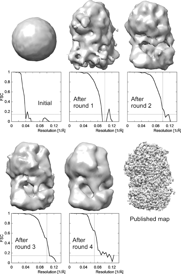
Example of an initial map generated from a reconstruction calculated using randomly assigned Euler angles. The dataset contained images of L protein of vesicular stomatitis virus (VSV-L) and led to a 3.8-Å reconstruction of this multi-enzyme (Liang et al., 2015). To initiate the startup procedure, the particle images was binned 3-fold to an effective pixel size of 3.711 Å and cropped to generate particle images of 60 × 60 pixels. A subset of 11,671 particles with an underfocus ranging between 1.7 and 2.5 µm were selected form the complete dataset (356,211 particles) and 40 rounds of multi-resolution search and refinement were performed according to the scheme described in Section 4.5, using five classes and starting with a resolution limit of 40 Å that was gradually increased to 10 Å resolution. FBOOST was set to T for this startup procedure. Reconstructions at each stage are shown together with the calculated FSC curves, starting with the initial map obtained with randomly assigned angles (labeled “Initial”). The reconstruction with the best FSC curve from each round was selected to seed the next round of refinement and classification. The FSC curve gradually improves from round to round until the final round 4 in which only 25 refinement cycles were run and the resolution was limited to 14 Å. The FSC curve for the final round indicates a resolution of about 9.5 Å according to the 0.143 criterion (Rosenthal and Henderson, 2003) indicated by the horizontal gray line, thus significantly exceeding the resolution limit used in the refinement (indicated by the vertical gray line) and therefore reflecting an unbiased resolution estimate. The FSC curves in earlier rounds likely reflects some bias as the resolution limit during refinement exceeded to resolution indicated by the FSC. The final published map is shown in the last panel for comparison.

4.6. Using masks

Frealign can employ two types of masks. The first involves a 3D volume stored in the same format as the input references. The mask file should contain positive and negative numbers outlining regions of the reference to be included or excluded by the mask, respectively. The mask file must be specified in mparameters using the mask_file key (if no filename is provided, Frealign assumes that a 3D mask is not used). Frealign will apply (i.e. multiply) the mask to the input references before starting refinement after making the following modifications to the mask file:

• all positive mask densities are reset to 1,

• all negative mask densities are reset to 0 or another value specified in mparameters, keyword mask_outside_weight,

• a soft edge is added to the mask (i.e. the region now containing voxels set to 1) using a width specified in pixels in mparameters, keyword mask_edge (usually set to 5),

• if specifying a value for mask_outside_weight larger than 0, the user can also specify if the density outside the mask should be low-pass filtered by setting keyword mask_filt_res to specify the filter resolution (a value of 0 turns the filter off) and mask_filt_edge to specify the width of a smooth edge (in units of Fourier voxels, usually set to 5) in mparameters.

This set of parameters provides the user with different masking strategies. Usually, the goal of masking will be to set all densities outside the mask to 0 and retain unmodified density inside the mask so that refinement and/or classification is driven solely by the density inside the mask. However, depending on the size of the particle and mask, the fraction of density left after masking may be too small to achieve reliable particle alignment. The result may be larger alignment errors and loss of resolution in the reconstructions. Using different combinations of mask_outside_weight and mask_filt_res, it is possible to retain density outside the mask that is downweighted and/or low-pass filtered to prevent significant particle misalignment against the masked references. Depending on the filtering and weighting, the alignment is still be driven by the density inside the mask at high resolution while particles are prevented from major misalignment by the low-resolution signal retained both inside and outside the mask. Users can experiment with different filtering and weighting applied to the density outside the mask to achieve the best results. Preventing misalignment when using masks can also be accomplished by turning off the refinement of some of the alignment parameters (see below).

The second type of masking does not require a 3D volume on input. Instead, using the keyword focus_mask in mparameters, the user specifies the coordinates and radius of a sphere that is then used by Frealign to mask regions in the particle images. Therefore, this second type of masking is applied to 2D images, not 3D volumes. For each particle image, the region inside the mask will be a disk that results from the thresholded projection of the specified sphere, in the direction of the view presented by the particle. This masking therefore depends on the correct alignment of the particles and should only be used once the alignments are reasonably accurate. The masked particle images will then be used to derive relative likelihood values that are used for classification (see above). The score function that is used for particle alignment is not affected by this type of masking and, therefore, the focus_mask option is only used for classification. Therefore, unlike with 3D masking, the alignment accuracy should remain as high as without masking.

By defining a sphere around a region of interest, only structural variability in this region will be used to classify particles. Since the mask is applied in 2D, parts of the volume overlapping with the region of interest in the views determined for the particles will be included inside the mask both in the particle image and projections of the reference structures. Differences between images and projections that drive classification will therefore result solely from true structural differences between the particles and references. This differs from 3D masking where density outside the masked region will also be missing in the projections of the masked reference structures. 2D masking may therefore increase the accuracy of classification, compared with 3D masking, an improvement that can also be achieved by subtracting constant parts of the 3D references from the particle images (Bai et al., 2015; Morais et al., 2003; Park et al., 2014) before determining their class memberships. However, unlike the approaches previously described, no shaped mask and no density subtraction in 2D or 3D is required. Masking in 2D offers the additional benefit of excluding noisy areas of the images that do not contain features to be classified, improving classification accuracy further. An example employing both 2D and 3D masking is shown in Fig. 6.

Figure 6.

Example of a classification scheme using 2D and 3D masking. The dataset consisted of 80S ribosomes prepared with the Taura syndrome virus internal ribosome entry site (TSV IRES) and elongation factor 2 (eEF2) (Abeyrathne et al, 2016). The complete dataset of 1,105,737 images of 80S•IRES•eEF2 complex was initially aligned against a density map calculated from the atomic model of the non-rotated 80S ribosome bound with 2 tRNAs (PDB: 3J78 (Svidritskiy et al., 2014)). This initial alignment was performed on data with a pixel size of 1.64 Å and limited to 20 Å resolution, resulting in a 3.5-Å resolution reconstruction. After five cycles of refinement the data were 2x binned (by Fourier cropping using the resample.exe tool, new pixel size = 3.28 Å) and subjected to classification into 15 classes using a 3D mask that contained the IRES, eEF2 and head domain of the small subunit. Six of the resulting classes (312,692 particle images) contained density for the IRES and eEF2 and were further classified into eight classes. For this classification, a 2D mask was applied around the ribosomal A site to include IRES pseudoknot I and eEF2 domain IV. The figure shows this mask as a sphere which, when projected according to the orientation of a particle, results in a 2D mask correctly placed on the region of interest. In the case of the 80S•IRES•eEF2 complex, this focused classification resulted in the separation of different translocation states of the IRES, catalyzed by eEF2, as shown schematically below each reconstruction. The states containing clear density for the IRES and eEF2 are highlighted in color.

The focus_mask option can be used to “explore” different regions of a particle and obtain different classification results depending on which region the sphere is placed in. This opens up the possibility of classification based on different particle regions that display uncorrelated heterogeneity. Each classification task focuses on only one of the affected regions and separates particles based on variability in this region. If variability in one region is correlated with that in another region, classification based on the former will also separate variable features in the latter. The focus_mask option can therefore be used to simplify a classification problem and to test if structural variability in different regions of the complex are correlated.

4.7. Asymmetric refinement

Symmetry present in a particle offers the advantage of additional averaging and the potential to increase the final resolution of a reconstruction. However, in many cases the individual particles will exhibit deviations from the nominal symmetry due to small distortions, disorder, conformational variability or the presence of pseudo symmetry that only becomes apparent at higher resolution. These deviations may limit the attainable resolution of the fully symmetrized reconstruction. One way to overcome this limitation is to treat the asymmetric subunits of each particle as separate entities (Ilca et al., 2015). Frealign provides an option to perform “asymmetric” refinement and reconstruction to explore if the alignment and classification of asymmetric units improves the density. To switch to the asymmetric reconstruction mode, users can change the letter of the symmetry symbol from upper case to lower case. For example, to carry out asymmetric refinement of a structure with nominal C2 symmetry, users must specify “c2” (keyword Symmetry in mparameters). In subsequent refinement cycles, additional lines will appear in the alignment parameter file with alignment results for each symmetry-related orientation of the particle. In the c2 example, there would be two lines of parameters for each particle, thus doubling the number of lines in the parameter file. In the reconstruction step, Frealign inserts particle images into the 3D volume according to each line in the parameter file, without applying additional symmetry. Therefore, if the alignment parameters on different lines belonging to the same particle differ, this will break the symmetry of the reconstruction. It is therefore possible to obtain a reconstruction that is not perfectly symmetrical when using asymmetric refinement.

The asymmetric mode can be used in two ways. In the first, particles with nominal symmetry experience distortion or disorder that displaces otherwise rigid subunits (or groups of subunits) from their symmetric positions. In this situation Frealign can align the subunits individually using a reference with an applied 3D mask (option mask_file, see above). For example, if a particle has a nominal C2 symmetry, a suitably designed 3D mask could be used to downweight or completely remove half of the reference density and align the particles against the remaining half. The particle images still contain both halves and Frealign will attempt to align each to the masked reference after applying symmetry-derived rotation matrices to transform each half into the correct frame of reference with respect to the masked reference. The resulting reconstruction should display improved density in the half of the reconstruction that survived the masking while the other half should display degraded density, depending on the amount of distortion/disorder present in the particles. It is important to note that the masking can also lead to increased alignment errors, degrading both halves of the density. Users should therefore carefully evaluate the asymmetric reconstructions and explore different masking options (see above).

The asymmetric refinement mode can also be used to classify symmetry-related regions (e.g. subunits) in a particle if these differ in their conformation or composition (e.g. ligand binding). In this case, classification (nclasses > 1, see above) has to be used together with asymmetric refinement. Using masking in 2D or 3D (see above), one of the symmetry-related regions has to be selected by the mask. Frealign will then assign each of the symmetry-related views of a particle to one of the classes using different occupancies in the alignment parameter file. In the resulting reconstructions, the region corresponding to the density inside the mask will contain the classification results while density outside this region will only show class-specific features if the variability inside the mask is correlated with that outside the mask.

Frealign currently does not offer a way to switch from asymmetric refinement back to regular refinement. Using their own scripts, users can reduce the “multi-line” parameter files to “single-line” parameter files to continue with regular refinement. As a technical note, the multiple alignment parameters for each particle do not include the additional symmetry-derived transforms that generate each of the symmetry-related views. This means that the alignment parameters in multi-line parameter files usually remain fairly similar to each other as differences only indicate the (typically small) differences in the alignments of the symmetry-related views.

4.8. Processing images of helical structures

Frealign includes an option to impose helical symmetry on reconstructions calculated from segments of helical structures and filaments (see chapter by Sachse). The helical symmetry can be selected using symmetry symbol “H” or “HP”. When “H” is specified, Frealign resets the alignment parameters at the beginning of a new refinement cycle to center all helical segments to be within a single “asymmetric unit” of the helical lattice. This will affect the Phi Euler angle, i.e. the third angle listed in the alignment parameter file that determines the rotation of each segment around the helical axis, and the x,y translations. While this is useful in most cases, it prevents the refinement and reconstruction of pseudo-helical structures, such as microtubules that have a seam. When symmetry “HP” is specified, the parameters are not reset and seam-sensitive alignments are preserved.

Frealign expects the helical axis to be aligned with the z-axis. The second Euler angle Theta, which describes the out-of-plane alignment of a helical segment, is therefore usually close to 90°. Most helical structures are also characterized by a persistence length that indicates how easy it is to bend them. The variability of the first Euler angle Psi, which describes the in-plane rotational alignment of a segment, is therefore limited depending on the value of the persistence length. While Frealign does not use persistence length as a parameter to restrict the angular alignment of segments, the user can define a STIFFNESS parameter as part of the helical symmetry section in mparameters. A large value for STIFFNESS will force the Psi and Theta angles to deviate less from the average values for a filament while a small value allows more variability. For this to work, it is important that segments belonging to the same filament are arranged consecutively in the alignment parameter file and image stack, and that the micrograph identifier (“Film” column in the parameter file) is the same for these segments. Other parameters that must be set when specifying helical symmetry are ALPHA (the rotation angle involved when going from one helical subunit to the next), RISE (the translation along the helical axis from one subunit to the next), NSUBUNITS (the number of unique subunits per segment; for overlapping segments that should only include the number of subunits in the non-overlapping parts) and NSTARTS (the number of helical starts present in the structure). Frealign provides a special mparameters template for helical image processing that includes these additional parameter keys. Users can access this template using the command frealign_helical_template. There is currently no option in Frealign to refine the helical symmetry parameters and users must therefore make sure that the ALPHA and RISE parameters are correct.

5. Tuning options

Frealign offers a number of tuning options that allows users to optimize refinement and classification. These options are typically used only after refinement with the standard (default) parameters has converged, i.e. no further improvement in the reconstructed density is observed when running additional refinement cycles. The following options, which are listed in the expert section in mparameters, are available:

• XSTD: determines if the input 3D reference should be masked (values larger than 0) or the 3D reference should be used to generate 2D masks (values smaller than 0) to be applied to the particle images before alignment (the masks are not used when calculating reconstructions). The default is 0, which disables this feature. Frealign interprets the provided value as a multiple of the standard deviation of the input 3D reference and values between 2 and 5 are usually appropriate. Higher values will tighten the masks while lower values will loosen them, both in 2D and 3D. Masking can reduce the noise present in the 3D reference or particle images but users must be careful not to overtighten the masks and cut into the 3D reference density or 2D particle density. 3D masking can also be achieved using the mask_file option (see above), which is preferred over the XSTD option because it provides the user with more control over different aspects of the masking.

• PBC: determines the weighting of individual particle images using a B-factor during reconstruction. The applied B-factor is calculated as B = 4 * score / PBC (in Ų). Reconstructions will be corrected for the average applied weights and therefore, only relative weight differences between particles are significant. A large value for PBC (e.g. 100) will effectively remove particle weighting while a small value (10 or smaller) will apply weighting. Users can recalculate reconstructions (using command frealign_calc_reconstructions) with different PBC values to see which value produces the best results.

• parameter_mask: determines which of the five alignment parameters (Psi, Theta and Phi Euler angles, x,y translations) will be refined. Normally, all parameters are refined and parameter_mask is set to “1 1 1 1 1”. However, any of these flags can be set to “0”, thereby forcing the corresponding parameter to remain constant during refinement. This allows users to reduce the degrees of freedom during refinement. For example, when images are collected as movies, it is possible to calculate movie sums with different numbers of frames, one with all frames to boost contrast and one with only the early frames to boost high resolution (Campbell et al., 2012). Frealign allows the use of different particle stacks for refinement and reconstruction by using the keywords raw_images_ref and raw_images_rec instead of raw_images. Using this simplified version of an exposure filter (Grant and Grigorieff, 2015b), it is possible to obtain higher resolution. However, if the movie frames are not accurately aligned there might be small differences in the translational alignments of the particles between the refinement and reconstruction stacks (rotational differences are usually very small and can be ignored). Once the best possible alignments have been obtained using the stack corresponding to a higher exposure, one or two additional refinement cycles using the low-exposure stack can increase the resolution even further. Since only translational alignment is needed, parameter_mask should be set to “0 0 0 1 1” to avoid increased errors in the Euler angles due to the lower image SNR of the low-exposure stack. Keeping some of the parameters constant may also be useful in other situations, for example when some of the alignment parameters are known from the experimental setup, such as in the random conical tilt (Radermacher et al., 1987) or orthogonal tilt reconstruction (Leschziner and Nogales, 2006) methods.

• thresh_reconst: determines the particle score value below which particles will be excluded from the reconstruction. Normally this value is set to 0 to include all particles. However, if a large fraction of particles are damaged or otherwise compromised and do not contribute high-resolution signal, reconstructions can be improved by excluding them. These particle images tend to receive lower scores than particles that contribute the stronges signal. Users can therefore tune their reconstructions by testing different values for thresh_reconst and recalculating the reconstruction (using command frealign_calc_reconstructions).

• FMATCH: specifies that Frealign should also output matching projections after each refinement cycle. The matching projections are stored inside Frealign’s scratch directory and will have names that include the pattern _reproject_. It is recommended to keep FMATCH set to “F” and use the command frealign_calc_projections instead to generate match projections, after refinement is completed. Inspecting matching projections may be useful to verify that particle alignment was successful, especially when starting without a set of alignment parameters and MODE set to 3 (see above).

• FBEAUT: if set to “T”, Frealign will apply the specified particle symmetry also in real space. This will not improve the results of the refinement but may improve the appearance of symmetry in a reconstruction if some of the symmetry operators require interpolation to be represented in the orthogonal coordinate system used by Frealign. The feature is therefore usually only used when making figures for presentations and publications.

• FBOOST: determines if a signed (when set to “T”) or an unsigned (when set to “F”) correlation coefficient is maximized during particle parameter refinement. As explained above, refining with the signed correlation coefficient may improve alignments but also increases the chance of overfitting. Users should initially refined with FBOOST set to “F” and, after convergence, test if additional refinement cycles with FBOOST set to “T” improve the reconstruction. It is important to limit the resolution used during refinement and look for a clear improvement of the FSC curve beyond the resolution limit. Also, an improvement of the FSC should be accompanied by an improvement in the density that can be correlated with known structural features. Users may have to sharpen the reconstructed density using bfactor.exe (see below) to observe high-resolution features.

• beam_tilt_x, beam_tilt_y: allows users to specify a beam tilt that Frealign will include during CTF correction. The values must be given in units of milliradians. Frealign cannot refine these values. However, if the presence of beam tilt is suspected, users can try different values and recalculate the reconstructions (using command frealign_calc_reconstructions) to find the best values.

• FMAG, FDEF, FASTIG, FPART: setting any of these flags to “T” will enable refinement of the magnification, defocus and astigmatism, optionally for individual particles (FPART set to “T”). Refinement of these parameters is usually not warranted, and users should not use these options in most cases.

• RBfactor: alters the correlation function used during refinement. This is not recommended and users should not use this option in most cases.

6. Related software

Besides Frealign, there are several other image processing tools that have been developed in the Grigorieff lab and that are freely available for download from the lab web page. Since some of these may be useful in combination with Frealign, they are briefly listed here for reference.

• Signature: software to display micrographs and select particles (Chen and Grigorieff, 2007). A semi-automatic mode is available that uses templates to identify particles using an algorithm first developed for FindEM (Roseman, 2004).

• CTFFIND3/CTFTILT: software used to determine accurate image defocus present in a micrograph (Mindell and Grigorieff, 2003) of untilted and tilted samples. A recent update, CTFFIND4, offers significant speedups over CTFFIND3 (Rohou and Grigorieff, 2015).

• BFACTOR: a tool to low-pass filter images and 3D density maps, and to estimate and apply a B-factor to bring out high-resolution features in a map. This tool is also included with the Frealign distribution.

• CROP: a tool to cut out a region of density from a 2D image or 3D volume.

• DIFFMAP: a tool to perform amplitude scaling of one 3D map against another and to write out a difference map. The tool can be used for scaling of 3D maps even if these are not aligned with each other. While the difference map is not meaningful in this case, the scaled maps should have similar filtering and B-factor sharpening, making it easier to compare them in terms of quality and high-resolution features.

• Unblur/Summovie: software to align frames of movies collected on an electron microscope, and to apply exposure-dependent filtering to the frames to enhance high-resolution signal (Grant and Grigorieff, 2015b).

• mag_distortion_estimate/correct: a tool to measure and correct for magnification distortions present in electron microscope images (Grant and Grigorieff, 2015a).

References

- Abeyrathne P, Koh CS, Grant T, Grigorieff N, & Korostelev AA (2016). Ensemble cryo-EM uncovers inchworm-like translocation of a viral IRES through the ribosome. Elife, in press. [DOI] [PMC free article] [PubMed]
- Alushin GM, Ramey VH, Pasqualato S, Ball DA, Grigorieff N, Musacchio A, et al. (2010). The Ndc80 kinetochore complex forms oligomeric arrays along microtubules. Nature 467, 805–810. [DOI] [PMC free article] [PubMed] [Google Scholar]
- Bai XC, Rajendra E, Yang G, Shi Y, & Scheres SH (2015). Sampling the conformational space of the catalytic subunit of human gamma-secretase. Elife 4. [DOI] [PMC free article] [PubMed] [Google Scholar]
- Campbell MG, Cheng A, Brilot AF, Moeller A, Lyumkis D, Veesler D, et al. (2012). Movies of ice-embedded particles enhance resolution in electron cryo-microscopy. Structure 20, 1823–1828. [DOI] [PMC free article] [PubMed] [Google Scholar]
- Chen JZ, & Grigorieff N (2007). SIGNATURE: a single-particle selection system for molecular electron microscopy. J Struct Biol 157, 168–173. [DOI] [PubMed] [Google Scholar]
- Crowther RA, Henderson R, & Smith JM (1996). MRC image processing programs. J Struct Biol 116, 9–16. [DOI] [PubMed] [Google Scholar]
- Frank J, Radermacher M, Penczek P, Zhu J, Li Y, Ladjadj M, et al. (1996). SPIDER and WEB: processing and visualization of images in 3D electron microscopy and related fields. J Struct Biol 116, 190–199. [DOI] [PubMed] [Google Scholar]
- Grant T, & Grigorieff N (2015a). Automatic estimation and correction of anisotropic magnification distortion in electron microscopes. J Struct Biol 192, 204–208. [DOI] [PMC free article] [PubMed] [Google Scholar]
- Grant T, & Grigorieff N (2015b). Measuring the optimal exposure for single particle cryo-EM using a 2.6 A reconstruction of rotavirus VP6. Elife 4, e06980. [DOI] [PMC free article] [PubMed] [Google Scholar]
- Grigorieff N (1998). Three-dimensional structure of bovine NADH:ubiquinone oxidoreductase (complex I) at 22 A in ice. J Mol Biol 277, 1033–1046. [DOI] [PubMed] [Google Scholar]
- Grigorieff N (2000). Resolution measurement in structures derived from single particles. Acta Crystallogr D Biol Crystallogr 56, 1270–1277. [DOI] [PubMed] [Google Scholar]
- Grigorieff N (2002). Single particles always fit the mold. Paper presented at: Frontiers in Structural Cell Biology: How Can We Determine the Structures of Large Subcellular Machines at Atomic Resolution? (Asilomar, California: The Biophysical Scociety)
- Grigorieff N (2007). FREALIGN: high-resolution refinement of single particle structures. J Struct Biol 157, 117–125. [DOI] [PubMed] [Google Scholar]
- Harauz G, & van Heel M (1986). Exact Filters for General Geometry 3-Dimensional Reconstruction. Optik 73, 146–156. [Google Scholar]
- Henderson R, Sali A, Baker ML, Carragher B, Devkota B, Downing KH, et al. (2012). Outcome of the first electron microscopy validation task force meeting. Structure 20, 205–214. [DOI] [PMC free article] [PubMed] [Google Scholar]
- Ilca SL, Kotecha A, Sun X, Poranen MM, Stuart DI, & Huiskonen JT (2015). Localized reconstruction of subunits from electron cryomicroscopy images of macromolecular complexes. Nat Commun 6, 8843. [DOI] [PMC free article] [PubMed] [Google Scholar]
- Kucukelbir A, Sigworth FJ, & Tagare HD (2014). Quantifying the local resolution of cryo-EM density maps. Nat Methods 11, 63–65. [DOI] [PMC free article] [PubMed] [Google Scholar]
- Leschziner AE, & Nogales E (2006). The orthogonal tilt reconstruction method: an approach to generating single-class volumes with no missing cone for ab initio reconstruction of asymmetric particles. J Struct Biol 153, 284–299. [DOI] [PubMed] [Google Scholar]
- Li X, Grigorieff N, & Cheng Y (2010). GPU-enabled FREALIGN: accelerating single particle 3D reconstruction and refinement in Fourier space on graphics processors. J Struct Biol 172, 407–412. [DOI] [PMC free article] [PubMed] [Google Scholar]
- Liang B, Li Z, Jenni S, Rameh AA, Morin BM, Grant T, Grigorieff N, Harrison SC & Whelan SPJ (2015). Structure of the L-protein of vesicular stomatitis virus from electron cryomicroscopy. Cell, 162, 314–327. [DOI] [PMC free article] [PubMed] [Google Scholar]
- Lyumkis D, Brilot AF, Theobald DL, & Grigorieff N (2013). Likelihood-based classification of cryo-EM images using FREALIGN. J Struct Biol 183, 377–388. [DOI] [PMC free article] [PubMed] [Google Scholar]
- Matthews BW (1968). Solvent content of protein crystals. J Mol Biol 33, 491–497. [DOI] [PubMed] [Google Scholar]
- Mindell JA, & Grigorieff N (2003). Accurate determination of local defocus and specimen tilt in electron microscopy. J Struct Biol 142, 334–347. [DOI] [PubMed] [Google Scholar]
- Morais MC, Kanamaru S, Badasso MO, Koti JS, Owen BA, McMurray CT, et al. (2003). Bacteriophage phi29 scaffolding protein gp7 before and after prohead assembly. Nat Struct Biol 10, 572–576. [DOI] [PubMed] [Google Scholar]
- Park E, Menetret JF, Gumbart JC, Ludtke SJ, Li W, Whynot A, et al. (2014). Structure of the SecY channel during initiation of protein translocation. Nature 506, 102–106. [DOI] [PMC free article] [PubMed] [Google Scholar]
- Pettersen EF, Goddard TD, Huang CC, Couch GS, Greenblatt DM, Meng EC, et al. (2004). UCSF Chimera--a visualization system for exploratory research and analysis. J Comput Chem 25, 1605–1612. [DOI] [PubMed] [Google Scholar]
- Radermacher M, Wagenknecht T, Verschoor A, & Frank J (1987). Three-dimensional reconstruction from a single-exposure, random conical tilt series applied to the 50S ribosomal subunit of Escherichia coli. J Microsc 146, 113–136. [DOI] [PubMed] [Google Scholar]
- Rohou A, & Grigorieff N (2015). CTFFIND4: Fast and accurate defocus estimation from electron micrographs. J Struct Biol 192, 216–221. [DOI] [PMC free article] [PubMed] [Google Scholar]
- Roseman AM (2004). FindEM--a fast, efficient program for automatic selection of particles from electron micrographs. J Struct Biol 145, 91–99. [DOI] [PubMed] [Google Scholar]
- Rosenthal PB, & Henderson R (2003). Optimal determination of particle orientation, absolute hand, and contrast loss in single-particle electron cryomicroscopy. J Mol Biol 333, 721–745. [DOI] [PubMed] [Google Scholar]
- Sindelar CV, & Grigorieff N (2012). Optimal noise reduction in 3D reconstructions of single particles using a volume-normalized filter. J Struct Biol 180, 26–38. [DOI] [PMC free article] [PubMed] [Google Scholar]
- Stewart A, & Grigorieff N (2004). Noise bias in the refinement of structures derived from single particles. Ultramicroscopy 102, 67–84. [DOI] [PubMed] [Google Scholar]
- Svidritskiy E, Brilot AF, Koh CS, Grigorieff N, and Korostelev AA (2014). Structures of Yeast 80S Ribosome-tRNA Complexes in the Rotated and Nonrotated Conformations. Structure 22, 1210–1218. [DOI] [PMC free article] [PubMed] [Google Scholar]
- van Heel M, Harauz G, Orlova EV, Schmidt R, & Schatz M (1996). A new generation of the IMAGIC image processing system. J Struct Biol 116, 17–24. [DOI] [PubMed] [Google Scholar]
- Wolf M, DeRosier DJ, & Grigorieff N (2006). Ewald sphere correction for single-particle electron microscopy. Ultramicroscopy 106, 376–382. [DOI] [PubMed] [Google Scholar]
- Yang Z, Fang J, Chittuluru J, Asturias FJ, & Penczek PA (2012). Iterative stable alignment and clustering of 2D transmission electron microscope images. Structure 20, 237–247. [DOI] [PMC free article] [PubMed] [Google Scholar]