Abstract
Cervical cancer, which has been affecting women worldwide as the second most common cancer, can be cured if detected early and treated well. Routinely, expert pathologists visually examine histology slides for cervix tissue abnormality assessment. In previous research, we investigated an automated, localized, fusion-based approach for classifying squamous epithelium into Normal, CIN1, CIN2, and CIN3 grades of cervical intraepithelial neoplasia (CIN) based on image analysis of 61 digitized histology images. This research introduces novel acellular and atypical cell concentration features computed from vertical segment partitions of the epithelium region within digitized histology images to quantize the relative increase in nuclei numbers as the CIN grade increases. Based on CIN grade assessments from two expert pathologists, image-based epithelium classification is investigated with voting fusion of vertical segments using support vector machine (SVM) and Linear Discriminant Analysis (LDA) approaches. Leave-one-out is used for training and testing for CIN classification, achieving an exact grade labeling accuracy as high as 88.5%.
Keywords: Cervical cancer, cervical intraepithelial neoplasia, fusion-based classification, image processing, linear discriminant analysis, support vector machine
I. Introduction
In 2008, there were 529,000 new cases of invasive cervical cancer reported worldwide. [1]. While the greatest impact of cervical cancer prevalence is in the developing world, invasive cervical cancer continues to be diagnosed in the US each year. Detection of cervical cancer and its precursor lesion is accomplished through a Pap test, a colposcopy to visually inspect the cervix, and microscopic interpretation of histology slides by a pathologist when biopsied cervix tissue is available. Microscopic evaluation of histology slides by a qualified pathologist has been used as a standard of diagnosis [2]. As part of the pathologist diagnostic process, cervical intraepithelial neoplasia (CIN) is a pre-malignant condition for cervical cancer in which the atypical cells are identified in the epithelium by the visual inspection of histology slides [3]. As shown in Fig. 1, cervical biopsy diagnoses include normal (that is, no CIN lesion), and three grades of CIN: CIN1, CIN2 and CIN3 [3][4][5]. CIN1 corresponds to mild dysplasia (abnormal change), whereas CIN2 and CIN3 are used to denote moderate dysplasia and severe dysplasia, respectively. Histologic criteria for CIN include increasing immaturity and cytologic atypia in the epithelium.
Fig. 1.
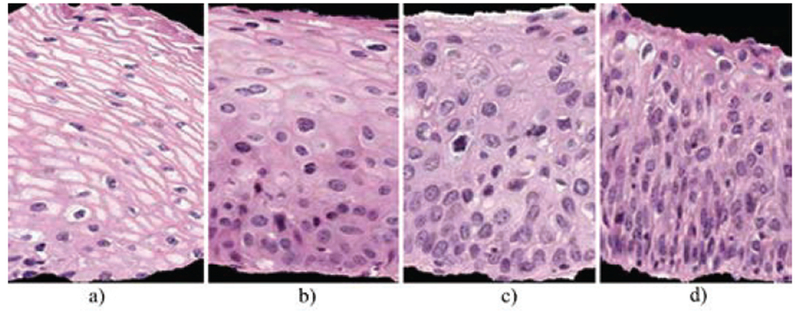
CIN grade label examples highlighting the increase of immature atypical cells from epithelium bottom to top with increasing CIN severity. (a) Normal, (b) CIN 1, (c) CIN 2, (d) CIN 3.
As CIN increases in severity, the epithelium has been observed to show delayed maturation with an increase in immature atypical cells from bottom to top of the epithelium [4][5][6][7]. As shown in Fig. 1, atypical immature cells are seen mostly in the bottom third of the epithelium for CIN 1 (Fig. 1b). For CIN2, the atypical immature cells appear in the bottom two thirds of the epithelium (Fig. 1c), and, for CIN 3, atypical immature cells lie in the full thickness of the epithelium (Fig. 1d). When these atypical cells extend beyond the epithelium, that is, through the basement membrane and start to enter into the surrounding tissues and organs, it may indicate invasive cancer [3]. In addition to analyzing the progressively increasing quantity of atypical cells from bottom to top of the epithelium, identification of nuclei atypia is also significant [3]. Nuclei atypia is characteristic of nuclei enlargement, thereby resulting in different shapes and sizes of the nuclei present within the epithelium region. Visual assessment of this nuclei atypia may be difficult, due to the large number of nuclei present and the complex visual field, that is, tissue heterogeneity. This may contribute to diagnostic grading repeatability problems and inter- and intra-pathologist variation [6][7][8].
Computer-assisted methods (digital pathology) have been explored for CIN diagnosis in other studies [5][9][10][11][12] and provided the foundation for the work reported in [9]. These methods examined texture features [11], nuclei determination and Delaunay triangulation analysis [12], medial axis determination [5], and localized CIN grade assessment [5]. A more detailed review of digital pathology techniques is presented in that paper [9]. Our research group previously investigated a localized, fusion-based approach to classify the epithelium region into the different CIN grades, as determined by an expert pathologist [9]. We examined 66 features including texture, intensity shading, Delaunay triangle features (such as area and edge length), and Weighted Density Distribution (WDD) features, which yielded an exact CIN grade label classification result of 70.5% [9].
The goal of this research, performed in collaboration with the National Library of Medicine (NLM), is to automatically classify sixty-one manually segmented cervical histology images into four different grades of CIN and to compare results with CIN grade determination by an expert pathologist. The research presented in this paper extends the study in [9] to the development of new image analysis and classification techniques for individual vertical segments to allow improved whole-image CIN grade determination. Specifically, we present new image analysis techniques to determine epithelium orientation and image analysis and to find and characterize acellular and nuclei regions within the epithelium. We also present comparative CIN grading classification analysis vs. two expert pathologists CIN grading of the sixty-one image data set.
The order of the remaining sections of the article is as follows: Section II presents the methods used in this research; Section III describes the experiments performed; Section IV presents and analyzes the results obtained and a discussion; Section V provides the study conclusions.
II. Methods
The images analyzed included 61 full-color digitized histology images of hematoxylin and eosinophil (H&E) preparations of tissue sections of normal cervical tissue and three grades of cervical carcinoma in situ. An additional image, labeled as CIN1 by two experts (RZ and SF), was used for image processing algorithm parameter determination. The same experimental data set was used in [9]. The entire classification process, as utilized in [9], of the segmented epithelium images was performed using the following five-step approach:
Step 1: Locate the medial axis of the segmented epithelium region;
Step 2: Divide the segmented image into ten vertical segments, orthogonal to the medial axis;
Step 3: Extract features from each of the vertical segments;
Step 4: Classify each of these segments into one of the CIN grades;
Step 5: Fuse the CIN grades from each vertical segment to obtain the CIN grade of the whole epithelium for image-based classification.
The following sections present each step in detail.
A. Medial Axis Detection and Segments Creation
Medial axis determination used a distance transform-based [13][14] approach from [9]. The distance transform-based approach from [9] had difficulties finding the left- and right-hand end-axis portions of the epithelium axis in nearly rectangular and triangular regions. Fig. 2 shows an example of an incorrect medial axis estimation using a distance-transform based approach (solid line) and the manually labeled desired medial axis (dashed line).
Fig. 2.
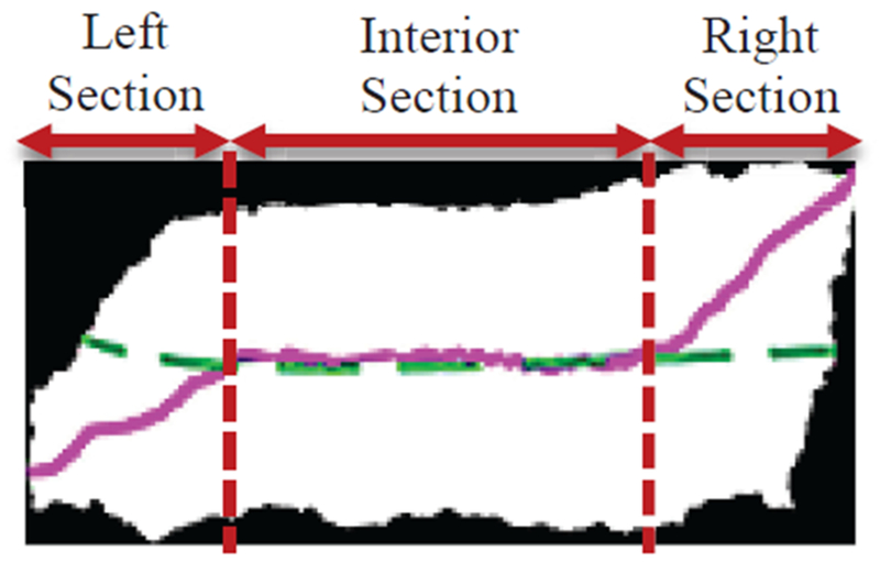
Example of incorrect medial axis determined using distance transform only (solid line). The desired medial axis is manually drawn and is overlaid on the image (dashed line). The left-hand, right-hand, and interior sections are labeled on the bounding box image to highlight the limitations of the distance transform algorithm.
Accordingly, the algorithm from [9] used the bounding box of the epithelium to obtain a center line through the bounding box and intersecting the center line with the epithelium object. The resulting center line was divided into a left-hand segment (20%), a right-hand segment (20%), and the interior segment (60%). These divisions of the epithelium can be observed in Fig. 2. The interior 60% portion of the distance transform-based medial axis was retained as part of the final medial axis. The left- and right-hand cutoff points of the interior distance transform axis were determined as the closest Euclidean distance points from the distance transform axis to the center line points on the 20% left- and right-hand segments. As done in [9], the left- and right-hand cutoff points are projected to the median bounding box points for the remaining left-hand 20% and right-hand 20% portions of the axis. The projected left- and right-hand segments are connected with the interior distance transform axis to yield the final medial axis.
The epithelium’s orientation was determined using a novel approach based on the bounding box and the final medial axis. Using the bounding box, a comparison was performed of the number of nuclei distributed over eight masks that are created from eight control points (P1, P2, P3,…, P8) at the corners and midpoints of the bounding box edges (Fig. 3).
Fig. 3.

Bounding box of epithelium with control points labeled.
The masks are used for computing the ratios of the number of detected nuclei to the areas of the masks. The control points used for determining the masks are shown as P1 through P8 in Fig. 3. For each control point combination, the number of nuclei is computed for each mask using the algorithm presented in section II.B.1 below. Let n represent the set of the number of nuclei computed from masks 1-8, given as n = {n1, n2, …, n8] as designated in Fig. 4 a-d. The eccentricity, defined as the ratio of the fitted ellipse foci distance to the major axis length as given in [16], is computed for the entire epithelium image mask, given as e, and for each mask image, denoted as ei. Then, the eccentricity weighted nuclei ratios are calculated for each mask combination, given as v = {v12, v34, v56, v78, v21, v43, v65, v87}, Where… , , , , etc., and max(n) denotes the maximum area of the 8 partitioned masks. The term ni/max(n) is used as a scale factor for normalizing the size of the epithelium region. The medial axis top/bottom orientation is determined as vij = maxij(v). The resulting medial axis is partitioned into ten segments of approximately equal length, perpendicular line slopes are estimated at the mid-points of each segment, and vertical lines are projected at the end points of each segment to generate ten vertical segments for analysis. The partitioning of the epithelium image into ten vertical segments was performed to facilitate localized CIN classifications within the epithelium that can be fused to provide an image-based CIN assessment, as done in [9], Fig. 5 provides an example of the medial axis partitioning and the ten vertical segments obtained.
Fig. 4.
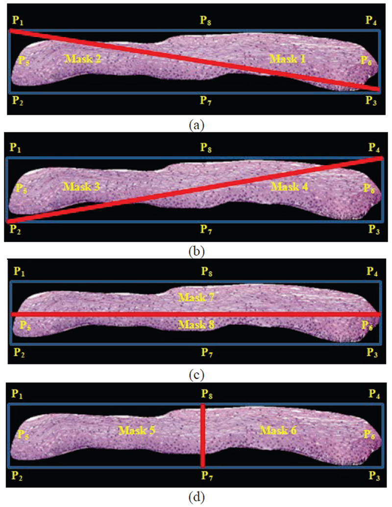
Bounding box partitioning with masks combinations shown based on control points from Figure 3 as part of epithelium orientation determination algorithm. (a) Mask 1 & Mask 2. (b) Mask 3 & Mask 4. (c) Mask 5 & Mask 6. (d) Mask 7 & Mask 8.
Figure 5:
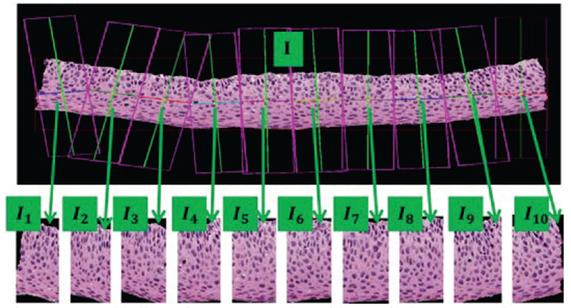
Epithelium image example with vertical segment images (I1, I2, I3,…, I10) determined from bounding boxes after dividing the medial axis into ten line segment approximations after medial axis computation.
B. Feature Extraction
Features are computed for each of the ten vertical segments of the whole image, I1, I2, I3, …, I10. All the segments of one whole image are feature-extracted in a sequence, from left to right, I1 to I10, (Fig. 5).
In total, five different types of features were obtained in this research, including: 1) Texture features (F1-F10) [9], 2) Cellularity features (F11-F13), 3) Nuclei features (F14,F15), 4) Acellular (light area) features (F16-F22), 4) Combination features (F23,F24) and 5) Advanced layer-by-layer triangle features (F25-F27). To give a brief introduction of the extracted features, Table 1 is presented showing the feature label and brief description in every row for each feature.
Table I.
Feature Description
| Label | Description |
|---|---|
| F1 | Contrast of segment: Intensity contrast between a pixel and its neighbor over the segment image. |
| F2 | Energy of segment: Squared sum of pixel values in the segment image. |
| F3 | Correlation of segment: How correlated a pixel is to neighbors over the segment image. |
| F4 | Segment homogeneity: Closeness of the distribution of pixels in the segment image to the diagonal elements. |
| F5, F6 | Contrast of GLCM: Local variation in GLCM in horizontal and vertical directions |
| F7, F8 | Correlation of GLCM: Joint probability occurrence (periodicity) of elements in the segment image in the horizontal and vertical directions |
| F9, F10 | Energy of GLCM: Sum of squared elements in the GLCM in horizontal and vertical directions. |
| F11 | Acellular ratio: Proportion of object regions within segment image with light pixels (acellular). |
| F12 | Cytoplasm ratio: Proportion of object regions within segment image with medium pixels (cytoplasm). |
| F13 | Nuclei ratio: Proportion of object regions within segment image with dark pixels (nuclei). |
| F14 | Average nucleus area: Ratio of total nuclei area over total number of nuclei |
| F15 | Background to nuclei area ratio: Ratio of total background area to total nuclei area |
| F16 | Intensity ratio: Ratio of average light area image intensity to background intensity |
| F17 | Ratio R: Ratio of average light area red to background red |
| F18 | Ratio G: Ratio of average light area green to background green |
| F19 | Ratio B: Ratio of average light area blue to background blue |
| F20 | Luminance ratio: Ratio of average light area luminance to background luminance |
| F21 | Ratio light area: Ratio of light area to total area |
| F22 | Light area to background area ratio: Ratio of total light area to background area |
| F23 | Ratio acellular number to nuclei number: Ratio of number of light areas to number of nuclei |
| F24 | Ratio acellular area to nuclei area: Ratio of total light area to total nuclei area |
| F25 | Triangles in top layer: Number of triangles in top layer |
| F26 | Triangles in mid layer: Number of triangles in middle layer |
| F27 | Triangles in bottom layer: Number of triangles in bottom layer |
1. Texture and Cellular Features
The texture and color features were used in our previous work and are described in [9]. The use of color in histopathological image analysis is also described in [10][11]. For texture features, both first-order structural measures derived directly from the image segment and second-order statistical methods based on the gray-level co-occurrence matrix (GLCM) [5][18] were employed. A grayscale luminance version of the image was created in order to compute statistics of energy, correlation, contrast and uniformity of the segmented region; these statistics are then used to generate features (F1-F10) shown in Table 1. The texture features include contrast (F1), energy (F2), correlation (F3) and uniformity (F4) of the segmented region, combined with the same statistics (contrast, energy and correlation) generated from the GLCM of the segment (F5-F10, see Table 1).
The luminance images showed regions with three different intensities, marked as light, medium and dark areas within each single segmented luminance image, as shown in Fig. 6 of normal cervical histology. The light areas correspond to acellular areas; the medium areas correspond to cytoplasm, and the dark areas correspond to nuclei.
Fig. 6:
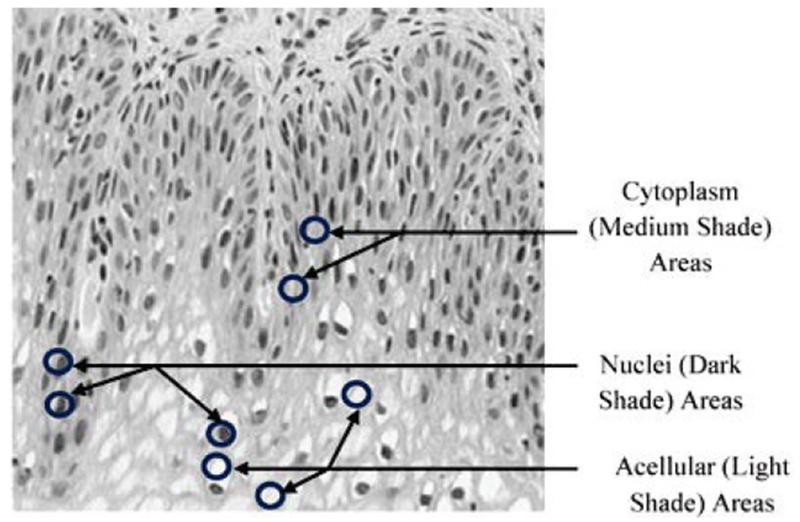
Sample shading representatives within epithelium image used for determining cellular features.
Cluster centers are found from the luminance image using K-means clustering [9] for three different regions (K = 3) denoted as clustLight clustMedium, and clustDark for the light, medium and dark cluster centers, respectively. Then the ratios are calculated based on Equations (1),(2), and (3) [9].
| (1) |
| (2) |
| (3) |
where Acellular ratio (F11), Cytoplasm ratio (F12) and Nuclei ratio (F13) represent the cellular features in Table 1, and numLight, numMedium, and numDark represent the number of pixels that were assigned to the clusters of light, medium and dark, respectively. These features correspond to Intensity Shading features developed in [9].
2. Nuclei Features
The dark shading color feature discussed above corresponds to nuclei, which appear within epithelial cells in various shapes and sizes. Nuclei tend to increase in both number and size as the CIN level increases. This linkage between nuclei characteristics and CIN levels motivates our development of algorithms for nuclei detection feature extraction. In this research, the algorithms of nuclei detection and nuclei feature extraction are developed to obtain features to facilitate CIN classification. Specifically, we carry out the following steps:
Nuclei feature pre-processing: average filter, image sharpening and histogram equalization.
Nuclei detection: clustering, hole filling, small-area elimination, etc.
Nuclei feature extraction.
In pre-processing, vertical image segments are processed individually. After converting the segment into a grayscale image I, an averaging filter is applied as in Equation (4) where * denotes convolution.
| (4) |
After the average-filtered image is obtained, an image sharpening method is used to emphasis the dark shading part which is expressed as Equation (5) following the methods in [17]:
| (5) |
where Isharpen is the sharpened image, and k is an empirically determined constant of 2.25. The average-filtered image A and the sharpened image Isharpen are shown in Fig. 8. In the final pre-processing step, we apply histogram equalization using the Matlab function histeq to the sharpened image (Isharpen) (in particular, to enhance details of the nuclei atypia).
Fig. 8:
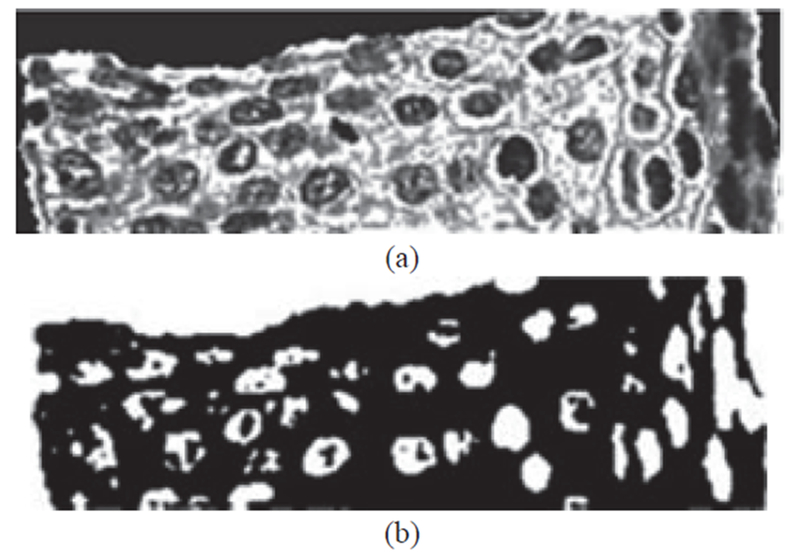
Example of image processing steps to obtain nuclei cluster pixels from K-Means algorithm from histogram equalized image. (a) Histogram equalized image determined from Fig. 7 (b). (b) Mask image obtained from K-means algorithm with pixels closest to nuclei cluster.
The nuclei detection algorithm is described as follows using the equalized histogram image as the input.
Step 1: Cluster the histogram-equalized image into clusters of background (darkest), nuclei, and darker and lighter (lightest) epithelium regions using the K-means algorithm (K = 4). Generate a mask image containing the pixels closest to the nuclei cluster (second darkest).
Step 2: Use the Matlab function imclose with a circular structuring element of radius 4 to perform morphological closing on the nuclei mask image.
Step 3: Fill the holes in the image from step 2 with Matlab’s imfill function for this process.
Step 4: Use the Matlab’s imopen to perform morphological opening with a circular structuring element of radius 4 on the image from step 3.
Step 5: Eliminate small area noise objects (non-nuclei objects) within the epithelium region of interest from the mask in step 4, with the area opening operation using the Matlab function bwareaopen.
Fig. 8 shows an example of a sharpened image before and after histogram equalization, which is input to the nuclei detection algorithm, and the resulting mask image with pixels closest to the nuclei cluster from the K-means algorithm in step 1. The nuclei detection algorithm steps 2-5 are illustrated in Fig. 9.
Fig. 9:
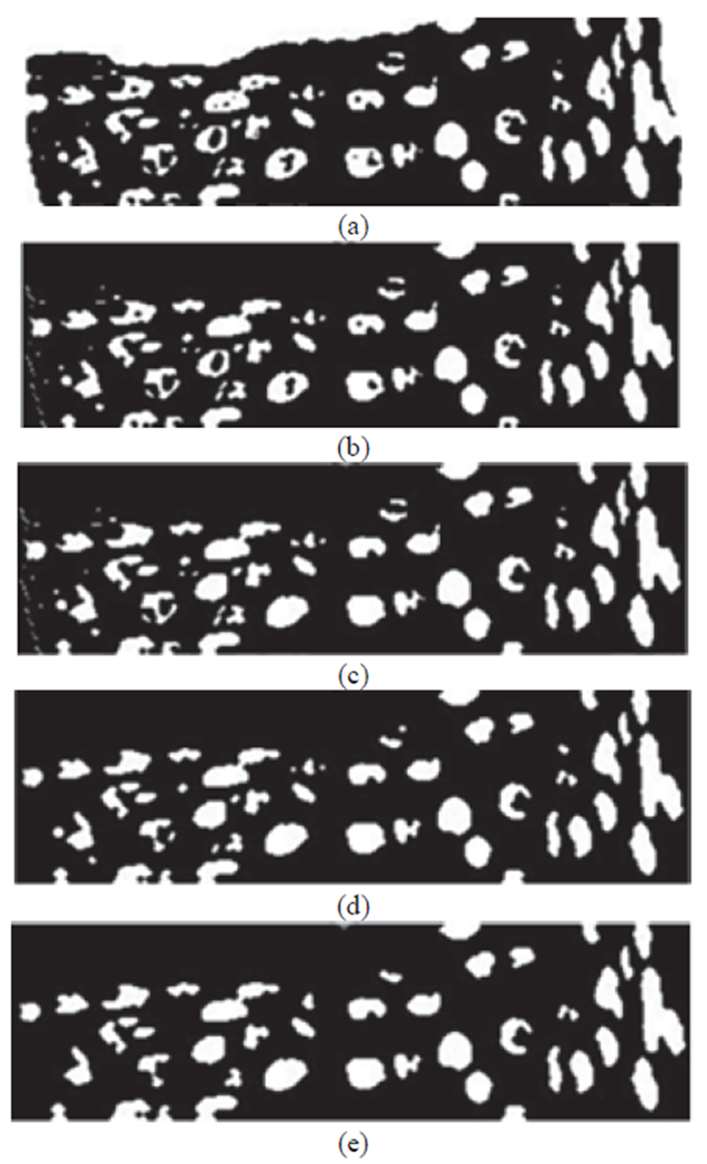
Image examples of nuclei detection algorithm. (a) Image with preliminary nuclei objects obtained from clustering (step 1 – Figure 8(c)). (b) Image closing to connect nuclei objects (step 2). (c) Image with hole filling to produce nuclei objects (step 3). (d) Image opening to separate nuclei objects (step 4). (e) Image with non-nuclei (small) objects eliminated (step 5).
The nuclei features are calculated as follows: With detected nuclei shown as white objects in the final binary images (Fig. 9e), the nuclei features are calculated as:
| (6) |
| (7) |
where Average nucleus area (F14) and Ratio of background to nuclei area (F15) represent ratios obtained from the final nuclei images, as shown in Fig. 9e. In (6) and (7), NucleiArea represents the total area for all nuclei detected (all white pixels); NucleiNumber indicates the total number of white regions (number of objects in Fig. 9e); AverageNucleusArea is the ratio of nuclei area to the nuclei number, which tends to increase with higher CIN grade; NonNucleiArea area represents the total number of pixels in the black non-nucleus region within the epithelium region (black pixels within epithelium in Fig. 9e). RatioBackgroundNucleusArea denotes the ratio of the non-nuclei area to nuclei area. We expect larger values of AverageNucleusArea to correspond to increasing CIN grade, and RatioBackgroundNucleusArea to decrease with increasing CIN grade.
3. Acellular Features
Extracting the light area regions, described previously as “light shading”, is challenging, due to the color and intensity variations in the epithelium images. We evaluated each of the L*-, a*-, and b*-planes of CIELAB color space for characterizing the light areas, and determined empirically that L* provides the best visual results. The following outlines the methods we used to segment the histology images:
Step 1: Convert the original image from RGB color space to L*a*b* color space, then select the luminance component L* (see Fig. 10).
Step 2: Perform adaptive histogram equalization on the image from step 1 using Matlab’s adapthisteq. adapthisteq operates on small regions (tiles) [15] for contrast enhancement so that that the histogram of the output region matches a specified histogram and combines neighboring tiles using bilinear interpolation to eliminate artificially induced boundaries (see Fig. 11).
Step 3: After the image has been contrast-adjusted, the image is binarized by applying an empirically determined threshold of 0.6. This step is intended to eliminate the dark nuclei regions and to retain the lighter nuclei and epithelium along with the light areas (see Fig. 12).
Step 4: Segment the light areas using the K-means algorithm based on [9], with K equal to 4. The K-means algorithm input is the histogram-equalized image from step 2 multiplied by the binary thresholded image from step 3. A light area clustering example is given in Fig. 13.
Step 5: Remove from the image all objects have an area less than 100 pixels, determined empirically, using the Matlab function regionprops [15]. A morphological closing is performed with a disk structure element of radius 2. An example result is shown in Fig. 14.
Fig. 10:
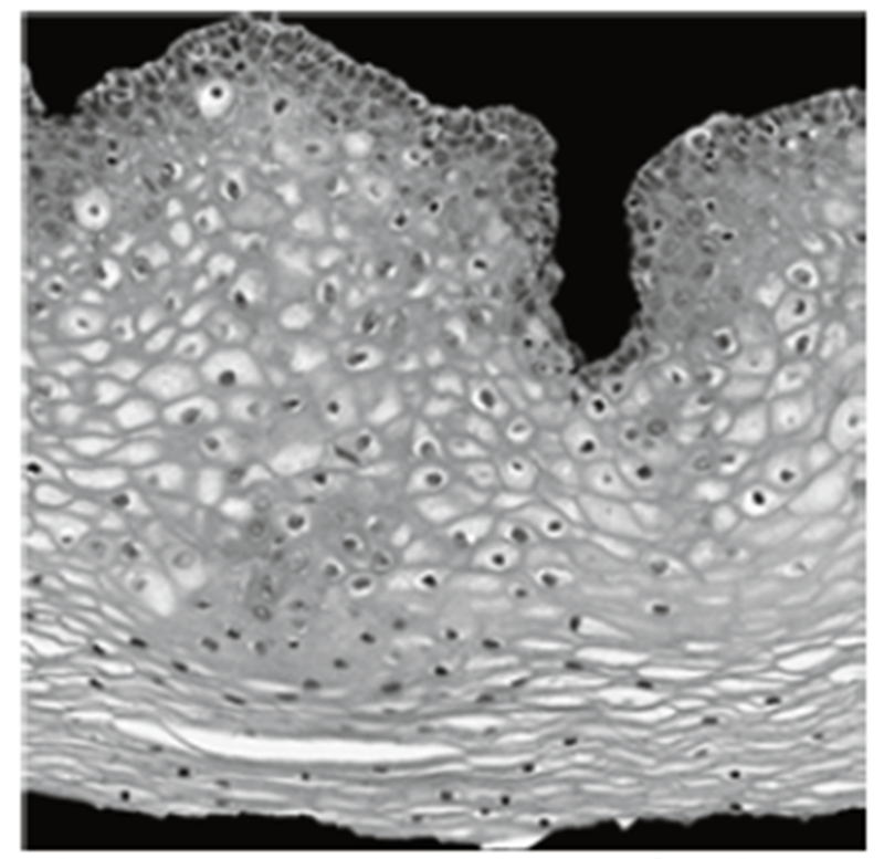
Example L* image for light area detection.
Fig. 11:
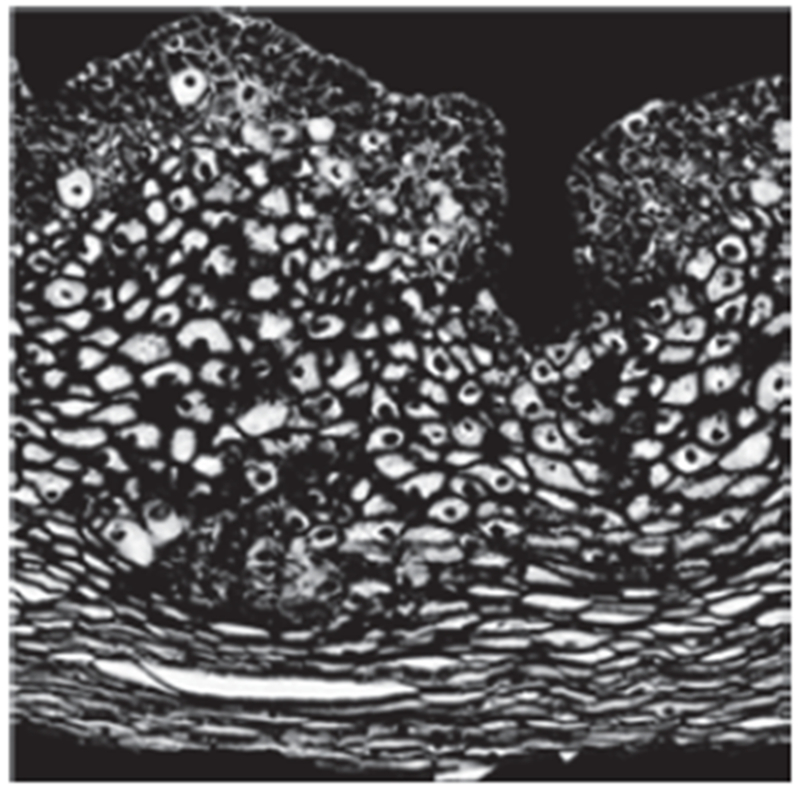
Adaptive histogram equalized image of Fig. 10.
Fig. 12:
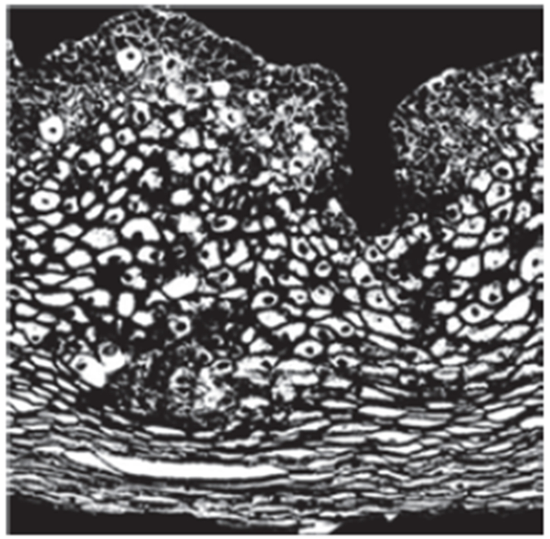
Thresholded image of Fig. 11.
Fig. 13:
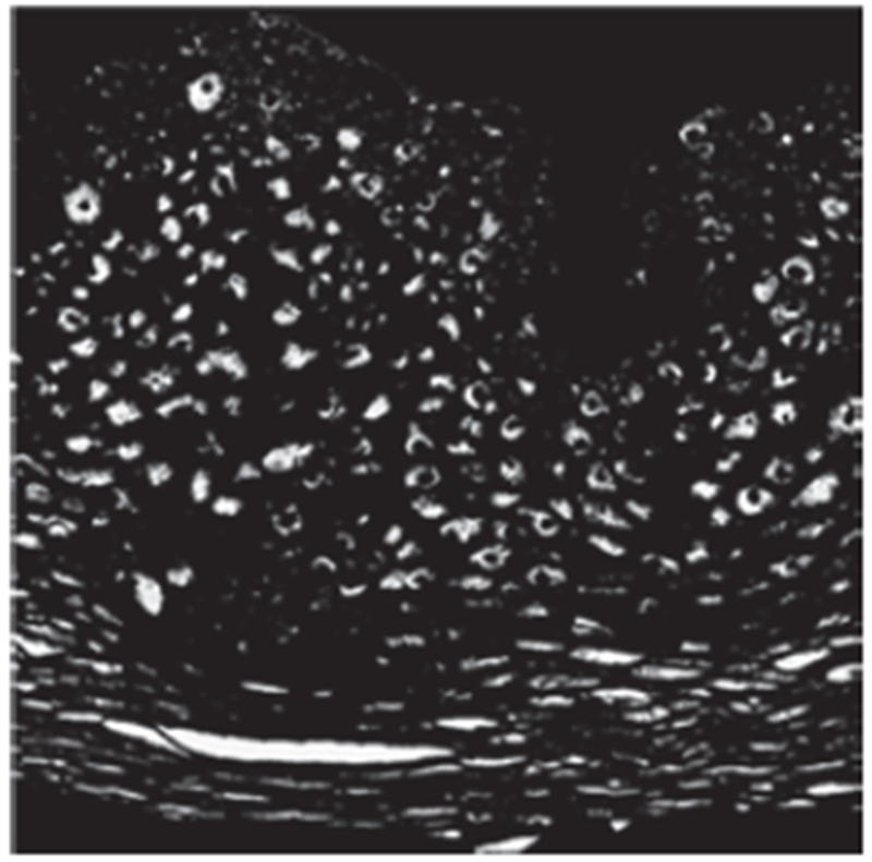
Example image of light area clusters after K-means clustering.
Fig. 14:
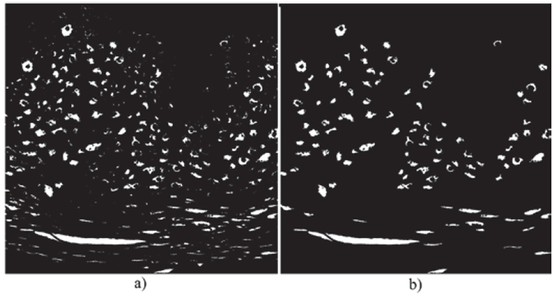
Example morphological dilation and final light area mask. (a) Morphological dilation and erosion process after K-means clustering (b) Final light area mask, after eliminating regions with areas smaller than 100 pixels.
Using the light area mask, the acellular features (from Table 1) are computed and given in (8)–(14) below:
| (8) |
| (9) |
| (10) |
| (11) |
| (12) |
| (13) |
| (14) |
where SegmentArea gives the epithelium area within the vertical segment; LightArea denotes the area of all light area regions; LightNumber corresponds to number of light areas; BackgroundArea represents the total number of non-nuclei and non-light area pixels inside the epithelium within the vertical segment (i.e., background area); LightAreaIntensity, LightAreaRed, LightAreaGreen, LightAreaBlue, and LightAreaLuminance are the average intensity, red, green, blue, and luminance values, respectively, of the light areas within epithelium of the vertical segment; BackgroundIntensity, BackgroundRed, BackgroundGreen, BackgroundBlue, and BackgroundLuminance are the average intensity, red, green, blue, and luminance values, respectively, of the non-nuclei and non-light area pixels within the epithelium of the vertical segment.
4. Combination features
After both the nuclei features and the acellular features were extracted, two new features were calculated with the intent to capture the relative increase in nuclei numbers as CIN grade increases. These features are the ratio of the acellular number to the nuclei number (F23), and the ratio of the acellular area to the total nuclei area (F24). The equations for calculating the combination features are presented below in (15) and (16):
| (15) |
| (16) |
where LightNumber and NucleiNumber represent the total number of light area and nuclei objects, respectively, as found in sections 2.2.2 and 2.2.3 (Fig. 6).
5. Triangle Features
In previous research, triangle features have been investigated based on the Circular-Hough Transform (CHT) [18] to detect nuclei for use as vertices in Delaunay triangle (DT) formulation [19] to obtain the triangles [9][10]. Features were computed which included triangle area and edges length, and simple statistics (means, standard deviations) of these quantities were also included as features. In applying the CHT to our experimental data set, we observed that for some images, this method sometimes fails to locate non-circular, irregularly-shaped nuclei; on the other hand, this method does (incorrectly) detect some non-nuclei regions as nuclei, which leads to incorrect vertices being input to the (DT) method, thus degrading the triangle features calculated in downstream processing. To overcome the shortcomings of the CHT for nuclei detection, we use the centroids of the nuclei detected based on the method presented in section II.B.2 (Nuclei Feature). An example comparison between the previous Circular-Hough method and the method in this paper is presented in Fig. 15. Circles indicate the locations of detected nuclei.
Fig. 15:
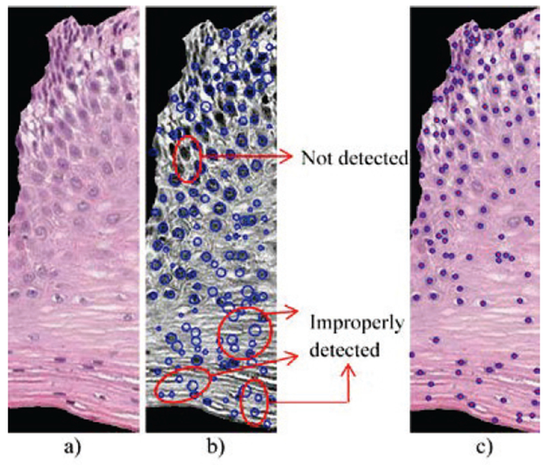
Example of nuclei detection comparison between the Circular-Hough method and the method presented in this paper. (a) The original vertical segment. (b) Example of Circular-Hough method; note the nuclei misses and false detections. (c) Nuclei detected using the algorithm from the Nuclei Features section.
In this research, we use the Delaunay triangle method, but restrict the geometrical regions it can act upon, as follows. Before forming the Delaunay triangles with the vertices provided by the nuclei detection results from Nuclei Feature section, the vertical segment being processed is sub-divided into three vertical layers, as illustrated in Fig. 16. The aim is to associate the presence of increasing nuclei throughout the epithelium with increasing CIN grades, namely: abnormality of the bottom third of the epithelium roughly corresponds to CIN1; abnormality of the bottom two-thirds, to CIN2; and abnormality of all three layers, to CIN3. We refer to these layers as bottom, mid, and top. (see Fig. 16, the green circles stand for the top layer vertices, red for mid layer and blue for bottom).
Fig. 16:
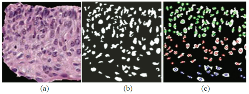
The distribution of nuclei centroids as vertices for Delaunay triangles in bottom layer (green), mid layer (red) and top layer (blue).
After locating the vertices for Delaunay triangles (DT), the DT algorithm iteratively selects point triples to become vertices of each new triangle created. Delaunay Triangulation exhibits the property that no point lies within the circles that are formed by joining the vertices of the triangles [5]. As shown in Fig. 17, all the triangles in three layers formed using DT are unique and do not contain any points within the triangles. The features are obtained according to the triangles in three different layers, including: number of triangles in top layer (F25), number of triangle in middle layer (F26) and number of triangles in bottom layer (F27).
Fig. 17:
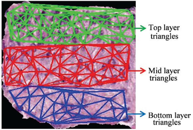
The Delaunay triangles in bottom layer (green lines), mid layer (red lines) and top layer (blue lines).
III. Experiments Performed
We carried out three sets of experiments, which are described in this section. The experimental data set consisted of 61 digitized histology images, which were CIN labeled by two experts (RZ and SF) (RZ: 16 Normal, 13 CIN1, 14 CIN2, and 18 CIN3; SF: 14 Normal, 14 CIN1, 17 CIN2, and 16 CIN3).
A. Fusion Based CIN Grade Classification of Vertical Segment Images
For the first set of experiments, all the features extracted from the vertical segment images were used as inputs to train the SVM/LDA classifier. The LIBSVM [22] implementation of the SVM and LDA classifiers were utilized in this study. The SVM implementation uses a linear kernel and the four weights were the fractions of the images in each CIN class to the entire image set (fraction of the image set that is Normal, fraction of the image set that is CIN1, etc.).
Individual features were normalized by subtracting the mean training set feature value and dividing by the standard deviation training set feature value. Due to the limited size of the image set, a leave-one-image-out approach was investigated for classifier training and testing. For this approach, the classifier is trained based on the individual vertical segment feature vectors for all but the left-out epithelium image (used as the test image). For classifier training, the expert truthed CIN grade for each image was assigned to the ten vertical segments for that image. For the left-out test image, each vertical segment was classified into one of the CIN grades using the SVM/LDA classifier.
Then, the CIN grades of the vertical segment images were fused to obtain the CIN grade of the entire test epithelium image (see Fig. 5). The fusion of the CIN grades of the vertical segment images was completed using a voting scheme. The CIN grade of the test epithelium image was assigned to the most frequently occurring class assignment for the ten vertical segments. In the case of a tie among the most frequently occurring class assignments for the vertical segments, the test image is assigned to the higher CIN class. For example, if there is a tie between CIN1 and CIN2, then the image is designated as CIN2. The leave-one-image-out training/testing approach was performed separately for each expert’s CIN labeling of the experimental data set. For evaluation of epithelium classification, three scoring schemes were implemented:
Scheme 1 (Exact Class Label): The first approach is exact classification, meaning that if the class label automatically assigned to the test image is the same as the expert class label, then the image is considered to be correctly labeled. Otherwise, the image is considered to be incorrectly labeled.
Scheme 2 (Off-by-One Class Label): The second scoring approach is an Off-by-One classification scheme. Known as “windowed class label” in previous research [9], if the predicted CIN grade level for the epithelium image is only one grade off as compared to the expert class label, the classification result is considered correct. For example, if the expert class label CIN2 was classified as CIN1 or CIN 3, the result would be considered correct. If expert class label CIN1 was classified as CIN3, the result would be considered incorrect.
Scheme 3 (Normal vs. CIN): For the third scoring scheme, the classification result would be considered incorrect when a Normal grade was classified as any CIN grade and vice-versa.
B. Classification of the Whole Epithelium
For the second set of experiments, features were extracted from the whole epithelium image following the steps shown in Fig. 18, which also gives the comparison between the whole-epithelium image classification and fusion-based classification over vertical segments (section III.A).
Figure 18:
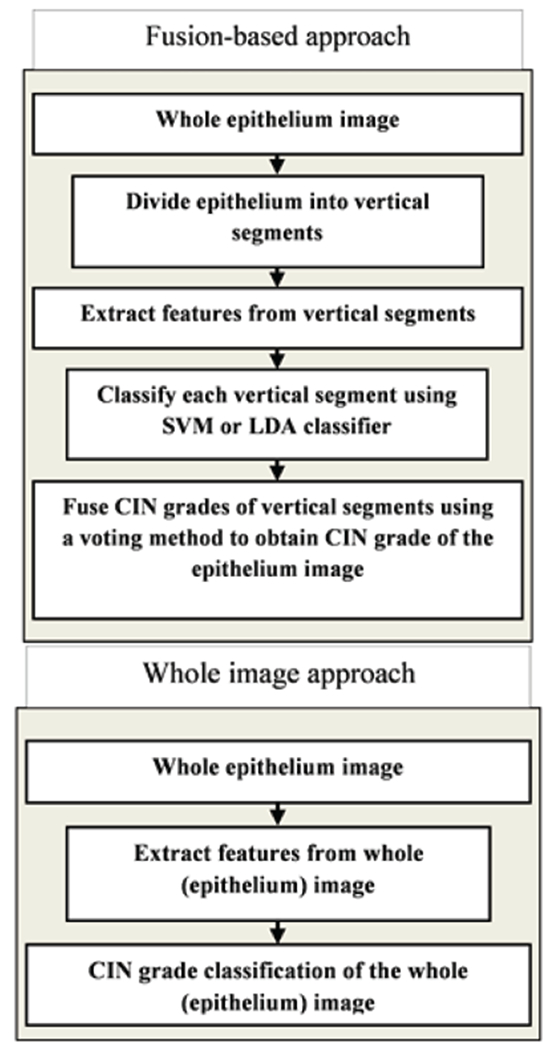
Fusion-based approach vs. whole image approach.
The whole-epithelium image classification in this section is done without generating any of the individual vertical segment images (see Fig. 19 as an example for nuclei feature detection over the whole image). The experiment was investigated to compare the performance of the fusion-based epithelium classification (Section III.A) to the performance obtained by classifying the epithelium image as a whole. Features extracted from the whole image were used as inputs to the SVM/LDA classifier using the same leave-one-image out approach. The same scoring schemes as presented in Section III.A were used to evaluate the performance of the whole epithelium classification. Again, the leave-one-image-out training/testing approach was performed separately for each expert’s CIN labeling of the experimental data set.
Figure 19:

Example image of nuclei detection over whole image without creating vertical segments; the top image is the original epithelium image; bottom is the nuclei mask of this image.
C. Feature Evaluation and Selection
For feature evaluation and selection, a SAS® implementation of Multinomial Logistic Regression (MLR) [24][25][26][27] and a Weka® attribute information gain evaluator were employed. For SAS analysis, MLR is used for modeling nominal outcome variables, where the log odds of the outcomes are modeled as a linear combination of the predictor variables [23][24][25][26]. The p-values obtained from the MLR output are used as a criterion for selecting features with p-values less than an appropriate alpha (α) value [23][24][25][26]. For Weka analysis, the algorithm ranks the features by a parameter called “attributes information gain ratio” where the higher the ratio, the more significant the feature will be for the classification results. For both methods, the automatically generated labels of the vertical segmentations and the feature data are given as input.
IV. Experimental Results and Analysis
A. Experimental Results
We obtained the vertical segment image classifications (CIN grading) using the SVM/LDA classifier with a leave-one-image-out approach based on all the twenty-seven features generated. Then, the vertical segment classifications were fused using a voting scheme to obtain the CIN grade of the epithelium image. We evaluated the performance of these epithelium image classifications using the three approaches presented in section III.A. Table II shows the confusion matrices for the classification results obtained using the fusion-based approach, for the SVM and LDA classifiers, respectively, for both experts (RZ and SF).
Table II.
confusion matrix results for Fusion-based classification using all 27 features (F1-F27) for SVM and LDA classifiers for both experts
| Expert RZ: SVM/LDA | ||||
|---|---|---|---|---|
| Normal (16) | CIN1 (13) | CIN2 (14) | CIN3 (18) | |
| Normal | 14/14 | 0/0 | 0/0 | 0/0 |
| CIN1 | 2/2 | 12/11 | 0/0 | 0/0 |
| CIN2 | 0/0 | 1/1 | 12/14 | 3/3 |
| CIN3 | 0/0 | 0/1 | 2/0 | 15/15 |
| Expert SF: SVM/LDA | ||||
| Normal (14) | CIN1 (14) | CIN2 (17) | CIN3 (16) | |
| Normal | 10/10 | 2/3 | 0/0 | 0/0 |
| CIN1 | 4/3 | 9/9 | 1/1 | 0/0 |
| CIN2 | 0/0 | 3/1 | 16/16 | 1/1 |
| CIN3 | 0/1 | 0/1 | 0/0 | 15/15 |
In the following, we provide summary comments for these Table II results, and compare them with the previous results published in [9], which used the RZ expert CIN labeling of the image set. (1) For the Exact Class Label, we obtained an accuracy of 86.9%/82.0% (RZ/SF) using the SVM classifier and 88.5%/82.0% (RZ/SF) using the LDA classifier, (previous [9]: 62.3% LDA) (2) For the Normal vs. CIN scoring scheme, SVM classifier accuracy was 96.7%/90.2% (RZ/SF) and LDA classifier 96.7%/90.2% (RZ/SF) (previous [9]: 88.5% LDA) (3) For the Off-by-One class scoring scheme, SVM had accuracy of 100%/100% (RZ/SF) and LDA, 98.4%/96.7% (RZ/SF) (previous [9]: 96.7%).
In the order to evaluate the performance of the fusion-based approach for epithelium classification, we also carried out classification using the entire epithelium image. For the whole image classification, we again used the SVM and LDA classifiers. Table III shows the whole image classification results for both experts.
Table III.
Confusion matrix results for whole image classification using all 27 features (f1-f27) for svm and lda classifiers for both experts
| Expert RZ: SVM/LDA | ||||
|---|---|---|---|---|
| Normal (16) | CIN1 (13) | CIN2 (14) | CIN3 (18) | |
| Normal | 15/9 | 0/4 | 0/1 | 0/0 |
| CIN1 | 1/5 | 8/5 | 3/2 | 3/1 |
| CIN2 | 0/1 | 2/3 | 8/8 | 5/8 |
| CIN3 | 0/1 | 3/1 | 3/3 | 10/9 |
| Expert SF: SVM/LDA | ||||
| Normal (14) | CIN1 (14) | CIN2 (17) | CIN3 (16) | |
| Normal | 9/10 | 2/3 | 0/0 | 0/0 |
| CIN1 | 5/3 | 6/8 | 2/3 | 1/1 |
| CIN2 | 0/1 | 5/2 | 11/8 | 7/8 |
| CIN3 | 0/0 | 1/1 | 4/6 | 7/7 |
From Table III, the Exact Class Label scoring scheme provided an accuracy of 67.2%/54.1% (RZ/SF) and 50.8%/54.1% (RZ/SF) using the SVM classifier and LDA classifiers, respectively. The Normal vs. CIN scoring scheme yielded an accuracy of 98.4%/88.6% (RZ/SF) and 80.3%/88.6% (RZ/SF) for the SVM and LDA classifiers, respectively. The Off-by-One scoring scheme obtained an accuracy of 90.2%/96.7% (RZ/SF) and 93.4%/95.1% for the SVM and LDA classifiers, respectively.
The corresponding accuracy figures from previous research [9] for the LDA classifier are given in the following. Exact Class Label scoring: 39.3%; Normal vs. CIN scoring: 78.7%; Off-by-One scoring (called “windowed class” in [9]): 77.0%.
For feature evaluation and selection experiments, all twenty-seven features extracted from the individual vertical segments were used as inputs to the SAS MLR algorithm. We used α=0.05 as the threshold to determine statistically significant features. The overall twenty-seven features with p-values are presented in Table VII (Appendix). From Table VII, features with a p-value smaller than 0.05 are considered statistically significant features.
In addition, all twenty-seven features and the truth labels were used as input for the Weka® information gain evaluation algorithm [27]. The algorithm ranks the features by an “attribute information gain ratio” (AIGR) which ranges from 0 to 1. The larger the ratio is, the more likely that the feature is considered by the algorithm. The twenty-seven features and corresponding AIGR values are shown in Table VII (Appendix).
Based on the statistically significant features shown in Table VII, we selected the feature set consisting of features F1, F3, F4, F5, F7, F9, F10, F12, F13, F14, F15, F18, F21, F22, F23, F24, F26, F27 as the input feature vectors for the fusion-based classification. Note that all these features were selected based on the SAS MLR test of statistical significance except for F23 and F24, which were selected since they have relatively high information gain ratio (AIGR) among the twenty-seven features (the 2nd place and 3rd place in Table VII of Appendix). Our experiment compared classification accuracies using this reduced set of features to the results using entire twenty-seven feature set, and also compared to the classification accuracies obtained in the previous research [9].
The reduced feature classifications were done for the fusion-based method only to remain consistent with the previous research [9]. The classification algorithms (SVM/LDA) were applied to the reduced features, followed by fusing of the vertical segment classifications to obtain the CIN grade of the epithelium. The resulting classifications obtained in this approach are shown as confusion matrices in Table IV for both experts.
Table IV.
Confusion matrix results for fusion-based classification using reduced feature set for SVM and LDA classifiers for both experts
| Expert RZ: SVM/LDA | ||||
|---|---|---|---|---|
| Normal (16) | CIN1 (13) | CIN2 (14) | CIN3 (18) | |
| Normal | 14/14 | 0/0 | 0/0 | 0/0 |
| CIN1 | 2/2 | 10/12 | 0/0 | 0/0 |
| CIN2 | 0/0 | 2/1 | 12/13 | 3/1 |
| CIN3 | 0/0 | 1/0 | 2/1 | 15/17 |
| Expert SF: SVM/LDA | ||||
| Normal (14) | CIN1 (14) | CIN2 (17) | CIN3 (16) | |
| Normal | 11/10 | 3/2 | 0/0 | 0/0 |
| CIN1 | 3/3 | 9/11 | 1/1 | 0/0 |
| CIN2 | 0/1 | 2/1 | 16/16 | 1/1 |
| CIN3 | 0/0 | 0/0 | 0/0 | 15/15 |
From Table IV, the following correct classification rates were obtained for the reduced features using the SVM-based classifier: Exact Class Label classification of 83.6%/83.6% (RZ/SF), Normal vs. CIN classification of 96.7%/90.2% (RZ/SF) and Off-by-One classification of 98.4%/100% (RZ/SF). From Table IV, the correct classification rates using the LDA classifier were obtained as: Exact Class Label classification of 88.5%/85.3% (RZ/SF), Normal vs. CIN classification of 95.1%/90.2% (RZ/SF), and Off-by-One classification of 100%/98.4% (RZ/SF). The highest correct classification rates obtained in previous work using the same experimental data set and leave-one-out training/testing approach with the LDA classifier and are summarized as follows [9]: Exact Class label of 70.5%, Normal vs. CIN of 90.2%, and Off-by-One classification of 100%.
B. Analysis of Results
In this section we use the classification results from Section IV.A, to compare: a) the performance among the scoring approaches, b) the performance between the SVM and LDA classifiers and c) the performance between previous research [9] and this study. Table V gives an overview of the correct recognition rates in different classification schemes examined in this research.
Table V.
CIN discrimination rates for Fusion-based classification using all features, whole image classification and reduced feature set fusion-based classification for both experts
| Fusion-based classification | ||
|---|---|---|
| SVM (RZ/SF) | LDA (RZ/SF) | |
| Exact Class Label | 86.9%/82.0% | 88.5%/82.0% |
| Normal vs. CIN | 96.7%/90.2% | 96.7%/90.2% |
| Off-by-One | 100%/100% | 98.4%/96.7% |
| Whole image classification | ||
| SVM (RZ/SF) | LDA (RZ/SF) | |
| Exact Class Label | 67.2%/54.1% | 50.8%/54.1% |
| Normal vs. CIN | 98.4%/88.6% | 80.3%/88.6% |
| Off-by-One | 90.2%/96.7% | 93.4%/95.1% |
| Reduced feature set | ||
| SVM (RZ/SF) | LDA (RZ/SF) | |
| Exact Class Label | 83.6%/83.6% | 88.5%/85.3% |
| Normal vs. CIN | 96.7%/90.2% | 95.1%/90.2% |
| Off-by-One | 98.4%/100% | 100%/98.4% |
From Table V, the fusion-based classification approach shows improvement (except for same results for Normal vs. CIN) compared to the whole image classification approach, when all the feature vectors are used as input for the classifiers. For the fusion-based vs. whole image classification, the fusion-based approach shows an improvement of 19.7% (minimum improvement from the two experts from 67.2% to 86.9%) for SVM and 27.9% (minimum improvement from the two experts from 54.1% to 82.0%) for LDA using the Exact Class Label scoring scheme. For the Normal vs. CIN scoring scheme, an accuracy improvement of 1.7% (minimum improvement from the two experts from 88.5% to 90.2%) for the LDA classifier, although we note an accuracy decline of 1.7% (from 98.4% to 96.7%) was observed for the SVM classifier. For Off-by-One scoring scheme, classification accuracy increases 3.3% (minimum of two experts from 96.7% to 100%) and 1.6% (minimum of two experts from 95.1% to 96.7%) for SVM and LDA, respectively.
With feature reduction added to fusion-based classification, the fusion-based method improves in half the comparisons. Specifically, the Exact Class Label accuracy for SVM declines by 3.3% (minimum improvement from two experts of 86.9% to 83.6%) and LDA’s accuracy yields zero improvement (minimum from two experts of 88.5% to 88.5%). For Normal vs CIN, there is no improvement (0%) for SVM for both experts, and a 1.6% loss (minimum from two experts of 96.7% to 95.1%) in accuracy for LDA. For Off-by-One, the SVM classifier has a 1.6% decline (minimum of experts from 100% to 98.4%), and LDA has zero improvement (from 98.36% to 98.36%), and LDA has a gain of 1.6% (minimum of experts from 98.4% to 100%).
Among all of classification results obtained by the two different classifiers, the highest come from fusion-based classification. The highest Exact Class Label classification accuracy by the two experts was 88.5%/85.3% (LDA, reduced feature set). In comparison, SVM obtained 83.6%/83.6% by both experts for the reduced feature set. The accuracies for Normal vs CIN and Off-by-One are relatively high for both experts (above 90% for both SVM and LDA classifiers, and for both the full and the reduced feature sets). A summary of the results from this study and from previous research [9] is shown in Table VI below. Note that only the LDA classifier was reported in [9].
Table VI.
Summary of classification accuracies: previous research vs. reduced feature set results in current work.
| Previous work [9] | Current Work (RZ/SF) | |||
|---|---|---|---|---|
| LDA | SVM | LDA | ||
| Fusion based classification | Exact Class Label | 62.3% | 86.9%/82.0% | 88.5%/82.0% |
| Normal vs. CIN | 88.5% | 96.7%/90.2% | 96.7%/90.2% | |
| Off-by-One | 96.7% | 100%/100% | 98.4%/96.7% | |
| Whole image classification | Exact Class Label | 39.3% | 67.2%/54.1% | 50.8%/54.1% |
| Normal vs. CIN | 78.7% | 98.4%/88.5% | 80.3%/88.5% | |
| Off-by-One | 77.0% | 90.2%/96.7% | 93.4%/95.1% | |
| Reduced feature classification | Exact Class Label | 70.5% | 83.6%/83.6% | 88.5%/85.3% |
| Normal vs. CIN | 90.2% | 96.7%/90.2% | 95.1%/90.2% | |
| Off-by-One | 100% | 98.4%/100% | 100%/98.4% | |
In examining the classification results, the majority of the Exact Class Label classification errors are off-by-one CIN grade. This is supported with the high Off-by-One classification rates for the different experiments performed. Fig. 20 shows an example of an image with expert label of CIN2 (RZ) that was labeled as a CIN3 by the LDA classifier.
Fig. 20:
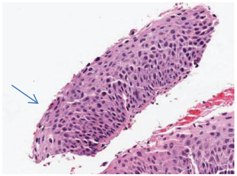
Misclassification example of a CIN2 image labeled as a CIN3.
Inspecting Fig. 20, nuclei bridge across the epithelium and are relatively uniform in density in the lower left-hand portion of the epithelium (see arrow). The nuclei features and layer-bylayer Delaunay triangle features, particularly in the vertical segments containing the lower left-hand portion of the epithelium, provide for a higher CIN grade. In other regions of the epithelium, the nuclei density is not as uniform across the epithelium, which could provide for a less severe CIN grade label for the epithelium.
Fig. 21 shows an example of an image with expert label of CIN3 (RZ) that was labeled as a CIN1 by the LDA classifier. This image has texture, nuclei distribution and color typical of a CIN3 grade. However, the white gaps present along the epithelium were detected as acellular regions, leading to the misclassification.
Fig. 21:
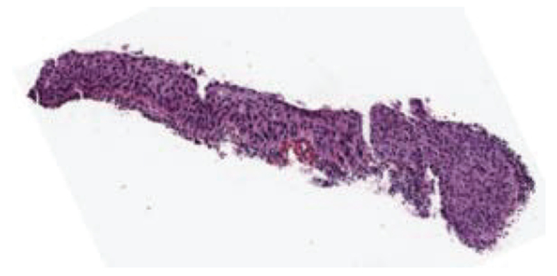
Misclassification example of a CIN3 image labeled as a CIN1.
The overall algorithm was found to be robust in successful identification of nuclei. Nuclei in the two lightest-stained slides and the two darkest-stained slides were counted. An average of 89.2% of nuclei in all four slides was detected. The 89.2% nuclei detection rate observed represents an advance over the results of Veta et al [28], who found 85.5% to 87.5% of nuclei (not strictly comparable, as these results were for breast cancer). The finding of a high percentage of nuclei in the lightest- and darkest-stained slides shows that the algorithm is adaptable and robust with regard to varying staining.
The approach in this study expands the techniques of other researchers who often process but a single cell component: the nucleus. We show in this work that the transition from benign to cancer affects the whole cell. We have shown that not only nuclei, but in fact features of the entire cell, including intercellular spaces, are changed due to the more rapidly growing cells. Thus, one of the top four features by p value is the proportion of regions of cytoplasm in the image (F12).
We also sought to use layers to better represent the CIN transition stages. The number of Delaunay triangles in the middle layer was also one of the top four features by p-value, validating our approach of analysis by layers. The last two features with most significant p-values were the energy of GLCM (sum of squared elements in GLCM in horizontal and vertical directions). The energy in the GLCM appears to capture the growing biological disorder as the CIN grade increases.
We emphasize that, between the previous research [9] and our current work, (1) the training and testing data sets are the same; (2) the classifier (LDA) is the same and we investigated the SVM classifier; and (3) the scoring schemes, (Exact Class Label, Normal vs. CIN, and Off-by-One) are the same (in the previous research, Off-by-One was called “windowed class”). There are two differences between the previous and current work. First, CIN classification results are reported for two experts (RZ and SF) in this study to demonstrate CIN classification improvement over previous work, even with variations in the expert CIN truthing of the experimental data set. Second, three acellular features (F18,F21,F22) and two layer-by-layer triangle (F26,F27) nuclei features were found to be significant (from Table VII), which are new in the current work, contribute to improved CIN discrimination capability over previous work.
For the fusion-based method applied to all the feature vectors, Table VI shows Exact Class Label accuracy increases by 19.7% (from 62.3% to 82.0% for the lower of the two expert results) for LDA. For the whole image method, LDA improved by 14.8% (from 39.3% to 54.1% for the lower of the two expert results). For fusion-based classification with reduced feature vectors, accuracy increases by 14.8% (from 70.5% to 85.3% for the lower of the two experts) for LDA. Since Exact Class Label is the most stringent of the scoring schemes we used, we interpret these results as showing a substantial gain in classification in classification accuracy when using the nuclei features and nuclei-related features.
The Off-by-One classification achieved excellent classification accuracy (100%) with the svM and LDA classifiers, which matches the results from the previous study [9]. This classification metric gives more evidence of the similarity of neighboring classes (Normal/CIN1 or CIN1/CIN2 or CIN2/CIN3) and the difficulties in discriminating between them [6][7][8]. It is also consistent with the intra- and inter-pathologist variation in labeling of these images. The two experts for this study differed in the CIN labeling of five images (out of 61) (or 8.2%) in the experimental data set, with the experts differing by only 1 CIN grade (higher or lower) in each of the five cases.
Overall, the 88.5%/85.3% accuracy by the two experts of Exact Class Label prediction using the reduced features is 23.0% higher than published results for automated CIN diagnosis (62.3%) as presented by Keenan et al. in [12], 17.3% higher than the accuracy of the method used by Guillaud et al. (68%) in [11] and 14.8% higher than the accuracy of the method by De [9], although we note that only in the comparison with De were the same training and testing sets used. The classification results presented in this study for the two experts only differed by greater than 8.2% in the Exact Class Label of the whole image. Thus, the experimental results suggest that the involvement of nuclei and nuclei-related features using vertical segment classification and fusion for obtaining the image-based CIN classification is an improvement over the existing methods for automated CIN diagnosis. Even though our method outperformed published results, we note that there is potential for further improvement.
V. Summary and Future Work
In this study, we developed new features for the automated CIN grade classification of segmented epithelium regions. New features include nuclei ratio features, acellular area features, combination features and layer-by-layer triangle features. We carried out epithelium image classification based on these ground truth sets: 1) two experts labeled sixty-two whole epithelium images as Normal, CIN1, CIN2, and CIN3, and 2) investigator-labeling of 10 vertical segments within each epithelium image into the same four CIN grades. The vertical segments were classified using an SVM or LDA classifier, based on the investigator-labeled training data of the segments with a leave-one-out approach. We used a novel fusion-based epithelium image classification method which incorporates a voting scheme to fuse the vertical segment classifications into a classification of the whole epithelium image. We evaluated the classification results with three scoring schemes, and compared the classification differences by classifiers, by scoring schemes, and the classification results of this research as compared to our previous work [9].
We found that the classification accuracies yielded in this study with nuclei features outperformed that of the previous work [9]. Using the LDA classifier upon the reduced set of features, and based on an Off-by-One classification scoring scheme for epithelium region classification, correct prediction rates as high as 100% were obtained. Normal vs. CIN classification rates were as high as 96.72%, whereas the rates for Exact Class Labels were as high as 88.52% using a reduced set of features. Future research may include use of adaptive critic design methods for classification of CIN grade. Also, it is important to include more cervix histology images to obtain a comprehensive data set for different CIN grades. With the enhancement of the data set, inter- or intrapathologist variations can be incorporated [6].
Gwilym Lodwick, among his many contributions to diagnostic radiology, contributed to our basic knowledge of pattern recognition by both humans and computers. The importance of diagnostic signs, which he also termed minipatterns, was stated: “Signs, the smallest objects in the picture patterns of disease, are of vital importance to the diagnostic process in that they carry the intelligence content or message of the image.” [29] In this context, Professor Lodwick also maintained that these signs are at the heart of the human diagnostic process. The results of our study appear to indicate that the new layer-by-layer and vertical segment nuclei features, in the domain of cervical cancer histopathology, provide useful signs or mini-patterns to facilitate improved diagnostic accuracy. With the advent of advanced image processing techniques, these useful signs may now be employed to increase the accuracy of computer diagnosis of cervical neoplasia, potentially enabling earlier diagnosis for a cancer that continues to exact a significant toll on women worldwide.
Fig. 7:
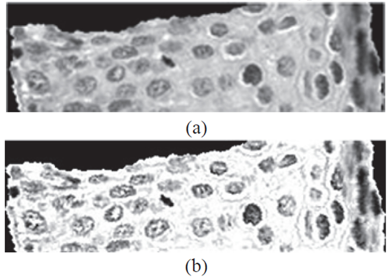
Example of image preprocessing. (a) Original luminance image I. (b) Sharpened image Isharpen obtained after average-filtering of I.
VII. Acknowledgements
This research was supported [in part] by the Intramural Research Program of the National Institutes of Health (NIH), National Library of Medicine (NLM), and Lister Hill National Center for Biomedical Communications (LHNCBC). In addition we gratefully acknowledge the medical expertise and collaboration of Dr. Mark Schiffman and Dr. Nicolas Wentzensen, both of the National Cancer Institute’s Division of Cancer Epidemiology and Genetics (DCEG).
This research was supported, in part, by the Intramural Research Program of the National Institutes of Health (NIH), National Library of Medicine (NLM), and Lister Hill National Center for Biomedical Communications (LHNCBC).
VI. Appendix
Table VII.
Features with corresponding p-values and AIGR (attributes information gain ratio)
| Feature | p –value | AIGR |
|---|---|---|
| F1 | 0.0013 | 0.226 |
| F2 | >0.05 | 0.21 |
| F3 | 0.0182 | 0.026 |
| F4 | 0.0425 | 0.204 |
| F5 | 0.0604 | 0.171 |
| F6 | >0.05 | 0.0309 |
| F7 | 0.0051 | 0.2057 |
| F8 | >0.05 | 0.079 |
| F9 | 0.0001 | 0.080 |
| F10 | 0.0001 | 0.034 |
| F11 | >0.05 | 0.205 |
| F12 | 0.0001 | 0.169 |
| F13 | 0.0033 | 0.2287 |
| F14 | 0.0037 | 0.1800 |
| F15 | 0.1101 | 0.505 |
| F16 | >0.05 | 0.2713 |
| F17 | >0.05 | 0.2897 |
| F18 | 0.0201 | 0.2357 |
| F19 | >0.05 | 0.2717 |
| F20 | >0.05 | 0.2990 |
| F21 | 0.0320 | 0.3608 |
| F22 | 0.0646 | 0.3295 |
| F23 | >0.05 | 0.3975 |
| F24 | >0.05 | 0.4713 |
| F25 | >0.05 | 0.1001 |
| F26 | 0.0001 | 0.1037 |
| F27 | 0.0001 | 0.2644 |
Contributor Information
Peng Guo, The Department of Electrical and Computer Engineering of Missouri University of Science and Technology in Rolla, MO 65409-0040, USA (pgp49@mst.edu).
Koyel Banerjee, The Department of Electrical and Computer Engineering of Missouri University of Science and Technology in Rolla, MO 65409-0040 (kbnm6@mst.edu).
R. Joe Stanley, Department of Electrical and Computer Engineering of Missouri University of Science and Technology in Rolla, MO 65409-0040 USA (stanleyj@mst.edu).
Rodney Long, Lister Hill National Center for Biomedical Communications for National Library of Medicine, National Institutes of Health, DHHS in Bethesda, MD 20894, USA (long@nlm.nih.gov).
Sameer Antani, Lister Hill National Center for Biomedical Communications for National Library of Medicine, National Institutes of Health, DHHS in Bethesda, MD 20894, USA.
George Thoma, Lister Hill National Center for Biomedical Communications National Library of Medicine, National Institutes of Health, DHHS in Bethesda, MD 20894, USA.
Rosemary Zuna, Department of Pathology for the University of Oklahoma Health Sciences Center in Oklahoma City, OK 73117, USA.
Shellaine R. Frazier, Surgical Pathology Department for the University of Missouri Hospitals and Clinics in Columbia, MO 65202, USA
Randy H. Moss, Department of Electrical and Computer Engineering of Missouri University of Science and Technology in Rolla, MO 65409-0040 USA (rhm@mst.edu).
William V. Stoecker, Stoecker & Associates, Rolla MO, 65401, USA (wvs@mst.edu)
References
- [1].World Health Organization, Department of Reproductive Health and Research and Department of Chronic Diseases and Health Promotion Comprehensive Cervical Cancer Control: a Guide to Essential Practice, 2nd ed. Geneva, Switzerland: WHO Press, p. 7, 2006. [Google Scholar]
- [2].Jeronimo J, Schiffman M, Long LR, Neve L and Antani S, “A tool for collection of region based data from uterine cervix images for correlation of visual and clinical variables related to cervical neoplasia,” Proc. 17th IEEE Symp. Computer-Based Medical Systems: IEEE Computer Society, 2004, pp. 558–62. [Google Scholar]
- [3].Kumar V, Abba A, Fausto N and Aster J, “The female genital tract,” in Robbins & Cotran Pathologic Basis of Disease, 9th ed., Kumar V, Abbas AK, Aster JC Eds., Philadelphia: Saunders, 2014, ch. 22, pp 1017–1021. [Google Scholar]
- [4].He L, Long LR, Antani S and Thoma GR, “Computer assisted diagnosis in histopathology,” in Sequence and Genome Analysis: Methods and Applications, Zhao Z, ed., iConcept Press, Hong Kong, ch. 15, pp. 271–287, 2011. [Google Scholar]
- [5].Wang Y, Crookes D, Eldin OS, Wang S, Hamilton P and Diamond J, “Assisted diagnosis of cervical intraepithelial neoplasia (CIN),” IEEE J. Selected Topics in Signal Proc., vol.3, no.1, pp.112–121, 2009. [Google Scholar]
- [6].McCluggage WG, Walsh MY, Thornton CM, Hamilton PW, Date A, Caughley LM and Bharucha H, “Inter- and intra-observer variation in the histopathological reporting of cervical squamous intraepithelial lesions using a modified Bethesda grading system,” BJOG: An Int. J. Obstet. and Gynecol, vol. 105, no. 2, pp. 206–210, 1988. [DOI] [PubMed] [Google Scholar]
- [7].Ismail SM, Colclough AB, Dinnen JS, Eakins D, Evans DM, Gradwell E, O’Sullivan JP, Summerell JM and Newcombe R, “Reporting cervical intra-epithelial neoplasia (CIN): Intra- and interpathologist variation and factors associated with disagreement.” Histopathology, vol. 16, no. 4, pp. 371–376, 1990. [DOI] [PubMed] [Google Scholar]
- [8].Molloy C, Dunton C , Edmonds P, Cunnane MF and Jenkins T, “Evaluation of colposcopically directed cervical biopsies yielding a histologic diagnosis of CIN 1, 2.” J. Lower Genital Tract Dis, vol. 6, pp. 80–83, 2002. [DOI] [PubMed] [Google Scholar]
- [9].De S, Stanley RJ, Lu C, Long R, Antani S, Thoma G, Zuna R, “A fusion-based approach for uterine cervical cancer histology image classification, Comp. Med. Imag. Graph., vol. 37, pp. 475–487, 2013. [DOI] [PMC free article] [PubMed] [Google Scholar]
- [10].Marel JVD, Quint WGV, Schiffman M, van-de-Sandt MM, Zuna RE, Terence-Dunn S, Smith K, Mathews CA, Gold MA, Walker J, Wentzensen N, “Molecular mapping of high-grade cervical intraepithelial neoplasia shows etiological dominance of HPV16,” Int. J. Cancer, vol. 131, pp. E946–E953 (doi: 10.1002/ijc.27532), 2012. [DOI] [PMC free article] [PubMed] [Google Scholar]
- [11].Guillaud M, Adler-Storthz K, Malpica A, Staerkel G, Matisic J, Niekirk DV, Cox D, Poulin N, Follen M, MacAulay C, “Subvisual chromatin changes in cervical epithelium measured by texture image analysis and correlated with HPV,” Gyn. Oncology, vol. 99, pp. S16–23. 2006. [DOI] [PubMed] [Google Scholar]
- [12].Keenan SJ, Diamond J, McCluggage WG, Bharucha H, Thompson D, Bartels PH and Hamilton PW, “An automated machine vision system for the histological grading of cervical intraepithelial neoplasia (CIN),” J. Pathology, vol. 192, no. 3, pp. 351–362, 2000. [DOI] [PubMed] [Google Scholar]
- [13].Maurer CR, Rensheng Q and Raghavan V, “A linear time algorithm for computing exact Euclidean distance transforms of binary images in arbitrary dimensions,” IEEE Trans. Pattern Analysis Mach. Intell, vol. 25, pp. 265–270, Feb. 2003. [Google Scholar]
- [14].Rao CR, Toutenburg H, Fieger A, et al. , Heumann C, Nittner T and Scheid S, Linear Models: Least Squares and Alternatives. Springer Series in Statistics, New York, NY: Springer-Verlag, 1999. [Google Scholar]
- [15].Banerjee K, “Uterine cervical cancer histology image feature extraction and classification,” M.S. Thesis, Dept. Elec. Comput. Eng., MO Univ. S&T., Rolla MO, 2014. [Google Scholar]
- [16].Mathworks, available at: http://www.mathworks.com/help/images/ref/regionprops.html.
- [17].Gonzalez R and Woods R. Digital Image Processing, 2nd ed. Englewood Cliffs, NJ: Prentice-Hall, 2002. [Google Scholar]
- [18].Borovicka J, “Circle detection using Hough transforms.” Course Project: COMS30121-Image Processing and Computer Vision, http://linux.fjfi.cvut.cz/pinus/bristol/imageproc/hw1/report.pdf 2003.
- [19].Preparata FR and Shamos MI. Computational Geometry: An Introduction. New York: Springer-Verlag, 1985. [Google Scholar]
- [20].Krzanowski WJ, Principles of Multivariate Analysis: A User’s Perspective. New York: Oxford University Press, 1988. [Google Scholar]
- [21].Fan RE, Chen PH and Lin CJ. “Working set selection using second order information for training SVM,” J. Mach. Learning Res, vol. 6, pp. 1889–1918, 2005. [Google Scholar]
- [22].Chang CC and Lin CJ. “LIBSVM : a library for support vector machines,” ACM Trans. Intelligent Sys. Tech, vol. 2, no. 27, pp. 1–27, 2011. [Google Scholar]
- [23].Agresti A, An Introduction to Categorical Data Analysis. New York, NY: John Wiley & Sons, 1996. [Google Scholar]
- [24].Pal M, “Multinomial logistic regression-based feature selection for hyperspectral data,” Int. J. Appl. Earth Observation Geoinformation, vol. 14, no. 1, pp. 214–220, 2012. [Google Scholar]
- [25].Li T, Zhu S and Ogihara M, “Using discriminant analysis for multiclass classification: an experimental investigation,” Knowl. Inf. Syst, vol. 14, no. 4, pp. 453–472, 2006. [Google Scholar]
- [26].Hosmer D and Lemeshow S, (2000), Applied Logistic Regression, 2nd. ed. New York: John Wiley & Sons, 2000. [Google Scholar]
- [27].Hall M, Frank E, Holmes G, Pfahringer B, Reutemann P and Witten IH, “The WEKA Data Mining Software: An Update,” SIGKDD Explorations, vol. 11, no. 1, pp. 10–18, 2009. [Google Scholar]
- [28].Veta M van Diest PJ, Kornegoor R, Huisman A, Viergever MA, Pluim JPW, “Automatic Nuclei segmentation in h&e stained breast cancer histopathology images,” PLoS ONE, vol. 8, no. 7, p. e70221 (doi: 10.1371/journal.pone.0070221), 2013. [DOI] [PMC free article] [PubMed] [Google Scholar]
- [29].Lodwick G, “Diagnostic signs and minipatterns,” Proc Ann. Symp. Comput. Appl. Med. Care, vol. 3, pp. 1849–1850, 1980. [Google Scholar]


