Surrogate minimal depth as an importance measure for variables in random forests

Abstract

Motivation

It has been shown that the machine learning approach random forest can be successfully applied to omics data, such as gene expression data, for classification or regression and to select variables that are important for prediction. However, the complex relationships between predictor variables, in particular between causal predictor variables, make the interpretation of currently applied variable selection techniques difficult.

Results

Here we propose a new variable selection approach called surrogate minimal depth (SMD) that incorporates surrogate variables into the concept of minimal depth (MD) variable importance. Applying SMD, we show that simulated correlation patterns can be reconstructed and that the increased consideration of variable relationships improves variable selection. When compared with existing state-of-the-art methods and MD, SMD has higher empirical power to identify causal variables while the resulting variable lists are equally stable. In conclusion, SMD is a promising approach to get more insight into the complex interplay of predictor variables and outcome in a high-dimensional data setting.

Availability and implementation

https://github.com/StephanSeifert/SurrogateMinimalDepth.

Supplementary information

Supplementary data are available at Bioinformatics online.

1 Introduction

In the last years, the investigation of different types of omics data, measuring e.g. gene expression, methylation status or metabolite concentrations has become popular to characterize patients and healthy controls, to understand complex diseases and to develop effective treatments (Ibrahim et al., 2016). Since omics datasets are large and heterogeneous, statistical and computational analysis poses several challenges: First, the big p and small n problem results from the situation that the number of variables is much bigger than the number of probands that are investigated (Johnstone and Titterington, 2009). Second, the variables usually have complex relationships, due to underlying molecular networks and pathways that should be incorporated into the analysis. Third, the vast majority of the variables are usually not relevant for the research subject, which means that the extensive dataset could be reduced to a smaller set of important variables.

It has been shown that machine learning methods, and in particular random forests (RFs) (Breiman, 2001), can be successfully applied to exploit omics data for classification, regression (Strobl et al., 2009) and survival outcomes (Ishwaran et al., 2011). One main goal of these applications, besides the generation of valid prediction models, is variable selection, i.e. the separation of relevant from irrelevant variables. RFs provide a permutation variable importance (VIMP) that is obtained by permuting the variables and calculating the difference in prediction error. Hence, variables are ranked according to their impact on prediction performance. Various approaches have been developed to select important variables based on VIMP and were recently evaluated in a comprehensive comparison study (Degenhardt et al., 2017). However, VIMP is influenced by specific variable characteristics (Strobl et al., 2007) and the correlation structure of the variables (Nicodemus et al., 2010). As a result, conditional variable importance has been introduced which uses a modified permutation scheme that preserves the correlation structure between predictor variables (Strobl et al., 2008). The computational requirements, however, prohibits an application to high-dimensional data. Because VIMP is rather difficult to study in detail (Ishwaran, 2007) we strive for an approach that is independent of prediction errors. Ishwaran et al. (2010) developed a method called minimal depth (MD) that simply determines variable importance by the position of the variables in the decision trees and thus, is only based on the decision tree structures. Since trees should be adequately deep to obtain reliable results, this method is especially susceptible to the big p and small n problem. Furthermore, the correlation structure of the variables is not considered in this approach. Hence, we propose a new variable selection technique that is based on decision tree structures that includes variable relations, and that is feasible for high-dimensional datasets with low numbers of observations.

To compensate for missing values in the data, Breiman (Breiman et al., 1984) developed the concept of surrogate variables. This means that for every node in the tree additional splits of other variables are determined that are capable to replace the original splits as good as possible when the primary variables are missing. In this article, we show that surrogate variables can also be used for other purposes. First, we will demonstrate that the relationship between a primary split variable and a surrogate variable are a proxy for the relation between the variables. Since the relationship between primary and surrogate variable takes into account the association with the outcome, it goes beyond the analysis of pairwise correlations and will consequently be called relation in this article. Subsequently we will introduce a new approach incorporating surrogate variables into the concept of MD called surrogate minimal depth (SMD).

2 Materials and methods

2.1 RF variable selection

RF is a machine-learning approach that uses a large number of individual binary decision trees based on different bootstrap samples of the training data. At each node, the optimal split separating observations in below (daughter node 1) and above (daughter node 2) the split point is identified from a set of randomly chosen candidate predictor variables. Hence, the split that is stored for each node consists of a split variable and an optimized split point. To predict the outcome variable a majority vote over all trees is taken. Besides providing accurate classification and regression of observations, RF analyses are conducted to identify variables important for prediction. In a recent comparison study of several variable selection methods, the Boruta (Kursa et al., 2010) and the Vita approach (Janitza et al., 2018) demonstrated the best performance (Degenhardt et al., 2017). Both methods are based on the permutation importance (VIMP), which is calculated as the difference of prediction performance before and after permuting the values of the variable averaged over all trees. The Boruta approach selects predictor variables whose importance is significantly larger than those of permuted versions of itself. The Vita method calculates P-values based on an empirical null distribution using only non-positive importance scores.

2.2 Identification of surrogate variables

The concept of surrogate splits was developed by Breiman et al. (1984) to compensate for missing values in datasets when RF is applied. In addition to the best split of a specific node (called primary split), several additional splits are stored. They are based on other predictor variables than the one used in the primary split and result in a similar assignment of observations to the child nodes as the primary split. For a specific node surrogate variables and their split points are determined by the two daughter nodes of the primary split. For each predictor variable the agreement n_surr between surrogate split q and primary split p is calculated as the number of observations that are assigned to the same daughter nodes. The adjusted agreement agree(p, q) (also see https://cran.r-project.org/web/packages/rpart/vignettes/longintro.pdf) is then defined as

$$\mathrm{agree}\left(p,\mathrm{ }q\right)=\mathrm{ }\frac{n_{\mathrm{surr}}-\mathrm{ }{n}_{\mathrm{maj}}\mathrm{ }}{n_{\mathrm{total}}-\mathrm{ }{n}_{\mathrm{maj}}},$$ (1)

where n_total denotes the total number of observations at the respective node and n_maj the number of observations that are assigned to the same daughter nodes when the majority rule is applied, i.e. all observations are assigned to the daughter node with the larger number of observations.

An adjusted agreement value of 1 means an exact agreement of the surrogate split to the primary split, i.e. the same observations are assigned to the right and left daughter nodes, respectively. A value of 0 corresponds to the performance of the majority rule. A negative value of adjusted agreement means that the surrogate split assigns fewer observations in accordance with the primary split than the majority rule. At each non-terminal node in the tree, adjusted agreement between the primary split and the split of all other predictor variables with optimized split points (according to similarity to the primary split) is calculated. Subsequently the s surrogate splits with the largest positive adjusted agreement are stored for each of these nodes. Note that it may happen that less than s potential surrogate splits outperform the majority rule. In this case less than s surrogate splits are used for this node so that the average number of surrogate variables in a specific level j of the trees, denoted as$\mathrm{ }\overline{s_j}$, or across the whole forest, denoted as $\overline{s}$, might be smaller than the predefined value of s. In our simulation studies, we systematically vary the parameter s to evaluate its influence on the selection of important variables and on the recovery of known correlation patterns between predictor variables.

2.3 Exploiting surrogate variables to investigate variable relations

One of the goals of this study is to assess whether surrogate variables can be exploited to identify relationship patterns in the data. In order to achieve this goal a new relation parameter that is determined from the decision trees of RFs will be introduced in this section. To analyze the relation of predictor variable B to predictor variable A, all nodes where the primary split variable is variable A and variable B is included in the set of surrogate variable are considered. The set of these nodes will be called nodes(A, B). The total adjusted agreement agree_A, B is then defined as the sum of the adjusted agreements for all these nodes:

$${\mathrm{agree}}_{A,B}={\sum }_{i=1}^{\left|\mathrm{nodes}\left(A,B\right)\right|}\mathrm{agree}\left(p_i^A,\mathrm{ }{q}_i^B\right),$$ (2)

where $p_i^A\mathrm{ }$and $q_i^B\mathrm{ }$denote the primary split based on variable A and the surrogate split based on variable B for node i. The relation between the variables A and B is then defined as the mean adjusted agreement m_AB which is determined by dividing the total adjusted agreement by nodes(A), the total number of nodes based on primary variable A:

$$m_{\mathit{AB}}=\frac{{\mathrm{agree}}_{A,B}}{\left|\mathrm{nodes}\right(A\left)\right|}.$$ (3)

Note that the mean adjusted agreement is not symmetric in contrast to a correlation coefficient or similarities based on distance metrics. A relation between predictor variables A and B is considered relevant if the corresponding mean adjusted agreement is larger than a threshold T_S. The calculation of T_S, takes into account the average number of surrogate variables per split $\overline{s}$ the total number of variables in the dataset p, and the average adjusted agreement agree_m and is weighted by a user defined factor t > 1:

$$T_s=\mathrm{ }\frac{\mathrm{ }\overline{s}}{p}·{\mathrm{agree}}_m·t.$$ (4)

The average adjusted agreement agree_m is calculated as the average of the adjusted agreements between all primary splits and surrogate variables in each node of each tree in the forest (see Supplementary Formula S1).

We used the values 1, 5, 10, 20 and 100 for t. Larger values can be employed to focus on the strongest relations between predictor variables while low values can be applied to also include weaker relations.

2.4 SMD variable importance

MD of variable A is defined as the average level of the first split based on variable A across all trees with at least one split based on variable A (Ishwaran et al., 2010). In contrast to variable selection methods that are based on VIMP, important variables have low MD values. The threshold T_MD to separate relevant from non-relevant variables is determined by the average MD of non-relevant variables in a setting where the outcome is independent of all predictor variables. It is calculated by the sum over all levels of the product of level j, the probability that a variable is chosen by chance π_j at level j and the number of nodes n_j that are present in level j:

$$T_{\mathrm{MD}}=\sum _{j}j\mathrm{ }{\pi }_j\mathrm{ }{n}_j.$$ (5)

The idea of our new variable selection approach SMD is to apply the importance measure of MD defined by the first appearance not only to primary split variables but also to the occurrence of surrogate variables. Hence, the importance measure of variable B is defined as the level of the first split where B is either the primary split variable or a surrogate variable for any other variable. Since an increasing number of surrogate variables will decrease SMD variable importance values for all variables and particularly for causal, correlated variables, the threshold T_SMD to identify important variable has to be adapted: The number of nodes n_j on level j is increased by the respective average number of surrogate variables of the respective layer $\overline{s_j}$:

$$T_{\mathrm{SMD}}=\sum _{j}j\mathrm{ }{\pi }_j\mathrm{ }(n_j+\overline{s_j}).$$ (6)

2.5 Implementation and analyses

We utilized the R package ranger (Wright and Ziegler, 2017) for our investigation and implemented MD variable importance from the R package randomForestSRC and the determination of surrogate variables from the R package rpart in the ranger environment. Our new R package SurrogateMinimalDepth is available at https://github.com/StephanSeifert/SurrogateMinimalDepth. For every RF we generated 10 000 trees. To investigate variable relations with surrogate variables and the variable importance with MD and SMD we used an mtry value of p^(3/4) as recommended in (Ishwaran et al., 2011) and a minimal node size of 1. The parameters s (see Section 2.2) for SMD of simulated data and t (see Section 2.3) for experimental data was varied with ∼0.5, 1, 2, 5 and 10% of the total number of predictor variables, and 1, 5, 10, 20 and 100, respectively. As default parameters for Boruta and Vita variable importance we used the same parameters as in (Degenhardt et al., 2017), namely mtry of $\sqrt{p}$ and a P-value of 0.01 and mtry of p/3 and p.t of 0, respectively. The minimal node size was set to 1 for both methods. In order to examine the influence of the parameters mtry, and p.t and P-value on the variable selection results of Vita and Boruta, additional analyses were conducted. All combinations of mtry values of p^(3/4) and 0.33*p, and p.t values of 0.01 and 0.05 for Vita, and mtry values of p^(3/4) and sqrt(p) and P-values of 0.001 and 0.02 for Boruta were used for this comparison.

For the run time investigation, a computer with 2 × Intel(R) Xeon(R) CPU E5-2620 v4 @ 2.10 GHz, 16 cores (32 threads) and 64 GB DDR4 RAM was used.

2.6 Data

2.6.1 Simulation study 1

The first simulation study was conducted to evaluate surrogate variables for the investigation of variable relations and to compare SMD to MD for variable selection. A quantitative outcome was simulated based on six so called relevant basic variables X₁,…, X₆ according to the following linear model:

$$\mathrm{Y}={\mathrm{X}}_1+{\mathrm{X}}_2+{\mathrm{X}}_3+{\mathrm{X}}_4+{\mathrm{X}}_5+{\mathrm{X}}_6+\epsilon .$$

Each of the relevant basic variables was sampled independently from a standard normal distribution X_i ∼ N(0, 1), i = 1, …, 6. The noise followed a N(0, 0.2) distribution. We further simulated three additional basic variables X₇, X₈, X₉, which are independent of Y and of X₁ to X₆ and hence will be called non-relevant. Furthermore, variables correlated to the three relevant basic variables X₁, X₂, X₃ and to the three non-relevant basic variables X₇, X₈ and X₉ were generated. For each of those 6 basic variables X_i, 10 correlated variables (denoted as cX_i = cX_i⁽¹⁾, …, cX_i⁽¹⁰⁾) were obtained by the simulateModule function of the R package WGCNA (Langfelder and Horvath, 2008) using strong correlation (correlation coefficient of 0.9) for X₁ and X₇, moderate correlation (0.6) for X₂ and X₈, and low correlation (0.3) for X₃ and X₉. Additional independent predictor variables [non-correlated variables (ncV)] were simulated using the standard normal distribution to reach a total number of 1000 variables. In the following, we will denote the predictor variables X₁, X₂, X₃, X₄, X₅ and X₆ as well as cX₁–cX₃ as relevant variables and the other variables as non-relevant variables. A graphical summary of the simulation scenario is shown in Supplementary Figure S1.

We simulated the outcome Y for a population of 100 independent individuals and generated 50 replicates for this population. For the evaluation surrogate variables were analyzed as described in Section 2.3 and variable selection using MD (see Ishwaran et al., 2010) and SMD (see Section 2.4) was applied.

In order to investigate type I error rates of SMD in a binary setting, as e.g. in a case-control scenario we also simulated a scenario with 1000 independent N(0, 1) predictor variables and a binary outcome which was simulated independently of any of the predictor variables. A total of 50 replicates for 50 cases and 50 controls were simulated and SMD was applied (see Section 2.4). Type I error rates for the null scenario were estimated as the number of variables selected by SMD divided by the total number of predictor variables.

2.6.2 Simulation study 2

In order to compare SMD to state-of-the-art methods under realistic correlation structures the second simulation study was conducted. A similar classification model as in (Degenhardt et al., 2017) was used and gene expression data were simulated using the R package Umpire (Zhang et al., 2012). Gene expression values for cases and controls were generated using a multivariate normal distribution for a 12 592-dimensional random vector with a mean vector of zeroes. The covariance matrix was obtained from an experimental RNA-microarray dataset of breast cancer patients containing 12 592 genes (see Section 2.6.3) similar as in (Janitza et al., 2018). The set of effect sizes was set to {−2, −1, −0.5, 0.5, 1, 2} and for each effect size 25 variables out of the 12 592 variables were randomly chosen resulting in 150 causal variables. To associate these causal variables with the outcome, the means of these causal variables were modified according to the corresponding effect size in the case individuals. The other non-chosen variables and the covariance matrix are the same for cases and controls. For each set of 150 causal variables, we simulated two datasets of 200 individuals (100 controls and 100 cases) and repeated this process 50 times including the random selection of the 150 causal variables.

We estimated the evaluation criteria stability, classification error, empirical power, sensitivity and false positive rate (FPR) to compare the different variable importance approaches SMD, MD, Boruta and Vita.

Stability was determined using the Jaccard’s index (He and Yu, 2010) of the two sets of selected variables from the two respective datasets. This index is defined as the ratio of the length of the intersection and the length of the union of the two sets of variables. It is 1 if the two sets are identical and 0 if they do not have any variable in common. For the determination of the classification error, each of the two datasets of each replicate was used to select variables, on which a RF model (ntree = 10 000, mtry = 4197, nodesize = 20) was trained (training set) while the other dataset was used as validation set. Subsequently, the mean classification error for each pair was calculated and reported. Empirical power of causal variables was determined separately for each absolute effect size by the fraction of correct selections among all replicates. Sensitivity was obtained by dividing the number of correctly selected causal variables by the total number of causal variables. In order to determine the FPR the set of null variables was defined for each replicate separately since different variables were simulated as causal. Because variables at least moderately correlated to causal variables are usually of interest in association studies as well, only variables that were non-causal and that were uncorrelated to each of the causal variables (Pearson’s correlation coefficient < 0.2) were included in the set of null variables used for the FPR. The FPR was calculated by dividing the number of selected null variables by the total number of null variables.

2.6.3 Experimental dataset

For the investigation of experimental data, we used two breast cancer gene expression datasets from two different technologies [next generation sequencing (NGS)-based and microarray] for the prediction of estrogen receptor status that were obtained from The Cancer Genome Atlas (Network CGA, 2012). Please refer to (Degenhardt et al., 2017) for details about the data and data pre-processing.

The variable selection methods SMD (with 100 surrogate variables), Boruta and Vita were compared using the parameters classification error and stability. Similar as in simulation study 2 for each of the variable selection approaches each of the two datasets was used once to select variables and to train a RF (ntree = 10 000, mtry = 4197, nodesize = 51) and once as validation set to estimate classification error. The mean error of both validation datasets is reported in the following. Because of the technological differences of the datasets a modified version of the Jaccard’s index using the minimum number of selected genes as denominator was utilized to evaluate stability of the variable selection method (also see Degenhardt et al., 2017). In addition, surrogate variables were used to identify variables that are related to the gene ESR1 (estrogen Receptor 1) and the results were compared with a list of correlated genes that was obtained from a published study on estrogen receptor status in breast cancer patients (Andres and Wittliff, 2012).

3 Results

3.1 Variable relations and first application of SMD (simulation study 1)

In order to assess whether surrogate variables can be exploited to investigate variable relations, the mean adjusted agreement between each basic variable and all other variables as well as between the first variable of each group and all other variables was determined (see Supplementary Figs S2 and S3). Based on the respective mean adjusted agreement and the calculated threshold, related variables for each basic variable as well as for the first variable of each group of relevant and non-relevant, correlated predictor variables were selected. Figure 1 shows the selection frequencies of the three variables that were most often selected for each of the considered predictor variables. For the relevant basic variables X₁ to X₃ (Fig. 1A) the respective correlated variables (cX₁ to cX₃) are most commonly selected. However, the frequency depends on the predefined correlations: The variables featuring high and medium correlation values of 0.9 and 0.6 to the basic variables X₁ and X₂, respectively, are always selected while the variables having a low correlation of 0.3 to variable X₃ are only selected in ∼30% of the replicates.

Fig. 1.

Selection frequencies across the 50 replicates in simulation study 1 to investigate variable relations based on surrogate variables for the basic variables (A) and the first variable of the groups of relevant as well as the non-relevant, correlated predictor variables (B). The number of surrogate variables was set to 100 and related variables were selected by comparison to a threshold T_s with t = 5. For each variable, the three most often selected variables are shown and the different groups were summarized in one plot. The bars of the correlated variables are colored in gray

Interestingly, a similar result is achieved for the non-relevant correlated basic variables X₇–X₉: The variables of cX₇ and cX₈ featuring high and medium correlations are always selected for the basic variables X₇ and X₈, respectively. The variables of cX₉, however, are again selected as surrogate for variable X₉ in only ∼30% of the replicates. The relevant non-correlated basic variables X₄–X₆ show very low selection frequencies for all variables and groups.

The selection frequencies for the respective first variable of the correlated groups are also showing an equivalent behavior between relevant correlated (cX₁–cX₃) and non-relevant correlated (cX₇–cX₉) variables: For the variables with high correlations (cX₁ and cX₇) the respective basic variables (X₁ and X₇) and groups (cX₁ and cX₇) are always selected, while for the variables with medium correlations (cX₂ and cX₈) only the respective basic variables (X₂ and X₈) are always selected and the respective groups (cX₂ and cX₈) are selected in only ∼60% of the replicates. For the variables featuring low correlations (cX₃ and cX₉) only the respective basic variables (X₃ and X₉) are selected in ∼40% of the cases.

In summary, surrogate variables can be exploited to identify high, medium and to some degree even low correlations between variables. As a matter of fact correlations between non-relevant variables can also be examined when a sufficient number of trees (in this case 10 000) are built and the number of relevant variables is relatively small.

Figure 2A and B shows the results for MD and SMD variable importance using a predefined number of surrogates (s) of 100. The relevant basic variables X₂–X₆ show a MD variable importance that is below the threshold for the vast majority of the replicates. Hence, those variables are selected in most cases. X₁, the relevant basic variable of the group with the highest correlation of 0.9 (cX₁) is only selected in less than half of the replicates. This can be explained by the fact that the variables from the group cX₁ are likely to replace X₁ in the decision trees leading to higher MD values for X₁ compared with the values for relevant basic variables without correlated groups (X₄, X₅ and X₆). This fact is also supported by the lower MD values of group cX₁ compared with the non-relevant variables (X₇, X₈, X₉ and ncV). The other predictor variables and variable groups mostly have MD values above the threshold and, thus, are not selected by MD in most replicates. The reason for this rather poor performance of MD can be attributed to the big p small n problem, since using 1000 instead of 100 observations shows a higher correspondence to the simulation setup (see Supplementary Fig. S4)

Fig. 2.

MD (A) and SMD (B) using 100 surrogate variables. Boxplots of MD and SMD for 50 replicates and the respective thresholds (dashed lines) to select important variables are shown. The six groups of correlated variables (cX₁–cX₃ and cX₇–cX₉) as well as the ncVs are summarized in one boxplot

The results of SMD variable importance, however, show values below the threshold for the basic variables X₁–X₆ and the group cX₁ for almost all replicates and for the group cX₂ for most of the replicates. Hence, SMD has a higher chance of selecting the causal basic variables and also variables that are highly correlated to these variables than MD. With this method an opposite effect of the presence of correlated variables compared with MD can be observed: Basic variable X₁ features lower SMD values than the variables X₄, X₅ and X₆. Here, choosing correlated variables from the group cX₁ instead of X₁ in the tree building process doesn’t result in lower minimal depth values for X₁, since X₁ is always chosen as surrogate in those cases (see Fig. 1). However, the probability that X₁ or any variable of the group cX₁ is chosen as candidate split variable is substantially higher than the probability that an uncorrelated basic variable X₄, X₅ or X₆ is chosen.

In order to investigate the influence of the predefined number of surrogate splits on SMD, variable selection based on SMD was conducted with numbers ranging from zero to 100 (Supplementary Fig. S5 shows the results for SMD with s = 5, 10, 20 and 50). Figure 3 compares the selection frequency of the various types of predictor variables across the different numbers. Using zero surrogates (red dots) is equivalent to MD variable importance, resulting in relatively low selection frequencies of 50–80% for the relevant basic variables (X₁–X₆) and below 30 and 20% for the groups featuring high (cX₁) and medium (cX₂) correlations to the respective basic variables. When five surrogate variables are used for SMD, (green triangles in Fig. 3) the relevant basic variables (X₁–X₆) and the relevant group featuring high correlations (cX₁) are selected for most of the replicates. However, the non-relevant correlated basic variables X₇ and X₈ show high selection frequencies and the non-relevant group with high correlations (cX₇) shows increased selection frequencies, as well. Similar results are obtained for SMD using 10 surrogate variables (black squares in Fig. 3): All of the relevant basic variables (X₁–X₆) and the group of highly correlated variables (cX₁) are selected in almost all cases, just like non-relevant basic variables (X₇ and X₈) and the group of non-relevant highly correlated variables (cX₇). Probably, non-relevant, correlated variables are selected, since those variables are always used as surrogates when a correlated variable is randomly chosen for the primary split in the tree building process (see Fig. 1). This results in sufficiently low SMD values even though these variables are not chosen more frequently for primary splits than other non-relevant variables.

Fig. 3.

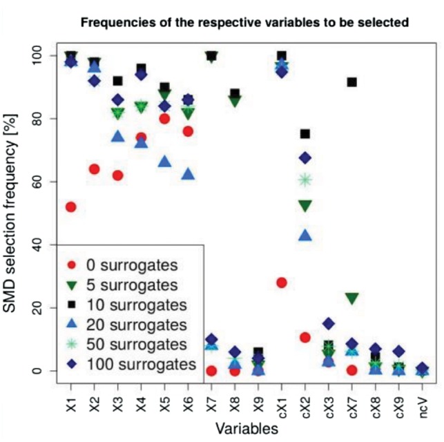
SMD selection frequencies using different numbers of surrogates. For the basic variables each symbol denotes the frequency across all 50 replicates whereas for the six groups of correlated variables (cX₁–cX₃ and cX₇–cX₉) as well as the ncVs the average frequency across all variables in the group is shown

Interestingly, the selection of non-relevant basic variables with high and medium correlation (X₇ and X₈) does not happen on a significant scale when 20 surrogate variables are used for SMD (blue triangles in Fig. 3). In this case the threshold, that is lower than in the SMD investigation with less surrogate variables, is low enough to exclude these variables. However, the non-relevant and non-correlated variables (X₄–X₆) are selected in only 60–80% of the replicates, and thus even more infrequently than in MD variable selection (red dots). Thus, the threshold in this scenario is so low that relevant non-correlated variables can be rejected, only because they are rarely selected as surrogate variables for other relevant variables.

When the number of surrogates is increased to 50 all of the relevant basic variables (X₁–X₆) and the highly correlated group cX₁ are selected in >80% of the replicates and the medium correlated group cX₂ still is selected in ∼60% of the cases. In addition to this, the non-relevant basic variables (X₇–X₉) and groups (cX₇–cX₉) are usually rejected. Hence, using more surrogate variables than the simulation scenario suggests, leads to more accurate results, since correlated non-relevant variables are rejected more frequently and relevant non-correlated variables are selected more often.

Using 100 surrogate variables instead of 50 slightly increases the selection frequencies for almost all variables, including relevant variables (X₁–X₆) and groups (cX₁–cX₃), as well as non-relevant, correlated variables (X₇–X₉) and groups (cX₇–cX₉).

The additionally conducted null scenario analysis also shows that slightly more non-causal variables are selected when higher numbers of surrogates for SMD are used. Although no variable is selected in any replicate when SMD is applied with 5, 10 and 20 surrogates, the type 1 error rate is 0.00004 and 0.00036 when SMD is applied with 50 and 100 surrogates, respectively.

In summary, using relatively low numbers of surrogate variables can result in decreased rejection of correlated non-relevant variables and increased rejection of non-correlated relevant variables. When sufficiently high numbers of surrogate variables are chosen; however, the true relevance of the variables can be reproduced adequately by SMD variable selection: The basic variables, as well as the variables with high and partially even the variables with medium correlation are frequently selected.

3.2 Comparison of SMD to state-of-the-art methods (simulation study 2)

Figure 4 summarizes the results for the second simulation study that was performed to compare SMD with different numbers of surrogate variables to state-of-the-art methods under realistic correlation structures. Figure 4A displays the two evaluation criteria classification error and stability. An optimal method would be located in the upper left corner, i.e. would have a large stability and a small classification error. Figure 4B shows empirical power stratified by effect size. Similar to the first simulation study, MD (red dots in Fig. 4) performs weakly in this simulation scenario: The empirical power of causal variables with all effect sizes is very low and the stability is zero meaning that different small sets of variables are selected for the two datasets that were simulated using the same causal variables. Hence, the classification error of this method is crucially bigger than the errors of the other methods that achieve a perfect classification. SMD with 50 surrogate variables (green triangle in Fig. 4) shows high empirical power for causal variables with effects sizes of |1| and |2| as well as a high stability of over 80%. Even though comparatively few surrogate variables are used, both empirical power and stability are higher than the respective values that were obtained by the Vita method (purple cross in Fig. 4).

Fig. 4.

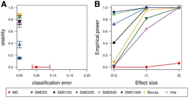
Comparison of the performance of SMD using different numbers of surrogates with MD, Boruta and Vita in simulation study 2. Median, as well as the interquartile range over all 50 replicates for stability and classification error (A) and median frequencies of the empirical power for the different effect sizes (B) are shown

The results using a larger number of 100 surrogate variables for SMD show a substantially higher empirical power for low effect sizes (|0.5|) of ∼40%, while the stability remains high at around 80%. Hence, the empirical power is substantially higher than for the Boruta method (orange stars in Fig. 4).

Raising the number of surrogate variables to 200 (blue triangles in Fig. 4) shows interesting differences to the application of SMD with fewer surrogate variables: The empirical power of causal variables with low effect sizes rises to around 70%, but the stability decreases to ∼40%. This trend continues when SMD with 500 and 1000 surrogates (green square crosses and blue diamonds in Fig. 4) is applied with empirical power of around 90% for causal variables with low effect sizes and stability values of <20%.

The average number of selected variables is 3.5 for MD, 85 for Vita, 91 for SMD50, 108 for Boruta, 127 for SMD100, 240 for SMD200, 779 for SMD500 and 1337 for SMD1000. It is obvious that using higher numbers of surrogate variables results in the selection of higher numbers of variables. Among those variables, however, also increasing numbers of wrongly selected variables are present, which is obvious from the FPR that is presented in Supplementary Figure S6.

Supplementary Figure S7 shows the results of the analyses of simulation study 2 applying Vita and Boruta with the same value for mtry that was used for SMD and MD and various values for the method specific parameters p.t (Vita) and P-value (Boruta). It is obvious that similar results are obtained when mtry and P-value (for Boruta) are changed, while higher values for p.t (for Vita) result in higher sensitivities, but also much higher FPRs. Based on these results it can be concluded that using the same parameter values [mtry = sqrt(p) and P-value = 0.01 for Boruta and mtry = 0.33 P and p.t. = 0 for Vita in Supplementary Fig. S7] as in (Degenhardt et al., 2017) is appropriate for the comparison with SMD.

In summary, using low numbers of surrogate variables for SMD leads to stable results that have a similar or even higher power than state-of-the-art methods. When higher numbers are applied, the lists of selected variables are more diverse, inter alia because different variables that are not correlated to causal variables are chosen in each of the two datasets in each replicate.

3.3 Application to experimental datasets

Figure 5 displays the analysis results of the experimental datasets. Since the true causal variables are not known only classification error and the stability of the variable selection were used for the variable selection performance comparison (Fig. 5A). The classification errors of the three methods are similar and range from 0.0737 for SMD to 0.708 for Boruta. As in (Degenhardt et al., 2017) a different definition of stability using the minimum number instead of the union of selected variables was used to compensate for the different characteristics of the datasets. SMD variable selection features a much higher stability of 80.9% than Boruta (48.5%) and Vita (27%) (Supplementary Fig. S8 shows the stability values using the original definition). SMD selected 393 and 1448 genes in the NGS and microarray datasets. The numbers are 130 and 111 for Vita, and 529 and 476 for Boruta.

Fig. 5.

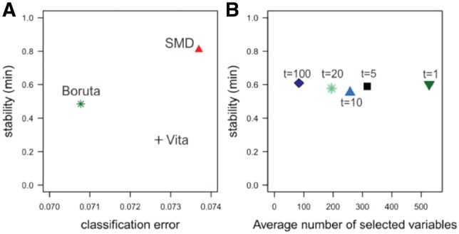
Performance comparison based on experimental datasets for SMD using 100 surrogate variables, Boruta and Vita (A) as well as performance comparison to identify variables related to ESR1 utilizing different thresholds (B). Stability and classification error for the two datasets are shown in (A). In (B), the stability and the average number of variables related to ESR1 using SMD with different thresholds T_s based on different values for the parameter t (see Formula 2) is displayed. Note that a different definition of stability defined relative to the minimum and not the union of the two sets of selected variables is used

The average run time for SMD was ∼1.5 h and thus faster than the run time of Boruta (∼2 h) and slower than the run time of Vita (∼5 min).

For the identification of related variables the selection process explained in Section 2.3 was performed for the gene ESR1 that is known to encode the estrogen receptor-alpha. In Figure 5B, the performance comparison using different thresholds T_s based on different values for the parameter t is displayed. Utilizing higher values for the threshold and, thus, stricter requirements for the selection, results in the consideration of lower numbers of variables related to ESR1. Hence, only ∼84 related variables are identified when t = 100 is utilized (blue diamond in Fig. 5B), while ∼528 variables are defined as related when a threshold with t = 1 is used (green triangle in Fig. 5B). The stability, however, is very similar at ∼60% when different thresholds are applied. This indicates that the parameter t can be adjusted to either focus on strongly related variables only or to include also moderately related variables without increasing the number of wrongly selected variables. Information about mean adjusted agreement between ESR1 and genes identified as related for each threshold value for the NGS and microarray datasets can be found in the Supplementary Tables.

In order to assess these lists, we analyzed the presence and position of 11 genes with Pearson correlation coefficients of >0.6 to ESR1 that were taken from a study examining breast cancer patients (Andres and Wittliff, 2012). Table 1 shows that all of these genes are present in the list based on the microarray data and nine of the eleven genes are in the list of the NGS data. Most of the variables feature comparatively high values for mean adjusted agreement, so that they are also selected when the respective highest threshold is utilized (ranks labeled with a in Table 1). However, the relation that is represented by the mean adjusted agreement goes beyond the analysis of pairwise correlations since it also includes information about the causality of the variables. The correlation coefficient is, nevertheless, an important influence on the variable relation analyzed by surrogate variables. Hence, selection of related variables shows results that are in accordance to known variable correlations (Table 1) and variables with high correlation coefficients also feature high mean adjusted agreement values (Supplementary Fig. S9).

Table 1.

Evaluation of genes that are strongly correlated with ESR1 (Pearson’s correlation coefficient > 0.6)

Gene	Correlationa	Rank (NGS)	Rank (microarray)
GATA3	0.85	3b	9b
XBP1	0.82	20b	42b
SCUBE2	0.79	34b	28b
NAT1	0.75	88c	32b
EVL	0.74	—	71b
RabeP1	0.74	26b	300d
SLC39A6	0.73	12b	60b
TCEAL1	0.69	37b	114c
PGR	0.69	50b	145c
TBC1D9	0.65	2b	2b
TPBG	0.61	—	310d

^aPearson’s correlation coefficient according to (Andres and Wittliff, 2012).

^b,c,dGenes selected utilizing thresholds of t = 100, 20 and 5, respectively.

4 Discussion and conclusion

In this study, we introduced new possibilities to exploit surrogate variables in RFs besides the already established application to compensate for missing values in the data (Breiman, 2001).

In the first approach, we showed that the mean adjusted agreement of surrogate variables can serve as proxy to investigate variable relations. We demonstrated this in a simulation study where correlation patterns could be reproduced by the analysis of mean adjusted agreement. The correlation coefficient, however, is only one influence on this relation that is also strongly affected by the mutual causality of the respective variables. Hence, this new relation parameter is very promising to analyze variables in complex effect interactions and to identify relevant pathways and networks underlying complex diseases.

In the second approach, we utilized surrogate variables to improve MD variable importance and presented a new variable selection method, SMD. Since MD reveals a ‘ceiling effect’ meaning that trees cannot be grown deep enough for reliable variable selection this method is particularly affected by the big p and small n problem (Ishwaran et al., 2010). Including surrogate variables to calculate minimal depth values, however, strongly increases the number of variables that are considered in every node. Hence, the big p and small n problem is not as detrimental when SMD is applied and considerably higher amounts of causal and relevant variables are selected in the simulation studies. However, the optimal number of surrogates for SMD strongly dependents on the variable relations and the number of truly relevant variables. Hence, further applications to experimental and simulated data are needed for a comprehensive overview but we tentatively recommend using ∼ 1% of the total variables as utilized number of surrogate variables for future applications.

In this article, we applied SMD to the classification and regression of gene expression data. Since SMD is using the tree structures for the evaluation, the application to survival data is also possible, as it has been demonstrated by the application of MD (Ishwaran et al., 2010). Furthermore, RFs do not make any assumptions about the predictor variables or the outcome, which means that omics data with different distributions, such as categorical data (genotypes) or proportional data (methylation) could also be analyzed by SMD. However, in the current version of the R package only the analysis of continuous data is possible, which will be changed in a future update.

The focus of this study was on variable selection in high dimensional omics data; however, RF analysis and variable selection is also successfully applied on low-dimensional datasets with many more observations than predictor variables. In this situation, it might not be necessary to include surrogate variables in the variable selection step since MD variable selection often leads to similar results (data not shown). However, the SMD approach can be used to better understand the relations between important predictor variables.

The comparison of SMD to state-of-the-art variable selection methods showed that SMD displays a more complete picture of the variables that are involved, since a much higher fraction of all relevant variables are identified. The average run time of SMD is between the methods that were used for comparison making it a well applicable method for variable selection.

SMD variable importance, just as Gini importance (Strobl et al., 2007), is biased in favor of variables with many possible split points such as categorical variables with a large number of categories or quantitative variables (data not shown). Therefore, our study used only quantitative predictor variables. Recently, a modified version of the Gini importance called Actual Impurity Reduction has been proposed which is unbiased regarding the number of categories and minor allele frequency (Nembrini et al., 2018). This approach could be combined with the concept of surrogate variables to allow the analysis of variables of different types.

In conclusion, exploiting surrogate variables is very promising for powerful variable selection and for investigating the complex interplay of predictor variables and outcome variables in high-dimensional omics datasets.

References

- Andres A., Wittliff J. (2012) Co-expression of genes with estrogen receptor-α and progesterone receptor in human breast carcinoma tissue. Horm. Mol. Biol. Clin. Investig., 12, 377.. [DOI] [PubMed] [Google Scholar]
- Breiman L. et al. (1984) Classification and Regression Trees, Chapman & Hall/CRC Press, London/Boca Raton, pp. 140–150. [Google Scholar]
- Breiman L. (2001) Random forests. Mach. Learn., 45, 5–32. [Google Scholar]
- Degenhardt F. et al. (2017) Evaluation of variable selection methods for random forests and omics data sets. Brief. Bioinform., 16.10.2017, doi: 10.1093/bib/bbx124. [DOI] [PMC free article] [PubMed] [Google Scholar]
- He Z., Yu W. (2010) Stable feature selection for biomarker discovery. Comput. Biol. Chem., 34, 215–225. [DOI] [PubMed] [Google Scholar]
- Ibrahim R. et al. (2016) Omics for personalized medicine: defining the current we swim in. Expert Rev. Mol. Diagn., 16, 719–722. [DOI] [PubMed] [Google Scholar]
- Ishwaran H. (2007) Variable importance in binary regression trees and forests. Electron. J. Stat., 1, 519–537. [Google Scholar]
- Ishwaran H. et al. (2010) High-dimensional variable selection for survival data. J. Am. Stat. Assoc., 105, 205–217. [Google Scholar]
- Ishwaran H. et al. (2011) Random survival forests for high-dimensional data. Stat. Anal. Data Min., 4, 115–132. [Google Scholar]
- Janitza S. et al. (2018) A computationally fast variable importance test for random forests for high-dimensional data. Adv. Data Anal Classif, 4, 885–915. [Google Scholar]
- Johnstone I.M., Titterington D.M. (2009) Statistical challenges of high-dimensional data. Philos. Trans. Royal Soc. A, 367, 4237–4253. [DOI] [PMC free article] [PubMed] [Google Scholar]
- Kursa M.B. et al. (2010) Feature selection with the Boruta package. J. Stat Softw., 36, 1–13. [Google Scholar]
- Langfelder P., Horvath S. (2008) WGCNA: an R package for weighted correlation network analysis. BMC Bioinformatics, 9, 559.. [DOI] [PMC free article] [PubMed] [Google Scholar]
- Nembrini S. et al. (2018) The revival of the Gini importance? Bioinformatics, doi: 10.1093/bioinformatics/bty373. [DOI] [PMC free article] [PubMed] [Google Scholar]
- Network C.G.A. (2012) Comprehensive molecular portraits of human breast tumours. Nature, 490, 61.. [DOI] [PMC free article] [PubMed] [Google Scholar]
- Nicodemus K.K. et al. (2010) The behaviour of random forest permutation-based variable importance measures under predictor correlation. BMC Bioinformatics, 11, 110.. [DOI] [PMC free article] [PubMed] [Google Scholar]
- Strobl C. et al. (2007) Bias in random forest variable importance measures: illustrations, sources and a solution. BMC Bioinformatics, 8, 1.. [DOI] [PMC free article] [PubMed] [Google Scholar]
- Strobl C. et al. (2008) Conditional variable importance for random forests. BMC Bioinformatics, 9, 307.. [DOI] [PMC free article] [PubMed] [Google Scholar]
- Strobl C. et al. (2009) An introduction to recursive partitioning: rationale, application, and characteristics of classification and regression trees, bagging, and random forests. Psychol. Methods, 14, 323–348. [DOI] [PMC free article] [PubMed] [Google Scholar]
- Wright M.N., Ziegler A. (2017) ranger: A Fast Implementation of Random forests for high dimensional data in C++ and R. J Stat Softw, 77, 1–17. [Google Scholar]
- Zhang J. et al. (2012) Simulating gene expression data to estimate sample size for class and biomarker discovery. Int. J. Adv. Life Sci., 4, 44–51. [Google Scholar]
Associated Data
This section collects any data citations, data availability statements, or supplementary materials included in this article.