Synaptic Heterogeneity and Stimulus-Induced Modulation of Depression in Central Synapses

Abstract

Short-term plasticity is a pervasive feature of synapses. Synapses exhibit many forms of plasticity operating over a range of time scales. We develop an optimization method that allows rapid characterization of synapses with multiple time scales of facilitation and depression. Investigation of paired neurons that are postsynaptic to the same identified interneuron in the buccal ganglion of Aplysiareveals that the responses of the two neurons differ in the magnitude of synaptic depression. Also, for single neurons, prolonged stimulation of the presynaptic neuron causes stimulus-induced increases in the early phase of synaptic depression. These observations can be described by a model that incorporates two availability factors, e.g., depletable vesicle pools or desensitizing receptor populations, with different time courses of recovery, and a single facilitation component. This model accurately predicts the responses to novel stimuli. The source of synaptic heterogeneity is identified with variations in the relative sizes of the two availability factors, and the stimulus-induced decrement in the early synaptic response is explained by a slowing of the recovery rate of one of the availability factors. The synaptic heterogeneity and stimulus-induced modifications in synaptic depression observed here emphasize that synaptic efficacy depends on both the individual properties of synapses and their past history.

A principle site of information transfer in the nervous system is the synapse between two neurons. The synapse is not a passive, static conduit. Rather, it depends on its past history and may change on a spike-by-spike basis (Byrne, 1982; Dittman and Regehr, 1998; Stevens and Wesseling, 1998; Gomis et al., 1999;Neves and Lagnado, 1999). Consequently, mathematical modeling techniques are increasingly used to help unravel the complexity of the synapse (Zengel and Magleby, 1982). The necessity of using these techniques arises because a large number of mechanisms act in concert (Zucker, 1989). Moreover, the relative importance of each mechanism can change with the statistical properties of the input spike train, such as frequency and patterning (Wiersma and Adams, 1950; Gillary and Kennedy, 1969; Wachtel and Kandel, 1971;Brezina et al., 2000a). Modeling approaches can be used, for example, to quantify and localize the effects of modulators (Cleland and Selverston, 1997; Jorge-Rivera et al., 1998); to quantify how synapses change with development (Hill and Jin, 1998); to understand neuromuscular control (Brezina et al., 2000a); to elucidate the role of synaptic dynamics in cortical gain control (Abbott et al., 1997), computation (Chance et al., 1998), and network synchrony (Abarbanel et al., 1996; Neiman et al., 1999; Bressloff, 1999; Tsodyks et al., 2000); and to develop rapid, computer-based methods for screening pharmacological compounds.

An important step in synaptic modeling was the application of random spike trains to collect data (Krausz and Friesen, 1977). Appropriately chosen random stimulus trains contain intervals at all time scales, and thus the relevant processes need not be identified a priori. The Volterra method is a powerful technique that has traditionally been used to analyze data collected with random spike trains (Ogura, 1972; Krausz, 1975;Krausz and Friesen, 1977). However, the disadvantages of this method are that it is difficult to collect sufficient data and difficult to interpret the results (Hung et al., 1977; Berger et al., 1988; Sclabassi et al., 1988).

To address these difficulties, Sen et al. (1996)introduced “synaptic decoding.” Optimization techniques are used to fit models based on synaptic physiology to data collected with random spike trains. Although this model has worked well in a neuromuscular junction, it cannot describe synapses with depletion and hence has limited applicability for the study of central synapses (Sen et al., 1996; Chance et al., 1998; Dittman and Regehr, 1998).

Here we extend the Sen et al. (1996) model to synapses with multiple availability factors, using their optimization methodology. The term “availability factor” describes a synaptic component that decrements with each action potential, recovers with a characteristic time course, and scales the response multiplicatively. This generic term can encompass a depletable vesicle pool or a desensitizing population of receptors. The extension was required because we observed that the synaptic responses of central neurons ofAplysia could not be adequately described by synaptic models that lacked multiple availability factors.

The simultaneous IPSC responses of Aplysia neurons postsynaptic to buccal interneuron B4/5 (Gardner, 1990) are described by a synaptic model that incorporated two availability factors: one rapidly recovering and the other slowly recovering (hereafter referred to as the rapid and slow factors). The observation that two neurons respond differently to stimulation of B4/5 is explained by differences in the magnitudes of the rapid and slow factors. We also observed in single neurons that prolonged stimulation of B4/5 increases synaptic depression in subsequent stimuli. These changes are explained by an activity-dependent slowing of the recovery of the rapid factor. Our results are consistent with the physiology of acetylcholine receptor desensitization in Aplysia. This suggests that the available factor model, closely related to the classic depletion model (Abbott et al., 1997;O'Donovan and Rinzel, 1997; Markram et al., 1998), may be successfully applied to receptor desensitization.

MATERIALS AND METHODS

Aplysia electrophysiology. Aplysia care and dissection were performed as described in Church and Lloyd (1994). The ganglion was constantly perfused with artificial seawater with high divalent cations; perfusion solution concentrations were (in mm): 286 NaCl, 165 MgCl₂, 10 KCl, 33 CaCl₂, and 5 NaHCO₃. The high divalent solution raises the threshold for neural firing and is required to quiet intrinsic network activity while allowing for the investigation of specific synapses (Gardner, 1986, 1990). Because the high calcium may influence synaptic dynamics, we do not know whether the observations discussed below would be seen in an intact animal in normal physiological saline.

Recordings of the two postsynaptic neurons were made in two-electrode voltage-clamp mode with two AxoClamp 2B amplifiers (Axon Instruments, Foster City, CA) with electrode resistances ≈4 MΩ and a holding potential of −50 mV. The electrodes were filled with 3 mK-acetate, 30 mm KCl, and 0.1% Fast Green. The presynaptic interneuron B4/5 was stimulated to fire action potentials with 8–10 msec step current pulses of 100–250 nA using a Getting Model 5A microelectrode amplifier (Getting Instruments, San Diego, CA) in current-clamp mode. B4/5 can mediate pure inhibitory, pure excitatory, or diphasic inhibitory/excitatory conductances depending on the follower cell (Gardner and Kandel, 1977). We restricted our investigations to pure inhibitory follower cells [identified as B3, B6, B8, or B9 in Gardner and Kandel (1977)].

Data were low-pass filtered at 1 kHz with a Frequency Devices 902 low-pass filter (Frequency Devices, Haverhill, MA) and digitally sampled at 2 kHz. All recording and stimulation protocols were automated using an AD2210 A/D board (Real Time Devices, State College, PA) interfaced with a personal computer controlled by custom software (Hunter et al., 1998). We present data from a total of seven neurons in three animals. The n = 46 stimulus trains used here had lengths of 2–10 min, mean frequencies of 2–10 Hz, and an exponential, a uniform, or a Gaussian distribution of intervals.

Availability model. The model described below is motivated by the model presented in Sen et al. (1996). In the model presented there, the amplitude of the i -th event is given by an arbitrary nonlinear transformation of an underlying factor, i.e., R(t_i) = F(x(t_i)) where x is an unspecified underlying component and F is the nonlinear transformation. Because x is governed by a linear convolution kernel, for example, a sum of exponential functions with possibly different signs, this model is quite general despite its notational simplicity and can describe systems with multiple time scales of facilitation and depression. However, as Sen et al. (1996) note, this formalism does not encompass the case in which the response is governed by an availability factor, such as a depletable pool of vesicles. We apply the Sen optimization methodology to an extended model that incorporates multiple availability factors.

Our approach is mechanism independent so we use generic terminology: “underlying component,” “available factor,” “fraction activated,” and “response,” and we leave the biological correlates unspecified. Depending on the system, the underlying component could be identified with presynaptic calcium accumulation, the available factor with the store of readily releasable pool of vesicles, the fraction activated with the fraction of available vesicles released, and the response with presynaptic membrane capacitance. Alternatively, the components could be identified with postsynaptic mechanisms, in which the underlying component is neurotransmitter concentration in the synaptic cleft, the available factor is a population of desensitizing receptors, the fraction activated is the fraction of free receptors activated, and the response is postsynaptic current.

Each incoming action potential arrives at time t_i and stimulates an underlying component, x(t_i). The underlying component sums linearly according to a kernel K_x(t), which governs its decay between action potentials:

$$x(t_{\text{i}})=\sum _{{\text{t}}_{\text{j}}\le {\text{t}}_{\text{i}}} K_{\text{x}}(t_{\text{i}}-t_{\text{j}}).$$ Equation 1

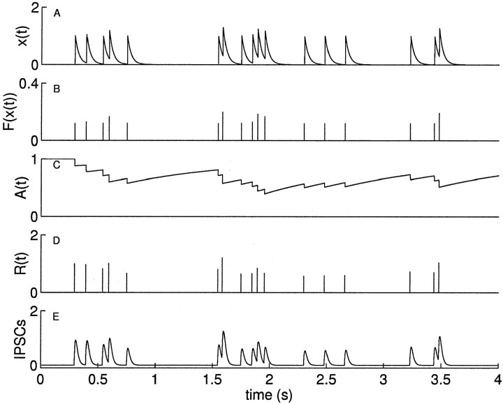
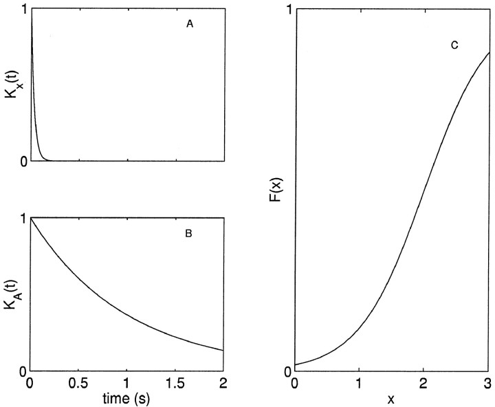
Figure 1A shows the time course of x(t) when K_x, shown in Figure 2A, is an exponential function.

Fig. 1.

Simulation of the available factor model determining IPSC response. A, Each incoming action potential stimulates an underlying factor x, which decays with an exponential time course and sums linearly. B, x at the time of each action potential determines the activated fraction F of the available factor, given by a Boltzmann function of x. C, Availability 𝒜 is decremented by the amount activated and recovers with an exponential time course. D, Response R is proportional amount activated, indicated by thedownward steps in C. E, IPSCs are given by the linear convolution of R with the postsynaptic response kernel.

Fig. 2.

Example model functions. Plots of the functions used in the simulation in Figure 1. A, Decay of x is determined by a single exponential rate constant, K_x(Δ) = exp(−αΔ); α = 50 s⁻¹. B, The recovery of the depleted factor is determined by a single exponential rate constant, K_A(Δ) = exp(−αΔ) where Δ is the time since the last action potential; α = 1 s⁻¹. C, Fraction released is given by a Boltzmann function of x, F(x) = 1/(1 + exp(−α (x − x_1/2))) with x_1/2 = 2 and α = 2.

The underlying component at time t_i determines the fraction, F(x(t_i)), of the available factor that is activated. Figure 1B shows the fraction activated as a function of time. In all of our investigations, we examined monotone F, i.e., the fraction that is activated is an increasing function of the underlying component. A possible choice of F is the properly scaled Boltzmann or Hill function (Fig.2C). For the models of our data, however, the distribution of the underlying component was narrow, and thus we could make the approximation F(x) = αx. This simplifies the model and reduces the number of parameters needed to describe the data.

Availability is decremented at each spike t_i by the amount activated, and between spikes it recovers with a time course given by a function K_A(t). Availability is a discontinuous function of time, with step changes at the time of each action potential, as shown in Figure 1C. We use the notation A⁻(t_i) to indicate the time limit approached from the left and A⁺(t_i) for the limit from the right, which is the fraction available immediately after a spike. Between spikes, availability recovers continuously according to:

$$A^{-}(t)=1-K_A(t-t_{\text{i}})(1-A^{+}(t_{\text{i}}))t_{\text{i}}<t\le t_{\text{i}+1}.$$ Equation 2

K_A(t) has a maximum of 1, which occurs at t = 0, and a minimum of 0, which occurs at t = ∞. At each time t_i, the available factor will decrease by F(x(t_i)) A⁻(t_i), giving the relation:

$$A^{+}(t_{\text{i}})=A^{-}(t_{\text{i}})-F(x(t_{\text{i}}))A^{-}(t_{\text{i}}).$$ Equation 3

Using Equation 3, we can rewrite Equation 2 as:

$$\mathcal{A}(t_{\text{i}+1})=1-K_A(t_{\text{i}+1}-t_{\text{i}})(1-\mathcal{A}(t_{\text{i}})(1-F(x(t_{\text{i}})))),$$ Equation 4

where 𝒜 ≡ A⁻. For the example shown in Figure 1C, K_A is an exponential function (Fig. 2B).

The response R(t_i) is proportional to the product of F and A⁻(t_i):

$$R(t_{\text{i}})=\text{sF}(x(t_{\text{i}}))A^{-}(t_{\text{i}}),$$ Equation 5

where s is a scalar. The response, which is defined for discrete points in time, is shown in Figure 1D; to obtain the full continuous time response shown in Figure 1E, the discrete time response must be convolved with the impulse response kernel as discussed below.

The multiplicative relationship between F and 𝒜 is analogous to the finding that mean quantal content m is given by the product of the probability of release p and the number of quanta N in the quantal analysis ofCastillo and Katz (1954) and is an essential feature of depletion models (Liley and North, 1953; Magleby and Zengel, 1982; O'Donovan and Rinzel, 1997;Varela et al., 1997; Dittman and Regehr, 1998).

Nonetheless, the formulation of the available factor model in Equation5 may be inadequate to describe many synapses, because the dynamics may be determined by multiple, largely independent factors. In the case where N factors sum linearly, the single factor model is extended in a straightforward way with:

$$R(t_{\text{i}})=\sum _{\text{j}=1}^N R_{\text{j}}(t_{\text{i}})=\sum _{\text{j}=1}^N s_{\text{j}}{F}_{\text{j}}(x(t_{\text{i}})){\mathcal{A}}_{\text{j}}(t_{\text{i}}).$$ Equation 6

Because the factors evolve independently, the availability of the j -th factor obeys:

$${\mathcal{A}}_{\text{j}}(t_{\text{i}+1})=1-K_{A_{\text{j}}}(t_{\text{i}+1}-t_{\text{i}})(1-{\mathcal{A}}_{\text{j}}(t_{\text{i}})(1-F_{\text{j}}(x(t_{\text{i}})))).$$

In our experiments, we observed for a given neuron that the magnitude of the first IPSC response was approximately constant between stimuli (see Results). Therefore, for some of our investigations, we normalized the data so that the magnitude of the first IPSC was 1 and imposed the constraint R(t₁) = 1 with the restriction on the last scalar s_N. For the additive factors model given in Equation 6, this restriction is:

$$s_N=\left(1-\sum _{\text{j}=1}^{N-1} R_{\text{j}}(t_1)\right)/(F_N(x(t_1)){\mathcal{A}}_N(t_1)).$$ Equation 7

This constraint reduces the number of parameters by one.

Alternatively, the factors may combine multiplicatively. For example,Magleby and Zengel (1982) found a multiplicative relationship between augmentation and facilitation at the frog neuromuscular junction, although they found an additive relationship between the two components of facilitation. Varela et al. (1997) found that a model with two depression factors that enter multiplicatively described the EPSCs in neocortical slices. In such cases, the multiple factor model may be written as:

$$R(t_{\text{i}})=\prod _{\text{j}=1}^N R_{\text{j}}(t_{\text{i}}),$$ Equation 8

with the first amplitude normalization:

It is also straightforward to extend the model to nonindependent factors, so that the underlying component governing one availability factor (e.g., neurotransmitter concentration in the cleft governing a population of desensitizing receptors) is the response R of a multiple factor model (e.g., presynaptic calcium concentration governing multiple pools of vesicles).

Fitting the model to data. A number of steps are required to fit the model to the data: (1) measure the impulse kernel K of the postsynaptic neuron, (2) extract the magnitudes a_i of the IPSCs from the postsynaptic current record, and (3) use a gradient descent method to optimize fit between the model and the data. The impulse kernel K is simply the average IPSC resulting from a single presynaptic action potential. Gradient descent is a general method of minimizing a function with derivatives that are known (Fletcher, 1987); in this case the error of a model prediction is minimized over the model parameters. By first extracting the magnitudes of the IPSCs rather than working with the entire current record, we were able to reduce the computation time by two to three orders of magnitude for a 30 sec spike train.

A fundamental assumption of this modeling approach is that the measured current response I(t) can be represented as a convolution of δ inputs of amplitudes a_i with a fixed impulse response kernel K. That is:

$$I(t)=\sum _{\text{i}} a_{\text{i}}K(t-t_{\text{i}}),$$ Equation 10

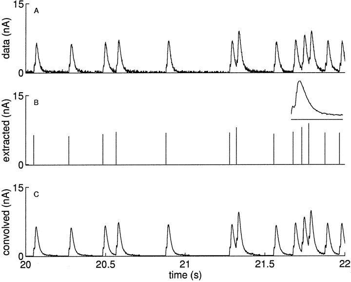
where the index i ranges over the action potentials at times t_i ≤ t. We plot a sample current I(t) in Figure3A. The extracted amplitudes a_i are shown as sticks in Figure 3B, with the time-averaged kernel K shown as an insetin that panel.

Fig. 3.

Extraction of the IPSC amplitudes. A, The IPSCs recorded in a postsynaptic neuron in response to stimulating the presynaptic interneuron B4/5 with a 5 Hz exponentially distributed train of impulses. We show a segment out of the middle of the recording from 20–22 sec. B, We extract the amplitudes a_i of each of the IPSCs and plot them asvertical lines. The amplitudes are computed by subtracting the currents from previous IPSCs, which are given by the convolution of the previous events with the impulse response kernel, which is shown in the inset of B. The small deflection seen in the initial rising phase of the response kernel is a stimulus artifact; the time scale for the response kernel is expanded (scale bar, 100 msec), and the kernel is normalized to have a peak height of 1. C, Verification of the assumption that the IPSCs can be represented by a convolution of the amplitudes with a fixed impulse response kernel. The rms error of the data minus the convolved data is ∼3% of the magnitude of the first spike; this is among the largest errors we had in using the technique, and more than half of the error is attributable to low-amplitude noise in the recordings between the IPSCs. The low-amplitude noise after the IPSCs is caused by the noise in the kernel, which we measured by averaging many responses.

This assumption motivating Equation 10 is not always true; for example, it will fail in systems where the impulse response kernel is changing during the stimulation. Two observations validate this assumption in our data. First, we found that the spike-triggered average of the IPSC waveform computed in the first half of a stimulus was indistinguishable from that in the second half when both were normalized to the same magnitude. Second, the current obtained by the right side of Equation10 closely resembles the measured current. We validate this assumption in Figure 3C for our data by showing that we can reconstitute the original current I(t) by convolving the amplitudes with the impulse response kernel. The root mean square (rms) error comparing the actual current with the current obtained by Equation 10 ranged from 1 to 3% of the amplitude of the first spike. In all of the cases, more than half of this error is explained by small amplitude current noise in the recordings.

Measuring the kernel. The impulse response kernel K was computed from a spike-triggered average of the responses to many action potentials; an example kernel is shown in Figure 3. During a train of random, repetitive stimulation, we selected spike times that had no events following them in the subsequent 150 msec (longer than the duration of a single IPSC). These spikes were used to compute the spike-triggered average to avoid the corrupting effects of subsequent events. The resultant averaged waveform was normalized by its maximum value. We preferred using this measure to using a fixed kernel obtained by averaging the responses to single stimuli spaced far apart because the spike triggered average method can be used independently for each train without the need for performing additional experiments. See Figure 3B, inset, for a sample spike-triggered average kernel.

Extracting the amplitudes. We used this kernel K to extract the magnitudes of the IPSCs in a train by effectively deconvolving it from the recorded current I(t). For each of the i = 1 … N action potentials, we measured the time t^*_i of the peak current that occurs in a narrow window after the time of the i -th action potential at t_i. We then iteratively computed the magnitude a_i of the i -th IPSC as:

$$a_{\text{i}}=I(t_{\text{i}}^{*})-\sum _{{\text{t}}_{\text{j}}<{\text{t}}_{\text{i}}} a_{\text{j}}K(t_{\text{i}}^{*}-t_{\text{j}}).$$

In words, this says that the amplitude of any IPSC is given by its peak current minus the contribution from previous IPSCs. The amplitudes computed in this way are plotted as vertical lines (sticks) in Figure 3B and others.

The use of peak current values to quantify IPSC amplitudes is valid only if the synaptic response is slow relative to the sampling time. In our experiments, the IPSCs lasted ≈100 msec, and the signal was sampled every 0.5 msec; thus we are able to obtain accurate measures of the peak times. This conclusion is validated in Figure 3, which shows that with the kernel K and the extracted amplitudes a_i, we can reconstruct the original signal with a high degree of fidelity.

Gradient descent optimization. To perform the optimization, we used a gradient descent method to minimize the sum of the squared errors between the data and model predictions (Sen et al., 1996). If the a_i are the IPSC amplitudes as computed above, and R(t_i) are the predicted amplitudes (where R is an arbitrary function), we want to minimize the error ε:

$$\epsilon =1/2 \sum _{\text{i}=1}^N(a_{\text{i}}-R(t_{\text{i}}){)}^2.$$ Equation 11

The gradient descent algorithm uses the gradient of the error ε to find the minimum of the function over the parameter space in the neighborhood of an initial guess. For any given experiment, the a_i are constants. Thus only partial derivatives of the model R are required to compute the partial derivatives of the error; if α is a parameter governing R:

$$\frac{\partial \epsilon }{\partial \alpha }(t_{\text{i}})=-\sum _{\text{i}=1}^N(a_{\text{i}}-R(t_{\text{i}}))\frac{\partial R}{\partial \alpha }(t_{\text{i}}).$$ Equation 12

The partial derivatives of R for the available factor model are given in the .

The Levenberg-Marquardt algorithm (Fletcher, 1987) was used for all of the results presented here. This algorithm was obtained from the OptSolve++ optimization library (Tech-X, Boulder, CO). An extension specialized for data fitting problems was written in C++, which includes a parametric model class used to define an arbitrary (differentiable) synaptic model for use with the optimization algorithms. For 60 sec data segments, with N = 2 factors, the model generally converged within 100 iterations in <2 sec on a Pentium III computer (800 MHz). We will provide the code which implements the algorithms to researchers who wish to use them upon request.

Intrinsic neuronal variability. The goodness of the fit of the model to the observed postsynaptic responses was evaluated relative to the intrinsic neuronal variability to repeated stimulation. Ideally the variability in the predictions of the model should be of the same magnitude as the intrinsic neuronal variability. To estimate the intrinsic neuronal variability, we stimulated the B4/5 interneuron to produce a single action potential every 20–30 sec. The magnitude of the resultant 10 consecutive IPSCs was measured. Fixing 1 response of the 10, we computed the rms difference between the magnitude of that response and the 9 others, normalized by the magnitude of the fixed response. We then repeated this computation for each of the 10 responses and report the average of these values as the intrinsic variability. The normalized rms error of the model predictions is computed as:

$$\text{rms}=\sqrt{\frac{1}{N} \sum _{\text{i}=1}^N {\left(\frac{a_{\text{i}}-R(t_{\text{i}})}{a_{\text{i}}}\right)}^2},$$

and this error is compared with the measure of intrinsic variability.

RESULTS

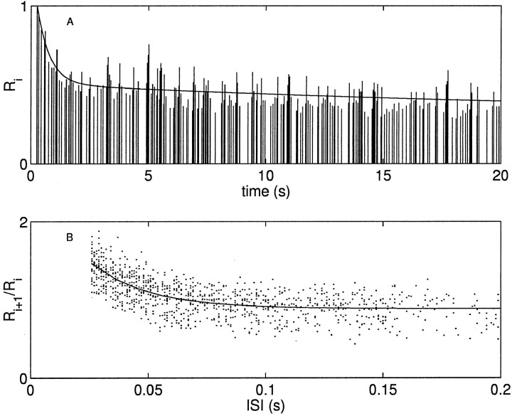
Figure 4A shows the response of a neuron postsynaptic to the interneuron B4/5, which was stimulated to fire action potentials with an exponentially distributed train with a mean rate of 10 Hz. The depression of the resultant IPSCs (Fig. 4A, sticks) can be approximated as the sum of two exponentials (solid line): one with a rate constant of 0.03 s⁻¹, another with a rate constant of 1.81 s⁻¹. In addition there is a facilitation to short interspike intervals (ISIs) that can be well described by a single exponential with a rate constant of 43.5 s⁻¹. In Figure 4B the ratio of adjacent IPSCs (dots) is plotted as a function of ISI. These three influences on short-term plasticity, one time scale for facilitation and two time scales of depression, were seen in all of the neurons investigated that were postsynaptic to B4/5.

Fig. 4.

Postsynaptic response shows two rate constants of depression and one of facilitation. A, The IPSCs (sticks) recorded in a postsynaptic neuron in response to stimulating the presynaptic interneuron B4/5 with a 10 Hz exponentially distributed train of impulses. There are two time scales of depression, one rapidly and the other slowly depressing. Solid line is the best fit to a double exponential function with rate constants 0.03 and 1.81 s⁻¹. The data are normalized by the amplitude of the first IPSC. B, The ratio of the amplitude of an IPSC to that preceding it (dots) plotted as a function of interspike interval. Data are from the entire 120 sec stimulus train of which the first 20 sec are plotted above. Solid line is the best fit to a single exponential function with a rate constant of 43.5 s⁻¹.

Linear model

The simplest model that incorporates two times scales of depression and one of facilitation is linear. In the linear model, the predicted amplitudes are given by the convolution of the impulse train with a linear response function that is the sum of one positive (facilitatory) and two negative (depressing) exponentials with different rate constants:

$$R(t_{\text{i}})=\sum _{\text{j}\le \text{i}} a_1{e}^{-{\alpha }_1({\text{t}}_{\text{i}}-{\text{t}}_{\text{j}})}-a_2{e}^{-{\alpha }_2({\text{t}}_{\text{i}}-{\text{t}}_{\text{j}})}-a_3{e}^{-{\alpha }_3({\text{t}}_{\text{i}}-{\text{t}}_{\text{j}})},$$ Equation 13

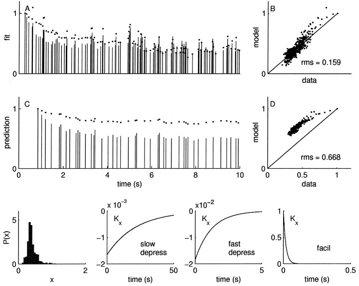
where all of the parameters are positive. This is a special case of Equation 5 where F(x) = x and 𝒜(t_i) = 1. The number of parameters can be reduced to 5 by imposing the normalization R(t₁) = 1. These three exponential functions, and the distribution of the underlying component, are shown in Figure 5, bottom panels.

Fig. 5.

Linear model. IPSC amplitudes are proportional to the convolution of the spike train with a linear response function K_x, which is the sum of three exponential processes: rapid depression, slow depression, and facilitation. The fit is a reasonable first-order approximation with an rms error of 0.15. This is approximately twice as high as the intrinsic variability. A, The vertical sticks are the IPSC magnitudes in the first 10 sec of presynaptic stimulation with 10 Hz train of exponentially distributed impulses; the dots are the best fit of the linear model. B, Data versus model for the entire 60 sec modeled segment. C, D, When the model fit to the data in A and B is used to predict the responses to a novel random stimulus from a different statistical distribution with a different mean frequency (5 Hz train of uniformly distributed intervals), the error is dramatically worse. Bottom panels, The density of the underlying component x and the exponential functions that contribute to kernel K_x: slow depression, rapid depression, and facilitation. The data are normalized by the amplitude of the first IPSC.

Figures 5A shows the first 10 sec of the IPSC response (sticks) to a random stimulus train, and the model fit given by the equation above is plotted with dots. The model versus the data are plotted in Figure 5B, where the identity line indicates a perfect fit. This linear model fits the data with an rms error of 0.15. This is approximately twice the intrinsic neuronal variability, rms error of 0.07 ± 0.02, n = 10 for this neuron, which we measured by computing the variation in the responses of the neuron to identical stimuli (see Materials and Methods; we report mean ± SEM unless indicated otherwise).

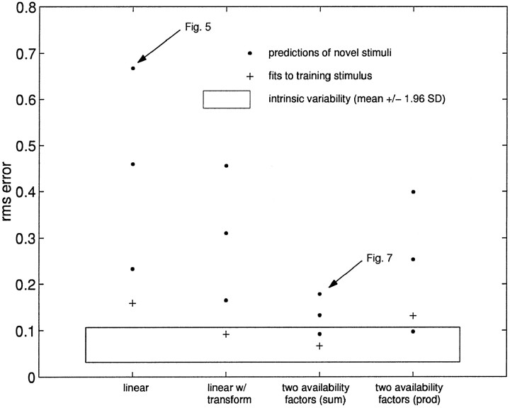
To further test the adequacy of this model, we presented novel stimulus trains having a different mean and interval distribution. The response of the neuron to the novel train is made using the parameters estimated from the training stimulus. An example is shown in Figure 5, C and E. The error of the prediction was 0.67, more than nine times the intrinsic variability. Although the linear model provides an adequate fit to the data in Figure 5, it breaks down entirely on the task of predicting novel stimuli. The data for multiple predictions using the linear model is summarized in Figure6, which shows that both the fit and all predictions fall outside the range expected form the intrinsic neuronal variability (indicated by the bounding box).

Fig. 6.

Model fits and prediction of novel stimuli for four classes of models. Because the data clearly show three time scales of short-term changes in synaptic efficacy (Fig. 4), we looked at several ways in which these time scales can enter into the model presented in Equation 6. Each of the models presented was trained on the same stimulus, a 10 Hz exponential train (+). This model was then used to predict the responses to novel stimuli (●), which were spike trains with different means and interval distributions. Thebounding box shows the range of the intrinsic variability (mean ± 1.96 SD) of the neuron in response to identical stimuli. Although several models provide good fits to the data, the two additive availability factors model is significantly better at predicting responses to novel stimuli. An example of the data for the worst case (linear model) and best case (two additive factors model) is shown in Figures 5 and 7. The number of parameters for the four models shown are 5 (linear), 7 (linear w/transform), and 6 (two factors additive or multiplicative).

Nonlinear transform model

To accurately describe the excitatory junction potential response to repeated stimulation in neuromuscular synapses of the crab, the introduction of a nonlinear transformation (polynomial) of the underlying linear process is a critical step (Sen et al., 1996). Therefore, we investigated a nonlinear transformation F(x(t_i)) given by the Boltzmann function. For values of x below the saturation point, the Boltzmann function has an approximately polynomial shape, but saturates for large values of x. This satisfies the intuitive requirement that the response is bounded. Here again, the availability 𝒜(t_i) = 1 is constant.

Figure 6 shows that this model does a much better job than the linear model, with a fit within the bounds expected from the intrinsic variability of the synaptic response. Again, however, the predictions of responses to novel stimuli are poor.

Availability models

The nonlinear transform model is not designed to handle synapses with availability factors (Sen et al., 1996). We investigated all three of the possible one available factor models that incorporate two time scales of depression. The time scales of depression can be modeled as an accumulation of inhibition in the underlying component x by adding an additional exponential term to the kernel K_x. Alternatively, they can enter into the availability recovery function K_A. Although these three models were able to accurately fit the training stimulus, the mean prediction error, comparable for each model, was approximately rms = 0.2 (range rms = 0.08–0.33; data not shown). This value is roughly four times the intrinsic variability for this neuron.

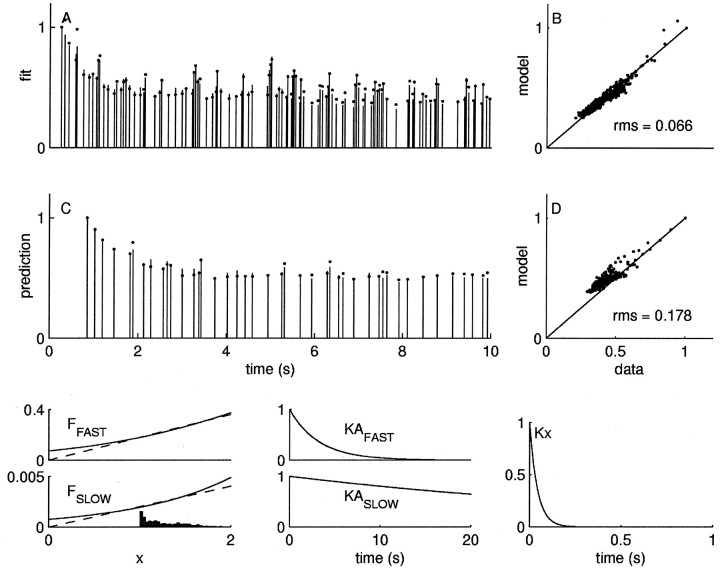
Because the prediction errors of the models with only one availability factor were considerable higher than the intrinsic variability, we investigated a two-factors model with rapidly and slowly recovering availability factors (Fig. 7). This model is given in Equation 6 with n = 2:

$$R(t_{\text{i}})=s_1{F}_1(x(t_{\text{i}})){\mathcal{A}}_1(t_{\text{i}})+s_2{F}_2(x(t_{\text{i}})){\mathcal{A}}_2(t_{\text{i}}).$$ Equation 14

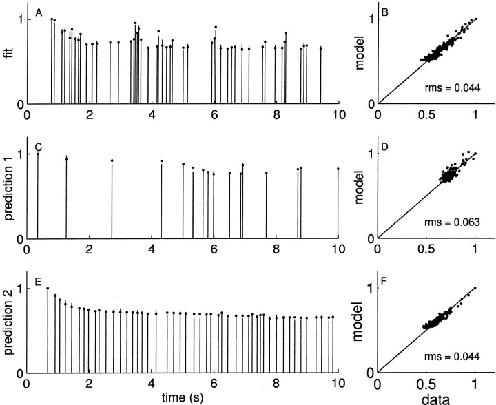
In Figure 7A, the first 10 sec of IPSCs resulting from the training stimulus (same as above) are shown as sticks, and the best fit of the model is shown as dots; the full record of data versus model is shown in Figure 7B. Not only does the model fit the responses to the training stimulus train to within the intrinsic neuronal variability, it also does markedly better at predicting the responses to novel stimuli, as shown in Figure 7, C and D. The data from the fit and multiple predictions are shown in Figure 6.

Fig. 7.

Two-factors model. Plot conventions are described in Figure 5. The model here from Equation 6 provides a twofold better fit (A, B) to the same data in Figure 5 and a fourfold better prediction (C, D) of novel data. Bottom panels, Left, The fraction of the rapid and slow factors activated as a function of the underlying component. Theinset is the density of the underlying component x, with an arbitrary vertical scale. We used the scalar approximation (dashed lines) to the Boltzmann functions (solid lines) to reduce the number of parameters to six so that comparisons between models would be fair. The approximation is quite good over the density of x. Middle, The functions K_A governing the recovery of the rapid and slow factors; right, the function K_x governing the underlying component. The data are normalized by the amplitude of the first IPSC.

We also considered a model in which the two factors combine multiplicatively. Varela et al. (1997) also found two time constants of depression and one of facilitation in excitatory synapses in the neocortex. A multiplicative relationship between the factors described their data. In the neuromuscular junction of frog, there is a multiplicative relationship between augmentation and facilitation (Magleby and Zengel, 1982). Figure 6 shows that the predictions and fit of the two-factors multiplicative model, although better than the linear or linear with transform models, does not fit the data or predict novel stimuli as well as the two-factors additive model. For the rest of the investigations below, we will consider only the two-additive factors model, which we refer to simply as the “two-factors model.”

It should be noted that the number of parameters in the two-factors model (6) is similar to the number of parameters in the other models (5, 6, or 7). It may seem surprising that the two-factors model has the same number of parameters as the one-factor model, rather than twice as many. To describe two time components of depression and one component of facilitation requires several rate constant and amplitude parameters. The difference between the one- and two-factors models is simply where these parameters enter the model. Thus the substantial improvement in the description of the data cannot be attributed to the addition of free parameters.

Rest-time effects

For all experiments, the two-additive factors model consistently predicted the neuronal responses to novel stimuli better than the linear, nonlinear transform, one-factor, or multiplicative models. On closer inspection of the prediction errors of the two-factors model (Figure 6, third column), however, we noted that there was still considerable variability in the goodness of fit. Investigating the possibility that this difference could be attributed to changes in the neuronal state on the time scale of minutes between experiments, we collected a large number of stimulus responses in which we varied the rest-time between stimuli from just under 2 min to >1 hr. Each of the stimuli were long trains lasting several minutes.

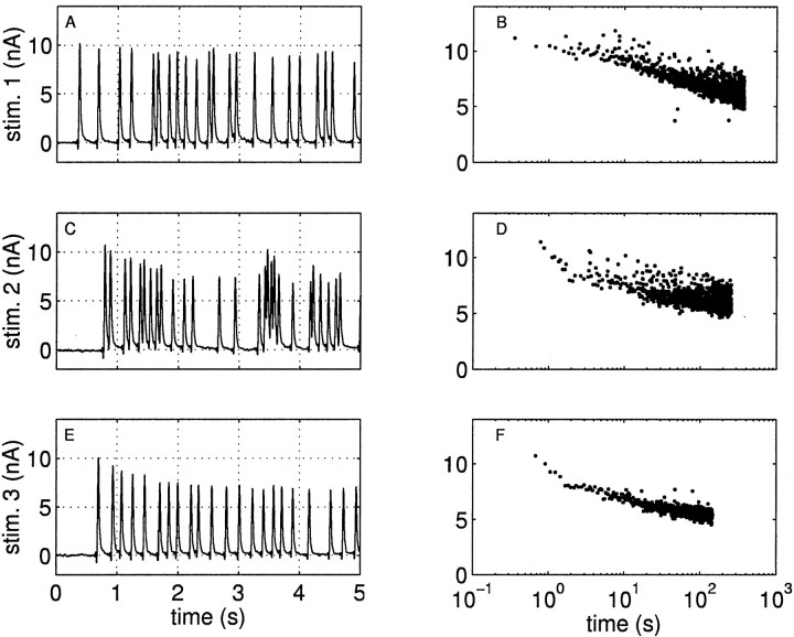
Figure 8A–C shows the response of a neuron to three consecutive stimulus trains drawn from interval distributions having the same mean frequency (5 Hz). In Figure8A, the neuron has rested for >30 min; in Figure 8, B and C, the rest-time was only 2 min. In all cases, there is a slow prolonged decrease in the response throughout the duration of the stimulus train. For the short rest-times, however, an initial rapidly decrementing response of the neuron appears that was not apparent for the rested neuron. Thus the rest-time between stimuli appears to be an important determinant of the extent of synaptic depression in early responses.

Fig. 8.

Responses of a single neuron to three consecutive stimulations of the interneuron B4/5. The left panels show the current traces of the first 5 sec of a much longer stimulation. Theright panels show the amplitudes of IPSCs over the entire stimulus on semilogarithmic axes. All of the stimuli have a mean ISI of 200 msec: A and B show the response to a uniform distribution of intervals with an ISI SD ς = 0.11 sec; C and D show the response to an exponential distribution of intervals with ς = 0.19 sec; E and F show the response to a Gaussian distribution of intervals with ς = 0.078 sec. The smaller variance seen in F compared with B and D presumably arises from the smaller variance in the interval distribution. Note the development on a rapidly depressing component in the first few seconds of the stimulus in the middle and bottom panels, which is not present in the top panel. The top panel is a rested synapse, with >30 min elapsed since the previous stimulus (data not shown), whereas the middle and bottom panelsare comparatively non-rested, with a ≈2 min elapsed since the preceding stimulus. Evidence presented below indicates that the development of a rapidly depressing component is stimulus induced and not dependent on the statistical distribution of the inputs. The apparent increases in the variability of the IPSC amplitudes with time is an illusion created by the use of a logarithmic x -axis. The outliers below the bulk of the responses toward the end of stimuli in B are an artifact. Because these artifacts occurred rarely (≈1/1000 IPSCs), we did not try to remove them from the analysis pool.

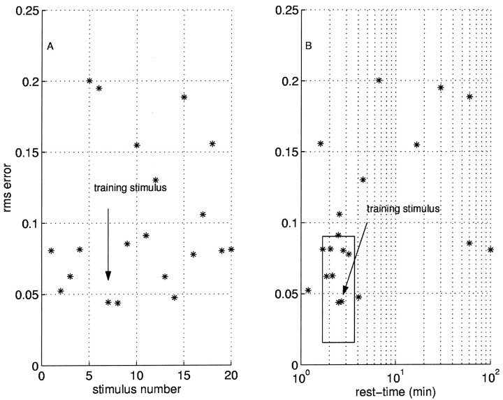
Figure 9 summarizes the prediction error over 20 novel stimuli. The point marked training stimulusindicates the data shown in the top panels of Figure 10. The error in the prediction of the responses to 20 stimuli is plotted as a function of stimulus order (Fig. 9A) and rest-time (Fig.9B). The prediction error is not dependent on stimulus order; the errors appear random as a function of order. However, there is a strong effect of rest-time. For experiments with similar rest-times, indicated by the bounding box in Figure9B, the error in the prediction falls within the expected range given by the intrinsic variability for all points save two.

Fig. 9.

Error in prediction varies with rest-time, not stimulus order. We performed 20 separate stimulations of the same neuron with inputs drawn from different statistical distributions (2 or 5 Hz with exponential, Gaussian, or uniform distribution of intervals). We took 1 of these 20 and trained a two-factors model (training stimulus). A, rms error of the predictions plotted as a function of sequential stimulus number; the error does not vary systematically with order. B, rms error as a function of time since last stimulus (rest-time). The largest prediction errors occur for rest-times far from that of the training stimulus. Thebounding box shows a region where we expect the predictions to be good: the range on the abscissa is given by the rest-time of the training stimulus ± 1 min; the range on theordinate is given be the mean ± 1.96 SDs of the intrinsic variability.

Fig. 10.

Two-factors model predicts responses to novel stimuli. Plot conventions are described in Figure 5. The novel stimuli have a different mean frequency or interval distribution than that used to build the model. The novel stimulus sets were chosen so that their rest-time was similar to that of the training stimulus. A, B, The parameters were determined from the training stimulus. C, D, Model predicts responses to a novel 2 Hz exponentially distributed train. E, F, Model predicts responses to a novel 5 Hz Gaussian distributed train. The data are normalized by the amplitude of the first IPSC.

The training stimulus, with a rest time of ≈2 min, is shown in Figure10A, where the IPSCs are plotted as sticks and the model fits are plotted asdots. Examples of the responses and predictions for two novel stimuli with similar rest-times are shown in Figure 10, C and E. The rms prediction error drops to the order of the intrinsic variability. For each of these three examples, the model predictions versus the measured data for the full segment is plotted to the right.

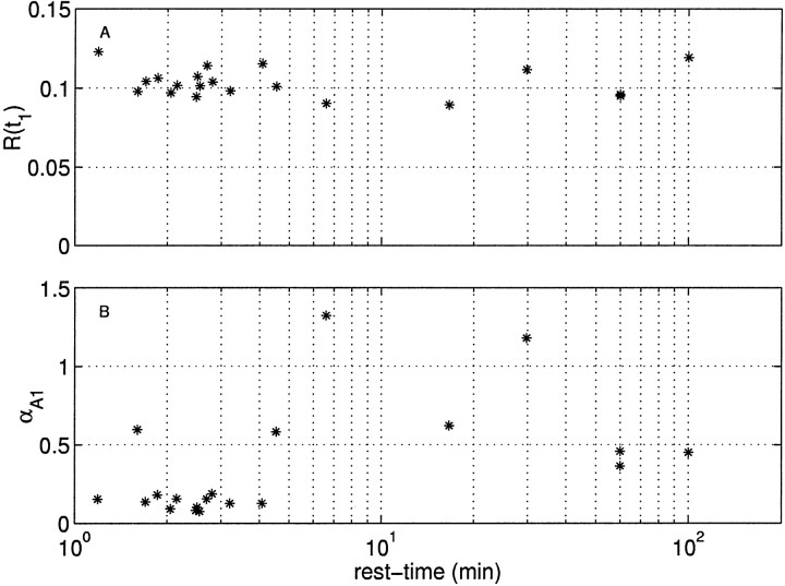
We next determined whether the changes in the response of the neuron attributable to rest-time could be isolated to one of the model components. The observation that the amplitude of the first spike is approximately constant, seen in the raw data in Figure 8, is supported in Figure 11A, where the first spike amplitude over 20 stimulus sets is plotted as a function of rest-time. The proportion of variance in the first IPSC amplitude explained by rest-time is R² = 2%, clearly indicating that the first IPSC does not vary with rest-time.

Fig. 11.

First IPSC amplitude and recovery time constant of rapidly recovering availability factor as a function of rest-time. A, Amplitude of first event. B, Recovery rate constant.

This puts a severe constraint on which parameters can change with rest-time. Namely, only parameters governing recovery can change without systematically altering first IPSC amplitude. Thus, if we assume that only one parameter is changing with rest-time (see Discussion), this leaves the parameters governing K_x, K_A1, and K_A2 as candidates. These kernels govern the decay of the underlying component, the recovery rate of the rapid factor, and the recovery rate of the slow factor. The rate constants for these three kernels are α_x, α_A1, and α_A2.

The procedure to identify the parameter that varied with rest-time is as follows. By sharing five of the six model parameters between stimuli, and allowing one (α_x, α_A1, or α_A2) to vary freely, we simultaneously fit the model to all stimuli over the range of rest-times. We found that only α_A1 was sufficient to account for the changing response with rest-time, with an overall rms error of 0.05 ± 0.007, n = 20 equivalent to the intrinsic variability. The rms error obtained when only α_A1 was allowed to vary was significantly lower than that obtained with either α_A2 or α_x (Student's t test; p < 0.01; n = 20). The latter two were statistically indistinguishable.

Figure 11B shows the recovery time constant as a function of rest-time. For short times, the time constant is small (with one exception) and grows with longer rest-times. There is, however, considerable variability with long rest-times. The simplest explanation consistent with our observations is that presynaptic stimulation of B4/5 slows the rate of recovery of the rapid factor.

How are two neurons different?

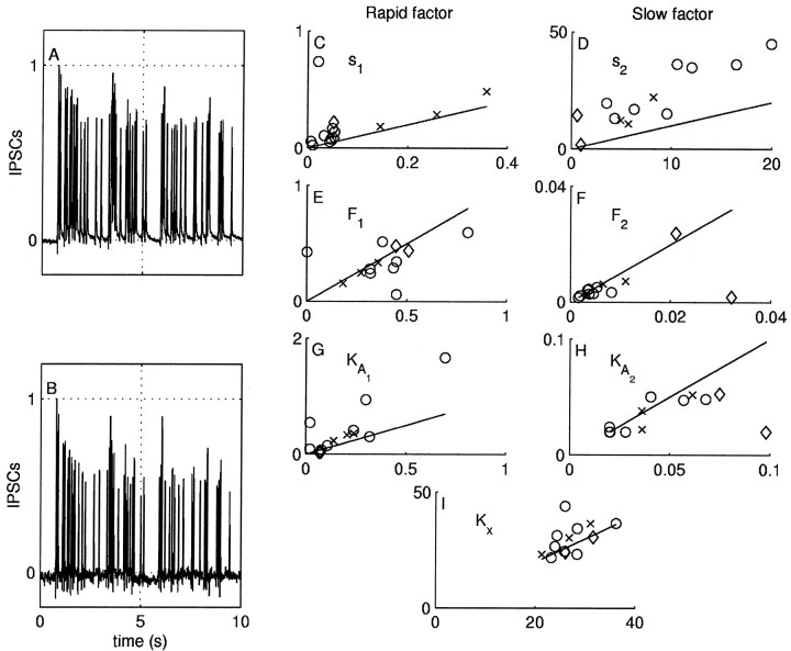
Figure 12, A and B, shows IPSCs recorded simultaneously in two neurons postsynaptic to the B4/5, which was stimulated to fire action potentials with a 5 Hz Poisson stimulus. Despite the fact that both neurons are postsynaptic to the same interneuron, their responses are quantitatively different. In particular, for one of the neurons, the depression of the IPSC amplitudes in the early response is clearly larger.

Fig. 12.

Responses of two postsynaptic neurons recorded simultaneously in response to stimulation of B4/5. A, B, IPSCs from a 10 sec segment of a random stimulus train. The amplitude of the currents in both neurons is normalized by the first event to facilitate comparison. Both neurons show similar features, notably an initial rapid depression and a sustained slow depression, as well as short-term facilitation after short interspike intervals. The rapid onset of depression in the lower neuron, however, is more pronounced. C–I, Plots of the parameter values from one neuron versus the other. The neuron with the smaller average IPSC in each pair is assigned plotted along the ordinate, and other neuron in the pair is plotted along the abscissa. A full two-additive factors model was fit to each neuron in the pair, and the values for each of the seven parameters are plotted. Multiple stimuli for each pair are plotted with the symbols ×, ◊, and ○, indicating the neuron pair. Values that fall along the identity line indicate that both neurons in the pair have identical values for that parameter.

A useful way to estimate the difference between the IPSC amplitudes of the two neurons is to again use the rms error. Identifying one of the trains with the “prediction,” the rms error of the second relative to the first is 0.25. This error is approximately five times the intrinsic neuronal variability (0.05 and 0.06 for the neurons in Fig.12). The average rms difference between the two neurons in all pairs investigated, normalizing the IPSCs in each train by the first, is 0.20 ± 0.03, n = 13. Thus the differences in the response between the two neurons cannot be explained simply in terms of random variations in neuronal response.

To quantify the differences between the neurons in terms of the model, we fit the parameters of the model to each neuron pair for all pairs. Unlike the case above, in which we investigated how a single neuron changes with rest-time, in the two-neuron case the amplitude of the first IPSC is not the same between neurons. So we did not constrain the investigation to rate constants. Instead, we modeled each postsynaptic neuron independently.

For each pair of simultaneously recorded responses, we assigned the response with the smaller average IPSC to be neuron 1 and the other to be neuron 2. The values for each of the parameters are plotted in Figure 12C–I, in which the parameter value for neuron 1 is plotted along the abscissa and the value for neuron 2 is plotted along the ordinate. The line of identity indicates the values where the two neurons have the same value for the parameter plotted. The left column (C, E, G) shows the parameters for the rapid factor, and the right column (D, F, H) shows the parameters for the slow factor. The data are taken from 13 stimuli in three neuron pairs (plotted with the symbols ×, ◊, and ○). A given neuron may change from stimulus to stimulus, as noted in the discussion of rest-time effects above. For both scalar factors s₁ and s₂, the values for neuron 2 are consistently larger than for neuron 1, falling above the line of identity (Fig. 12C,D); this is particularly apparent for s₂. Although there is considerable scatter about the line of identity for the other parameters, there are no consistent differences between neuron pairs.

We then tested to see whether variations s₁ and s₂ alone could account for the different responses by constraining the model for each pair to share all parameters except s₁ and s₂. If the model can fit the data to within the bounds expected by the intrinsic variability with this constraint, then this suggests that these two parameters are sufficient to explain interneuronal variation. With these constraints, the average fit rms error was 0.07 ± 0.01, n = 13, which is within the intrinsic variability bounds. These observations suggest that the main difference between the two neurons can be accounted for by the amount of current carried by the rapid and slow factors.

DISCUSSION

One of the fundamental issues in the study of neural computation is the information flow across the synapse. The model presented here accurately describes the output of a central synapse to a wide range of synaptic inputs, varying in mean and interval distributions. Although the model does not identify the locus of these factors, this distinction may not be important for the study of computation and information transfer, because it is the total synapse that is the operative unit. The model does identify, however, how many availability factors are required to describe the synapse, their relative sizes, and recovery kinetics. It also provides a means to assess how these quantities change with experimental perturbations. Many different possible mechanisms can give rise to similar qualitative behavior. Thus, a mechanism-independent means of quantifying synaptic properties is useful.

Our results imply the existence of two availability factors at the B4/5 synapse of Aplysia. The smaller factor is characterized by a high probability of activation and a recovery time of the order of seconds. This factor governs the rapid depression seen in the early IPSC response. Changes in the recovery rate of this factor can explain the effects of rest-time on neuronal response. The larger factor is characterized by a lower probability of activation and recovers with a time course on the order of tens of seconds. This factor generates the long slow decay of the response seen throughout the several hundred seconds of stimulation. These observations are qualitatively similar to those of Varela et al. (1997) in visual cortex, who also observed two time scales of depression and one of facilitation.

We have shown that a model of the Aplysia central synapse that incorporates these two availability factors together with a single facilitation component describes the response of the neurons to both training and novel spike trains. This model does not distinguish between availability factors located presynaptically from those located postsynaptically. The fact that both factors share the same underlying component and are otherwise independent, however, suggests that they are on the same side of the synapse. In other systems, there is abundant evidence supporting the existence of multiple pools of vesicles (Mennerick and Matthews, 1996; Silver et al., 1998; Gomis et al., 1999; Burrone and Lagnado, 2000; Stevens and Williams, 2000); for reviews, see Zucker (1996) and Neher (1998). Although we cannot exclude the possibility that the dynamics observed in our preparation arise from presynaptic depression or vesicle depletion, we have chosen to discuss our results in the context of the known properties of Aplysia acetylcholine receptors (AChRs) in B4/5 follower neurons.

In Aplysia, early work indicated the presence of at least two pharmacologically distinct AChRs, with different desensitization sensitivities (Tauc and Gerschenfeld, 1961; Tauc and Bruner, 1963; Kehoe, 1969). In the buccal ganglion follower cells of B4/5, two different AChRs on the same neuron have different rates of desensitization to repeated stimulation of B4/5; this can be mimicked with ionophoretic acetylcholine (ACh) application (Gardner and Kandel, 1977). Selective antagonization of one of two classes of pharmacologically distinct AChRs, each of which mediate an inhibitory Cl⁻conductance, reveals that one rapidly desensitizes to tonic ACh application, whereas the other slowly desensitizes (Kehoe and McIntosh, 1998). In the cholinergic buccal neurons thatKehoe and McIntosh (1998) investigated, it appeared that the two receptor populations were present in different proportions. The multicomponent response is by no means limited to Aplysia, but rather is a common feature of postsynaptic responses (Feigenspan and Bormann, 1994; Elson and Selverston, 1995; McGehee and Role, 1995).

Thus the evidence on desensitization of AChRs in Aplysia is consistent with our observations. There are two populations of inhibitory receptors with different desensitization sensitivities, and there is neuronal variation in the proportion of these two populations. This is consistent with the model findings that the sizes of the two availability factors varied between neurons. We also found that stimulation of B4/5 led to a more rapid depression of the early responses in subsequent trains. In the model, this was identified with a slowing of the rate of recovery of the rapidly recovering factor. Under the desensitization hypothesis, this predicts that repeated application of ACh slows the recovery from desensitization for the rapidly desensitizing inhibitory AChRs.

Although it might be anticipated that in a prolonged train the shape of the IPSC waveform would change during receptor desensitization (which we did not observe), this does not always occur. For example, in central GABAergic synapses, there is a slow GABA_A receptor desensitization that affects only the IPSC amplitude (Overstreet et al., 2000). Additionally, the rapid effects of acetylcholinesterase at buccal cholinergic synapses may serve to block such actions of acetylcholine (Simonneau and Tauc, 1987;Fossier et al., 1990).

Our conclusion that stimulation modulates the recovery rate of the rapid factor is based on the assumption that only one parameter is changing with rest-time. Other explanations are possible. If more than one parameter is allowed to vary simultaneously, then the stimulus-induced changes can be explained, for example, by allowing the sizes of both factors to vary with rest-time. As long as the relative sizes are constrained so that the amplitude of the first IPSC is approximately constant, the stimulus-induced modulation of depression can be modeled as an increase in the proportion of the rapid factor (data not shown). This raises the possibility that differential sensitivity to the stimulus-induced changes contributes to the observed synaptic heterogeneity. Such stimulus-dependent control of receptor expression is observed in other systems, where the cycling of receptors shows differential sensitivity to stimulus modulation depending on receptor type (Turrigiano et al., 1998; Akaaboune et al., 1999; Ehlers, 2000).

It is experimentally challenging to measure the properties of synapses in which the stimuli themselves alter the synaptic response to subsequent stimuli. We observed that long trains of stimuli had effects on synaptic depression that persisted over a time scale of minutes. These effects cannot be readily quantified using paired-pulse stimulation, for example, because the effect decays during the time it takes to measure it. Protocols that measure synaptic properties at longer time scales magnify the difficulties. Although it is possible in some specialized systems to eliminate this confound with clever experimental protocols (Rosenmund and Stevens, 1996), it remains a general problem. Our approach provides a solution by allowing synaptic processes over a range of time scales to be quantified with a single, short stimulus train.

The generalization of the synaptic decoding optimization methodology to multiple availability factors provides a powerful tool to investigators in various systems. For mechanistic investigations, the available factors model and optimization methodology can be used with narrowly focused experimental preparations, where the presynaptic or postsynaptic side can be isolated experimentally. It may be used equally well where synaptic activity is assayed with postsynaptic currents, presynaptic capacitance changes, fluorescence increases, or any other measurement where the data can be represented as a series of times and amplitudes.

The use of the additive multiple factors also solves a recurring problem with one-factor models: they often overestimate the amount of depression in prolonged trains. One approach to solving this problem is to incorporate a stimulus/calcium-dependent increase in the recovery rate of the availability factor (Byrne, 1982;Dittman and Regehr, 1998). Another is to assume that the probability of release is very small (Brezina et al., 2000b). This latter approach, however, cannot account for synapses that show an initial rapid depression and a sustained response. We encountered a similar problem with the two multiplicative factors model (Varela et al., 1997), which assumes that the response is given by the product of facilitation and two depression factors. Although this model was able to fit the bulk of the IPSCs (those occurring after the initial rapid depression), it tended to underestimate the first several spikes, or if we applied the first IPSC amplitude constraint given in Equation 9, the subsequent several spikes were consistently overestimated. In short, we found it difficult with this model to obtain accurate fits of both the initial rapid depression and the slower sustained depression. The two-factors model with additive rapid and slow factors provides an alternate solution that satisfies both time scales of depression.

Responses of the central and peripheral synapses depend on their past history. A consequence is that the same spike train presented to the same neuron at different times will likely generate different responses. To complicate matters, the response is highly dependent on the statistical properties of the spike train. To highlight an extreme case, a low-frequency synaptic input to a neuron in the abdominal ganglion of Aplysia generates an excitatory response, whereas a high-frequency input at the same synapse generates an inhibitory response, because of presence of two populations of receptors with different desensitization rates (Wachtel and Kandel, 1971). Observations such as these limit the utility of attempts to unravel the nature of the neural code from action potential times alone, because the effects of these action potentials depend heavily on dynamic synaptic properties.

Gradients for parameter optimization

One-factor model

Here we provide the expressions for the partial derivatives of the model R in Equation 5 with respect to the parameters controlling s, F, and 𝒜. These partials are used in computing the gradient of the model error given in Equation 12. Because the availability 𝒜 is defined recursively in Equation 4, the gradient of the response must be defined recursively as well. We begin with the assumption that 𝒜(t₁) = 1; that is, there is full availability of the factor at the time of the first spike.

The partial derivative of Equation 5 with respect to any parameter α is, by the product rule:

$$\frac{\partial R}{\partial \alpha }(t_{\text{i}})=\frac{\partial s}{\partial \alpha }(t_{\text{i}})F(x(t_{\text{i}}))\mathcal{A}(t_{\text{i}})+s \frac{\partial F}{\partial \alpha }(x(t_{\text{i}}))\mathcal{A}(t_{\text{i}})+\text{sF}(x(t_{\text{i}}))\frac{\partial \mathcal{A}}{\partial \alpha }(t_{\text{i}}).$$ Equation 15

The partial derivative of s:

$$\frac{\partial s}{\partial \alpha }(t_{\text{i}})=1\hspace{1em}\alpha \equiv s$$ Equation 16

$$=0\hspace{1em}\text{otherwise}.$$

The partial derivatives of 𝒜:

$$\frac{\partial \mathcal{A}}{\partial \alpha } (t_{\text{i}+1})=-\frac{\partial K_A}{\partial \alpha }(\mathrm{\Delta }t)[1-\mathcal{A}(t_{\text{i}})(1-F(x(t_{\text{i}})))]\alpha \text{controls} K_A$$

$$+K_A(\mathrm{\Delta }t)\frac{\partial \mathcal{A}}{\partial \alpha }(t_{\text{i}})(1-F(x(t_{\text{i}})))$$ Equation 17

$$=K_A(\mathrm{\Delta }t)\begin{array}{c}\left[\frac{\partial \mathcal{A}}{\partial \alpha }(t_{\text{i}})(1-F(x(t_{\text{i}})))\right.\\ \hfill -\mathcal{A}(t_{\text{i}})\left.\frac{\partial F}{\partial \alpha }(x(t_{\text{i}}))\right]\hfill \end{array}\hspace{1em}\alpha \text{controls} F$$

$$=0\hspace{1em}\text{otherwise},$$

where Δt = t_i+1 − t_i.

The partial derivatives of F:

$$\frac{\partial F}{\partial \alpha }(x(t_{\text{i}}))\equiv \frac{\partial F}{\partial \alpha }(x(t_{\text{i}}))\alpha \text{controls} F$$ Equation 18

$$=\frac{\text{d}F}{\text{d}x}(x(t_{\text{i}}))\frac{\partial x}{\partial \alpha }(t_{\text{i}})\alpha \text{controls} x,$$ Equation 19

where, from Equation 1:

$$\frac{\partial x}{\partial \alpha }(t_{\text{i}})=\sum _{{\text{t}}_{\text{j}}\le {\text{t}}_{\text{i}}} \frac{\partial K_{\text{x}}}{\partial \alpha }(t_{\text{i}}-t_{\text{j}}).$$ Equation 20

Because the gradients in Equation 17 are defined recursively, we must define the values of 𝒜(t₁) and F( x(t₁)). Because the initial availability is constant, ∂𝒜(t₁)/∂α = 0 for all parameters, and ∂F(x(t₁))/∂α can be obtained from the expressions in Equation 18.

Multiple-factors model: additive

The partial derivatives of the additive multiple factor model given in Equation 6 follow directly because the N factors sum linearly

$$\frac{\partial R}{\partial \alpha }(t_{\text{i}})=\sum _{\text{j}=1}^N \frac{\partial R_{\text{j}}}{\partial \alpha }(t_{\text{i}}),$$ Equation 21

where the expression for ∂R_j(t_i)/∂α is given in Equation 15.

In the case of the constrained model given in Equation7, however, the following expression for ∂s_N(t_i)/∂α must be used in place of the one given in Equation 16:

$$\frac{\partial s_N}{\partial \alpha }(t_{\text{i}})=-\sum _{\text{j}=1}^{N-1} \frac{\partial R_{\text{j}}}{\partial \alpha }(t_1)/(F_N(x(t_1)){\mathcal{A}}_N(t_1))$$ Equation 22

$$-s_N\left(\frac{\partial F_N}{\partial \alpha }(x(t_1))/F_N(x(t_1))+\frac{\partial {\mathcal{A}}_N}{\partial \alpha }(t_1)/{\mathcal{A}}_N(t_1)\right).$$

This expression follows directly from the requirement that ∂R(t₁)/∂α = 0 for all parameters because R(t₁) is constant in the constrained model. Note that ∂F_N(x(t₁))/∂α = 0 for all parameters except those governing F_N and the underlying component x. ∂𝒜_N(t₁)/∂α = 0 for all parameters, because we assume that the initial availability is a constant.

Multiple factors model: multiplicative

The partial derivatives of the multiplicative multiple factor model given in Equation 8 are given by:

$$\frac{\partial R}{\partial \alpha }(t_{\text{i}})=\sum _{\text{j}=1}^N \frac{\partial R_{\text{j}}}{\partial \alpha }({\text{t}}_{\text{i}})\prod _{\text{k}=1,\text{k}\ne \text{j}}^N R_{\text{k}}(t_{\text{i}})$$ Equation 23

$$=R \sum _{\text{j}=\text{i}}^N \frac{\partial R_{\text{j}}}{\partial \alpha }({\text{t}}_{\text{i}})/R_{\text{j}}(t_{\text{i}}),$$ Equation 24

where the expression for ∂R_j(t_i)/∂α is given in Equation 15.

The partial of s_N below, when using the constraint given in Equation 9, must be used in place of the one given in Equation 16:

$$\frac{\partial s_N}{\partial \alpha }(t_{\text{i}})=s_N\left(\frac{\partial {\mathcal{A}}_N}{\partial \alpha }(t_1)/{\mathcal{A}}_N(t_1)+\frac{\partial P_N}{\partial \alpha }(t_1)/P_N(t_1)-\sum _{\text{j}=1}^{N-1} \frac{\partial R_{\text{j}}}{\partial \alpha }(t_1)/R_{\text{j}}(t_1)\right).$$ Equation 25

REFERENCES

- 1.Abarbanel HD, Huerta R, Rabinovich MI, Rulkov NF, Rowat PF, Selverston AI. Synchronized action of synaptically coupled chaotic model neurons. Neural Comput. 1996;8:1567–1602. doi: 10.1162/neco.1996.8.8.1567. [DOI] [PubMed] [Google Scholar]
- 2.Abbott LF, Varela JA, Sen K, Nelson SB. Synaptic depression and cortical gain control. Science. 1997;275:220–224. doi: 10.1126/science.275.5297.221. [DOI] [PubMed] [Google Scholar]
- 3.Akaaboune M, Culican S, Turney S, Lichtman J. Rapid and reversible effects of activity on acetylcholine receptor density at the neuromuscular junction in vivo. Science. 1999;286:503–506. doi: 10.1126/science.286.5439.503. [DOI] [PubMed] [Google Scholar]
- 4.Berger TW, Eriksson JL, Ciarolla DA, Sclabassi RJ. Nonlinear systems analysis of the hippocampal perforant path-dentate projection. II. Effects of random impulse train stimulation. J Neurophysiol. 1988;60:1076–1094. doi: 10.1152/jn.1988.60.3.1077. [DOI] [PubMed] [Google Scholar]
- 5.Bressloff PC. Mean-field theory of globally coupled integrate-and-fire neural oscillators with dynamic synapses. Phys Rev E. 1999;60:2160–2170. doi: 10.1103/physreve.60.2160. [DOI] [PubMed] [Google Scholar]
- 6.Brezina V, Orekhova IV, Weiss KR. The neuromuscular transform: the dynamic, nonlinear link between motor neuron firing patterns and muscle contraction in rhythmic behaviors. J Neurophysiol. 2000a;83:207–231. doi: 10.1152/jn.2000.83.1.207. [DOI] [PubMed] [Google Scholar]
- 7.Brezina V, Church PJ, Weiss KR. Temporal pattern dependence of neuronal peptide transmitter release: models and experiments. J Neurosci. 2000b;20:6760–6772. doi: 10.1523/JNEUROSCI.20-18-06760.2000. [DOI] [PMC free article] [PubMed] [Google Scholar]
- 8.Burrone J, Lagnado L. Synaptic depression and the kinetics of exocytosis in retinal bipolar cells. J Neurosci. 2000;20:568–578. doi: 10.1523/JNEUROSCI.20-02-00568.2000. [DOI] [PMC free article] [PubMed] [Google Scholar]
- 9.Byrne JH. Analysis of synaptic depression contributing to habituation of gill-withdrawal reflex in Aplysia Californica. J Neurophysiol. 1982;48:431–438. doi: 10.1152/jn.1982.48.2.431. [DOI] [PubMed] [Google Scholar]
- 10.Castillo PE, Katz B. Quantal components of the end-plate potential. J Physiol (Lond) 1954;124:560–573. doi: 10.1113/jphysiol.1954.sp005129. [DOI] [PMC free article] [PubMed] [Google Scholar]
- 11.Chance FS, Nelson SB, Abbott LF. Synaptic depression and the temporal response characteristics of V1 cells. J Neurosci. 1998;18:4785–4799. doi: 10.1523/JNEUROSCI.18-12-04785.1998. [DOI] [PMC free article] [PubMed] [Google Scholar]
- 12.Church PJ, Lloyd PE. Activity of multiple identified motor neurons recorded intracellularly during evoked feedinglike motor programs in Aplysia. J Neurophysiol. 1994;72:1794–1809. doi: 10.1152/jn.1994.72.4.1794. [DOI] [PubMed] [Google Scholar]
- 13.Cleland TA, Selverston AI. Dopaminergic modulation of inhibitory glutamate receptors in the lobster stomatogastric ganglion. J Neurophysiol. 1997;78:3450–3452. doi: 10.1152/jn.1997.78.6.3450. [DOI] [PubMed] [Google Scholar]
- 14.Dittman JS, Regehr WG. Calcium dependence and recovery kinetics of presynaptic depression at the climbing fiber to Purkinje cell synapse. J Neurosci. 1998;18:6147–6162. doi: 10.1523/JNEUROSCI.18-16-06147.1998. [DOI] [PMC free article] [PubMed] [Google Scholar]
- 15.Ehlers MD. Reinsertion or degradation of AMPA receptors determined by activity-dependent endocytic sorting. Neuron. 2000;28:511–525. doi: 10.1016/s0896-6273(00)00129-x. [DOI] [PubMed] [Google Scholar]
- 16.Elson RC, Selverston AI. Slow and fast synaptic inhibition evoked by pattern-generating neurons of the gastric mill network in spiny lobsters. J Neurophysiol. 1995;74:1996–2011. doi: 10.1152/jn.1995.74.5.1996. [DOI] [PubMed] [Google Scholar]
- 17.Feigenspan A, Bormann J. Differential pharmacology of GABAA and GABAC receptors on rat retinal bipolar cells. Eur J Pharmacol. 1994;288:97–104. doi: 10.1016/0922-4106(94)90014-0. [DOI] [PubMed] [Google Scholar]
- 18.Fletcher R. Practical methods of optimization. Wiley; New York: 1987. [Google Scholar]
- 19.Fossier P, Baux G, Poulain B, Tauc L. Receptor-mediated presynaptic facilitation of quantal release of acetylcholine induced by pralidoxime in Aplysia. Cell Mol Neurobiol. 1990;10:383–404. doi: 10.1007/BF00711182. [DOI] [PubMed] [Google Scholar]
- 20.Gardner D. Variations in amplitude and time course of inhibitory postsynaptic currents. J Neurosci. 1986;16:1424–1438. doi: 10.1152/jn.1986.56.5.1424. [DOI] [PubMed] [Google Scholar]
- 21.Gardner D. Paired individual and mean postsynaptic currents recorded in four-cell networks of Aplysia. J Neurosci. 1990;10:1226–1240. doi: 10.1152/jn.1990.63.5.1226. [DOI] [PubMed] [Google Scholar]
- 22.Gardner D, Kandel ER. Physiological and kinetic properties of cholinergic receptors activated by multiaction interneurons in buccal ganglia of Aplysia. J Neurosci. 1977;17:333–348. doi: 10.1152/jn.1977.40.2.333. [DOI] [PubMed] [Google Scholar]
- 23.Gillary HL, Kennedy D. Neuromuscular effects of impulse pattern in a crustacean motoneuron. J Neurophysiol. 1969;32:607–612. doi: 10.1152/jn.1969.32.4.607. [DOI] [PubMed] [Google Scholar]
- 24.Gomis A, Burrone J, Lagnado L. Two actions of calcium regulate the supply of releasable vesicles at the ribbon synapse of retinal bipolar cells. J Neurosci. 1999;19:6309–6317. doi: 10.1523/JNEUROSCI.19-15-06309.1999. [DOI] [PMC free article] [PubMed] [Google Scholar]
- 25.Hill AA, Jin P. Regulation of synaptic depression rates in the cricket cercal sensory system. J Neurosci. 1998;18:1277–1285. doi: 10.1152/jn.1998.79.3.1277. [DOI] [PubMed] [Google Scholar]
- 26.Hung G, Stark L, Eykhoff P. On the interpretation of kernels. I. Computer stimulation of responses to impulse pairs. Ann Biomed Eng. 1977;5:130–143. doi: 10.1007/BF02364013. [DOI] [PubMed] [Google Scholar]
- 27.Hunter JD, Milton JG, Thomas PJ, Cowan JD. Resonance effect for neural spike time reliability. J Neurophysiol. 1998;80:1427–1438. doi: 10.1152/jn.1998.80.3.1427. [DOI] [PubMed] [Google Scholar]
- 28.Jorge-Rivera JC, Sen K, Birmingham JT, Abbott LF, Marder E. Temporal dynamics of convergent modulation at a crustacean neuromuscular junction. J Neurophysiol. 1998;80:2559–2570. doi: 10.1152/jn.1998.80.5.2559. [DOI] [PubMed] [Google Scholar]
- 29.Kehoe J. Single presynaptic neurone meditates a two component postsynaptic inhibition. Nature. 1969;221:866–868. doi: 10.1038/221866a0. [DOI] [PubMed] [Google Scholar]
- 30.Kehoe J, McIntosh JM. Two distinct nicotinic receptors, one pharmacologically similar to the vertebrate α7-containing receptor, mediate Cl currents in Aplysia neurons. J Neurosci. 1998;18:8198–8213. doi: 10.1523/JNEUROSCI.18-20-08198.1998. [DOI] [PMC free article] [PubMed] [Google Scholar]
- 31.Krausz HI. Identification of nonlinear systems using random impulse train inputs. Biol Cybern. 1975;19:217–230. [Google Scholar]
- 32.Krausz HI, Friesen WO. The analysis of nonlinear synaptic transmission. J Gen Physiol. 1977;70:243–265. doi: 10.1085/jgp.70.2.243. [DOI] [PMC free article] [PubMed] [Google Scholar]
- 33.Liley A, North K. Depression and recovery of transmission at the squid giant synapse. J Neurophysiol. 1953;16:509–527. [Google Scholar]
- 34.Magleby KL, Zengel JE. A quantitative description of stimulation-induced changes in transmitter release at the frog neuromuscular junction. J Gen Physiol. 1982;80:613–638. doi: 10.1085/jgp.80.4.613. [DOI] [PMC free article] [PubMed] [Google Scholar]
- 35.Markram H, Wang Y, Tsodyks M. Differential signaling via the same axon of neocortical pyramidal neurons. Proc Natl Acad Sci USA. 1998;95:5323–5328. doi: 10.1073/pnas.95.9.5323. [DOI] [PMC free article] [PubMed] [Google Scholar]
- 36.McGehee DS, Role LW. Physiological diversity of nicotinic acetylcholine receptors expressed by vertebrate neurons. Annu Rev Physiol. 1995;57:521–546. doi: 10.1146/annurev.ph.57.030195.002513. [DOI] [PubMed] [Google Scholar]
- 37.Mennerick S, Matthews G. Ultrafast exocytosis elicited by calcium current in synaptic terminals of retinal bipolar neurons. Neuron. 1996;17:1241–1249. doi: 10.1016/s0896-6273(00)80254-8. [DOI] [PubMed] [Google Scholar]
- 38.Neher E. Vesicle pools and Ca2+ microdomains: new tools for understanding their roles in neurotransmitter release. Neuron. 1998;20:389–399. doi: 10.1016/s0896-6273(00)80983-6. [DOI] [PubMed] [Google Scholar]
- 39.Neiman A, Pei X, Russell D, Wojtenek W, Wilkens L, Moss F, Braun HA, Huber MT, Voigt K. Synchronization of the noisy electrosensitive cells in the paddlefish. Phys Rev Lett. 1999;82:660–663. [Google Scholar]
- 40.Neves G, Lagnado L. The kinetics of exocytosis and endocytosis in the synaptic terminal of goldfish retinal bipolar cells. J Physiol (Lond) 1999;515:181–202. doi: 10.1111/j.1469-7793.1999.181ad.x. [DOI] [PMC free article] [PubMed] [Google Scholar]
- 41.O'Donovan MJ, Rinzel J. Synaptic depression: a dynamic regulator of synaptic communication with varied functional roles. Trends Neurosci. 1997;20:431–433. doi: 10.1016/s0166-2236(97)01124-7. [DOI] [PubMed] [Google Scholar]
- 42.Ogura H. Orthogonal functions of the poisson process. IEEE Trans Info Theory. 1972;18:473–481. [Google Scholar]
- 43.Overstreet LS, Jones MV, Westbrook GL. Slow desensitization regulates the availability of synaptic GABAA receptors. J Neurosci. 2000;20:7914–7921. doi: 10.1523/JNEUROSCI.20-21-07914.2000. [DOI] [PMC free article] [PubMed] [Google Scholar]
- 44.Rosenmund C, Stevens CF. Definition of the readily releasable pool of vesicles at hippocampal synapses. Neuron. 1996;16:1197–1207. doi: 10.1016/s0896-6273(00)80146-4. [DOI] [PubMed] [Google Scholar]
- 45.Sclabassi RJ, Eriksson JL, Port RL, Robinson GB, Berger TW. Nonlinear systems analysis of the hippocampal perforant path-dentate projection. I. Theoretical and interpretational considerations. J Neurophysiol. 1988;60:1066–1076. doi: 10.1152/jn.1988.60.3.1066. [DOI] [PubMed] [Google Scholar]
- 46.Sen K, Jorge-Rivera JC, Marder E, Abbott LF. Decoding synapses. J Neurosci. 1996;16:6307–6318. doi: 10.1523/JNEUROSCI.16-19-06307.1996. [DOI] [PMC free article] [PubMed] [Google Scholar]
- 47.Silver RA, Momiyama A, Cull-Candy SG. Locus of frequency-dependent depression identified with multiple-probability fluctuation analysis at rat climbing fibre-Purkinje cell synapses. J Physiol (Lond) 1998;510:881–902. doi: 10.1111/j.1469-7793.1998.881bj.x. [DOI] [PMC free article] [PubMed] [Google Scholar]
- 48.Simonneau M, Tauc L. Properties of miniature postsynaptic currents during depolarization-induced release at a cholinergic neuroneuronal synapse. Cell Mol Neurobiol. 1987;7:175–190. doi: 10.1007/BF00711553. [DOI] [PubMed] [Google Scholar]
- 49.Stevens CF, Wesseling JF. Activity-dependent modulation of the rate at which synaptic vesicles become available to undergo exocytosis. Neuron. 1998;21:415–424. doi: 10.1016/s0896-6273(00)80550-4. [DOI] [PubMed] [Google Scholar]
- 50.Stevens CF, Williams JH. “Kiss and run” exocytosis at hippocampal synapses. Proc Natl Acad Sci USA. 2000;97:12828–12833. doi: 10.1073/pnas.230438697. [DOI] [PMC free article] [PubMed] [Google Scholar]
- 51.Tauc L, Bruner J. “Desensitization” of cholinergic receptors by acetylcholine in molluscan central neurones. Nature. 1963;198:33–34. doi: 10.1038/198033a0. [DOI] [PubMed] [Google Scholar]
- 52.Tauc L, Gerschenfeld HM. Cholinergic transmission mechanisms for both excitation and inhibition in molluscan central synapses. Nature. 1961;192:366–367. doi: 10.1038/192366a0. [DOI] [PubMed] [Google Scholar]
- 53.Tsodyks M, Uziel A, Markram H. Synchrony generation in recurrent networks with frequency-dependent synapses. J Neurosci. 2000;20:RC50. doi: 10.1523/JNEUROSCI.20-01-j0003.2000. [DOI] [PMC free article] [PubMed] [Google Scholar]
- 54.Turrigiano GG, Leslie KR, Desai NS, Rutherford LC, Nelson SB. Activity-dependent scaling of quantal amplitude in neocortical neurons. Nature. 1998;391:892–896. doi: 10.1038/36103. [DOI] [PubMed] [Google Scholar]
- 55.Varela JA, Sen K, Gibson J, Fost J, Abbott LF, Nelson SB. A quantitative description of short-term plasticity at excitatory synapses in layer 2/3 of rat primary visual cortex. J Neurosci. 1997;17:7926–7940. doi: 10.1523/JNEUROSCI.17-20-07926.1997. [DOI] [PMC free article] [PubMed] [Google Scholar]
- 56.Wachtel H, Kandel ER. Conversion of synaptic excitation to inhibition at a dual chemical synapse. J Neurophysiol. 1971;34:56–68. doi: 10.1152/jn.1971.34.1.56. [DOI] [PubMed] [Google Scholar]
- 57.Wiersma CAG, Adams R. The influence of nerve impulse sequence on the contractions of different crustacean muscles. Physiol Comp et Oecol. 1950;2:20–33. [Google Scholar]
- 58.Zengel JE, Magleby KL. Augmentation and facilitation of transmitter release. A quantitative description at the frog neuromuscular junction. J Gen Physiol. 1982;80:583–611. doi: 10.1085/jgp.80.4.583. [DOI] [PMC free article] [PubMed] [Google Scholar]
- 59.Zucker RS. Short-term synaptic plasticity. Annu Rev Neurosci. 1989;12:13–31. doi: 10.1146/annurev.ne.12.030189.000305. [DOI] [PubMed] [Google Scholar]
- 60.Zucker RS. Exocytosis: A molecular and physiological perspective. Neuron. 1996;17:1049–1055. doi: 10.1016/s0896-6273(00)80238-x. [DOI] [PubMed] [Google Scholar]