Auditory Space-Time Receptive Field Dynamics Revealed by Spherical White-Noise Analysis

Abstract

Numerous studies have investigated the spatial sensitivity of cat auditory cortical neurons, but possible dynamic properties of the spatial receptive fields have been largely ignored. Given the considerable amount of evidence that implicates the primary auditory field in the neural pathways responsible for the perception of sound source location, a logical extension to earlier observations of spectrotemporal receptive fields, which characterize the dynamics of frequency tuning, is a description that uses sound source direction, rather than sound frequency, to examine the evolution of spatial tuning over time. The object of this study was to describe auditory space-time receptive field dynamics using a new method based on cross-correlational techniques and white-noise analysis in spherical auditory space. This resulted in a characterization of auditory receptive fields in two spherical dimensions of space (azimuth and elevation) plus a third dimension of time. Further analysis has revealed that spatial receptive fields of neurons in auditory cortex, like those in the visual system, are not static but can exhibit marked temporal dynamics. This might result, for example, in a neuron becoming selective for the direction and speed of moving auditory sound sources. Our results show that ∼14% of AI neurons evidence significant space-time interaction (inseparability).

The acoustic environment contains both static and dynamic sound sources that must be localized for communication and survival. It is well known that auditory cortex, including the primary auditory (AI) field, plays a significant role in sound localization (Jenkins and Merzenich, 1984; Masterton and Imig, 1984). Indeed, directional sensitivity of cat auditory cortical neurons has been recognized for many years (Eisenman, 1974;Middlebrooks and Pettigrew, 1981; Imig et al., 1990; Rajan et al., 1990; Middlebrooks et al., 1994; Brugge et al., 1996). Typically, this sensitivity is assessed by relating an average response metric (e.g., discharge rate) to the direction of the sound source. Space receptive fields mapped in this static domain reveal systematic spatial patterns. In studies of the visual system, techniques have been applied to derive dynamic receptive fields that have been viewed as sensitivity for a stimulus that evolves in space and time (Jones and Palmer, 1987;McLean et al., 1994; DeAngelis et al., 1995). A consequence of this dynamic structure is that response patterns evoked by stimuli moving through a spatial receptive field will depend on the stimulus trajectory in a manner that cannot be predicted by a “static” description of the receptive field alone. Here we show that a proportion of AI neurons, as in primary visual cortex, require descriptions in both space and time.

Auditory space-time receptive field dynamics are described with a new investigative tool that is grounded in the theory of white-noise analysis and reverse-correlation techniques. White-noise analysis is a general approach for linear, as well as nonlinear, system analysis in physiology (Marmarelis and Marmarelis, 1978; Aertsen and Johannesma, 1981; Eggermont, 1993). Reverse-correlation, which was originally used to estimate filter characteristics of auditory peripheral afferents (deBoer and Kuyper, 1968), has been particularly fruitful in the investigation of spatiotemporal selectivity in the visual (Jones and Palmer, 1987; McLean et al., 1994; DeAngelis et al., 1995) and somatosensory (DiCarlo et al., 1998) systems and in analyzing frequency–time receptive fields in the auditory pathways (Epping and Eggermont, 1986; Melssen and Epping, 1992; deCharms et al., 1998; Depireux et al., 1998).

It is important to recognize that in the visual and somatosensory systems a spatiotemporal receptive field maps the stimulus in two dimensions with respect to both the receptor surface (i.e., retina or skin) and the external visual field or body surface. In the auditory system, however, the frequency–time receptive field maps the stimulus only on the receptor surface and provides no explicit information about spatial sound location. Thus, a common view, expressed by deCharms and Zador (2000), is that a two-dimensional spatial receptive field is undefined for auditory neurons, because there is only a single dimension, i.e., a linear array of inner hair cells, along the basilar membrane. However, this view neglects the fact that the central auditory system must compute sound source location. Our new spherical white-noise method, in which multiple sound events from random directions encapsulate all possible angular velocities, specifically estimates auditory space-time receptive fields in two spherical spatial dimensions.

MATERIALS AND METHODS

Physiology. Adult cats with no sign of external or middle ear infection were premedicated with acepromazine (0.2 mg/kg, i.m.), ketamine (20 mg/kg, i.m.), atropine sulfate (0.1 mg/kg, s.c.), dexamethasone sodium (0.2 mg/kg, i.v.), and procaine penicillin (300,000 U, i.m.). Anesthesia was maintained with halothane (0.8–1.8%) in a carrier gas mixture of oxygen (33%) and nitrous oxide (66%). Pulse rate, O₂, CO₂, N₂O, and halothane levels in the inspired and expired air were monitored continuously (Ohmeda 5250). A muscle relaxant was administered (pancuronium bromide, 0.15 mg/kg, i.v.) if spontaneous respiration was irregular or otherwise compromised. Paralysis could be maintained throughout the experiment by supplemental doses of pancuronium. Experimental protocols were approved by the University of Wisconsin Institutional Animal Care and Use Committee.

Under surgical anesthesia, the pinnae were removed, and hollow earpieces were sealed into the truncated ear canals and connected to specially designed earphones. A probe-tube microphone was used to calibrate the sound delivery system in situ near the tympanic membrane. The left auditory cortex was exposed, and a sealed recording chamber with Davies-type microdrive was cemented to the skull. Action potentials were recorded extracellularly with tungsten-in-glass microelectrodes, digitized at 25 kHz, and sorted on-line and off-line.

Normally, sound produced by a free-field source is transformed in a direction-dependent manner by the pinna, head, and upper body structures en route to the tympanic membrane (Musicant et al., 1990;Rice et al., 1992). To implement a virtual acoustic space (VAS), these transformations are replicated digitally. Interpolation between measured directions (Chen et al., 1995; Wu et al., 1997) was used to allow the generation of arbitrary virtual sound source directions. Directional stimuli were 10 msec Gaussian-noise bursts that were positioned in VAS using a spherical coordinate system (−180 to +180° azimuth, −36 to +90° elevation) centered on the midline of the cat's interaural axis. All sound stimuli were compensated for the transmission characteristics of the sound delivery system. Tone burst stimuli delivered monaurally or binaurally were used to estimate the characteristic frequency of a neuron and some response area features related to binaural interactions as described previously (Brugge et al., 1996). The tonotopic organization observed over numerous electrode penetrations during the course of an experiment further confirmed that the recordings were obtained from neurons in AI. Stimulus presentation and data acquisition were accomplished with a TDT System II (TDT, Gainesville, FL), and BrainWare software (TDT) was used to sort action potentials (spikes) among single units.

Mathematical foundation. The formal mathematical foundation for our methodology is based on work by Krausz (1975), who extended the system identification techniques developed by Lee and Schetzen (1965)and Wiener (1958) to the use of a random Poisson process as the input set. Poisson acoustic click-trains have been used to characterize frequency–time kernels (Epping and Eggermont, 1986) and interaural time difference (Melssen and Epping, 1992) in the midbrain of the grassfrog. Wiener originally described mutually orthogonal kernels with respect to a Gaussian white-noise signal. See Klein et al. (2000) andEggermont (1993) for details on the theoretical background.

To meet the requirement of “spatial” whiteness, sound source directions must be sampled uniformly. One solution for uniform spherical sampling constructs a connected spiral of points on the surface of a sphere (Rakhmanov et al., 1994). Accordingly, in our experiments, the acoustic input is derived from a set of “virtual” sound sources (Brugge et al., 1994, 1996; Reale et al., 1996) that are uniformly positioned along a spiral of 208 points (Fig.1). Formally, these different directions are members of the point set:

$$s=\{{\theta }_{\text{k}},{\phi }_{\text{k}}{\}}_{\text{k}=1}^K,$$ Equation 1

where k serves as index into the K = 208 directions comprising the stimulus set. The mean angular distance between adjacent points was 12.7° with a negligible SD of 0.58°. The choice of point density was determined by our previous experience estimating auditory space receptive fields (Jenison et al., 1998), along with the practical constraint of adequately sampling the responses of the neuron over space and time. The stimulus can be regarded as turning individual sounds “on” for a brief interval at random, discrete times. Time (t) is measured discretely in 1 msec intervals, and the sound source is turned on with constant amplitude over some number (α = 10) of intervals to produce a noise burst during time interval [t, t + α − 1]. Each of the 208 virtual sound sources produces such noise bursts randomly and independently. We can formalize the space-time input signal as x(k,t). The probability for a noise burst to start at sound source k and time t followed a Poisson distribution with a fixed rate parameter λ. A typical value for λ collapsed across all sound directions ranged between 10 and 20 noise events per second. The Poisson process was generated without dead times to allow arbitrarily short noise event intervals and even temporal overlap of noise events. The sound stimulus generated in this manner is a type of sparse, “spatial noise” similar to the sound of raindrops striking a tin dome over a listener's head from all directions.

Fig. 1.

Measuring the space-time receptive field with reverse-correlation in auditory space. The input stimulus domain consists of 208 virtual free-field sound sources (speakers) positioned along a spiral path and numbered by their ordinal rank. Each source emits identical 10 msec noise bursts. To simulate the spatial positions shown on the spiral, the stimuli are convolved with filters that mimic the acoustical properties of the head and pinnae. The central panel plots on the abscissa the time of individual noise-bursts and on the ordinate, the rank number of the active sound source from the unwrapped spiral of sound directions. The first-order space-time kernelh₁(k, τ) (shown on theright) is derived by averaging the stimulus episodes that occurred between 100 msec before and 50 msec after each spike. This spike-triggered average effectively gives an estimate of the posterior probability of the sound event in space-time, given that an action potential occurred. The 50 msec region following the spikes acts as a control and should not reveal any significant pattern. Because the system is necessarily causal, the portion of the kernel after the spike must appear random and average to a flat baseline. Color bar applies to this and all subsequent figures.

A schematic for computing the first-order kernel by reverse correlating the space-time signal with an evoked spike is shown in Figure 1. Formally, the Poisson impulse train approaches a Gaussian distribution when the pulse train is smoothed for a large number of pulses, thus meeting the assumptions of Wiener's original theory (Krausz, 1975). The output spike-train can also be defined in terms of time intervals of width ΔT, such that at most one spike falls within the interval ΔT. The output response can therefore be defined as y(t), where the amplitude is either 1 or 0 on the t^th time interval.

A time invariant system can be characterized or identified with successively higher-order orthogonal kernels, beginning with the zero^th order, which is simply the average over the output spike-train. The first-order kernel models the “memory” of the neuron for the stimulus history (the “transfer function” of the neuron) in terms of a linear filter, and provides an optimal linear least-square approximation to the true transfer function. Higher-order kernels can identify nonlinear characteristics of the transfer function; however, they cannot generally be equated specifically to the quadratic and cubic terms of the Volterra series (Marmarelis and Marmarelis, 1978). In principle, arbitrary nonlinearities can be captured by introducing kernels of sufficiently high order into the system description of the neuron. However, estimating the parameters of the higher-order kernels also requires orders of magnitude more data, so in practice most studies, like the present one, only identify the linear part of the input–output function of the neuron. Formally, the kernels are given by:

$$h_0=E[y(t)]$$

$$h_1(k,\tau )=\frac{1}{\lambda }E[y(t)x(k,t-\tau )]$$ Equation 2

$$h_q(k_1,{\tau }_{1···}{k}_q,{\tau }_q)=\frac{1}{q!{\lambda }^q}E[y(t)x(k_1,t-{\tau }_1{)}_{···}x(k_q,t-{\tau }_q)],$$

where q indicates the order of the kernel. The parameters of the kernels correspond to elements of space kand time delay τ relative to discrete stimulus events. The subscripts in the higher-order kernels reflect cross-term interactions in space and time. Although higher-order kernels are necessary to evaluate sensitivities to higher-order correlations in space-time, the first-order kernel can detect correlation of spatial features evolving over time, but not uniquely. Certainly, the identification of the second-order kernel would offer stronger constraints on the interpretation of the neuron's detection of spatial features over time, so long as sufficient data are available for reliable estimation.

In any case, the first-order kernel can subsequently be used to generate “predictions” of the neural response to a given stimulus set using a discrete convolution of the space-time kernel and stimulus:

$$\widehat{y}(t)=h_0+\sum _{\text{k},\tau } h_1(k,\tau )x(k,t-\tau ).$$ Equation 3

This operation results in a predicted instantaneous firing rate function ŷ(t) that can then be compared with the empirically measured instantaneous firing rate functionȳ(t).

Using the spatial noise stimuli described above, we derived first-order system kernels for 144 single units in field AI of five cats. The time it takes to characterize a unit in this way depends on the mean discharge rate of the unit, but for one stimulus level we typically required recordings of the responses to at least 25 min of spatial noise. The intensity level was typically set to maximize the response rate of the neuron; occasionally several intensity levels were tested. Future studies will examine in detail the effects of sound source intensity on the structure of space-time kernels. Electrode penetrations were restricted to regions of AI in which the best frequencies were in the range of 14–22 kHz. All data reported here were recorded at electrode depths ranging from 440 to 1800 μm with respect to the surface of the cortex.

One interpretation of the system kernels is that they are estimates of the posterior probability distributions for a sound having occurred at particular space-time coordinates given that a spike was observed. To obtain a continuous space-time probability density, which can be graphically rendered and ultimately used more analytically (Jenison, 2000), some form of approximation (modeling) of the space-time kernels was necessary. We recently demonstrated a methodology for modeling auditory space receptive fields (Jenison et al., 1998) that employs spherical (von Mises) basis functions. The von Mises basis function appears as a localized “bump” on the sphere. A set of von Mises basis functions, centered on each point on the spiral set of virtual sound sources (Fig. 1), affords global interpolation between response measurements at different spherical coordinates. This approach was extended to interpolate the receptive field dynamics in the time domain using Gaussian basis functions (localized bumps on a line). Smoothing on joint spherical and Euclidean coordinates is nontrivial, and this advancement may indeed have applications in other fields, such as meteorology, that also study spherical dynamics. This new approach incorporates basis functions in both space (von Mises) and time (Gaussian) to least-squares fit the observed system kernel, and the fit is regularized using a smoothness constraint (Poggio and Girosi, 1990). This optimization procedure generates a continuous approximation of the system kernel of the neuron in space-time. When visualized as a volume spanning the dimensions of azimuth, elevation, and time, the kernel provides a description of the space-time receptive field.

RESULTS

Space-time receptive fields

Figure 2 illustrates the modeled auditory space-time receptive field derived from responses of the single AI unit shown in Figure 1. An isoprobability surface from the space-time receptive field takes the form of a “skin” in Figure2A, which represents a surface contour of the underlying three-dimensional probability distribution. This three-dimensional rendering shows a striking evolution of the receptive field from a narrow region of spatial selectivity at tens of milliseconds before spike generation to a broadened region resembling a torus nearer in time to spike discharge. The 10 msec noise bursts that constitute our stimulus events set an artificial lower bound on the temporal resolution of the kernels. This artifact is responsible for the fact that the kernel shown in Figure 2A extends slightly into the noncausal region beyond time 0.

Fig. 2.

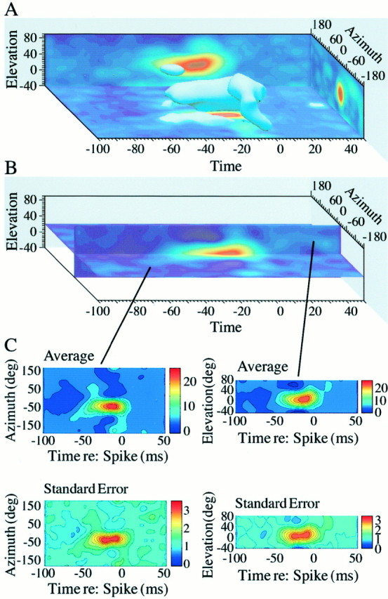
Auditory space-time receptive field estimated as a continuous function in space and time. A, Surface through this volume corresponds to an equal probability density contour. The Poisson rate λ was 10 sound events per second. This figure was derived by interpolating between measurements from the space-time kernel shown in Figure 1 and reconstructing from spiral position to spherical directions. B, Orthogonal cross-sections (one at 20° elevation and the other at −24° azimuth) taken from the receptive field of this unit. C, Bootstrapped average space-time receptive fields based on 100 resampled estimates of the space-time receptive field. Shown are the average of the 100 bootstraps and the derived SE for each position in space-time.

To assess the reliability of the estimated space-time receptive fields, we used a well known technique (Efron and Tibshirani, 1993) to bootstrap measured spike trains and obtain a sampling distribution with an average and SE. Replicates from the originally measured spike-trains were used to estimate 100 space-time receptive fields. In this analysis, cross-sectional renderings (Fig. 2B) are useful graphical displays, which can be generated for any two-dimensional plane because the modeled receptive field is continuous in both space and time. The bootstrapped average and SE for each of these cross-sections are shown in Figure 2C. The observed SE generally increases as the mean increases at each position in space-time, as expected from a Poisson process. This example illustrates that the shape of space-time receptive fields can be estimated with good confidence. A minority of neurons (23) was dropped from the database as a result of failing to demonstrate statistically reliable estimates of space receptive fields. This was typically because of insufficient spike counts.

Space-time inseparability

Space-time kernels can be classified as space-time separable or inseparable depending on whether the kernel (considered as a joint probability distribution) is equal to the outer product of its marginal distributions. In the separable case, the spatial marginal is equivalent to the static receptive field of the neuron, whereas the temporal marginal is proportional to the poststimulus time histogram. These distributions could be determined independently, and together they would nevertheless provide a complete description of the separable receptive field. In contrast, for an inseparable kernel, the outer product of the temporal and spatial marginals fails to reconstitute the kernel (Fig. 3). Features that run obliquely through a kernel are always lost when the kernel is decomposed into marginals. Oblique (or diagonal) elements are therefore a characteristic of nonseparable kernels. Such oblique patterns can be observed in the kernel shown in the cross-sectional displays of Figures4A, 5A.

Fig. 3.

Statistical tests of space-time separability. The measured space-time receptive field is plotted using ordinal position along the spiral (see Fig. 1), instead of azimuth and elevation, so that space can be treated as a single dimension. The test statistic used in this study was that of the power-divergence (PD) statistic, which unifies χ² and log-likelihood ratio. The PD statistic reflects the magnitude of the difference between the observed joint-frequency distribution f_s,τ (shown on the left) and the frequency distributionf_sf_τexpected under the assumption of independence (shown on theright):

$$PD=\frac{2}{\ell (\ell +1)}\sum _{\text{s}=1}^S \sum _{\tau =1}^T f_{\text{s},\tau }\left[{\left(\frac{f_{\text{s},\tau }}{f_{\text{s}}{f}_{\tau }}\right)}^{\ell }-1\right].$$ Equation 4

ℓ specifies membership of the power-divergence family, and in our case ℓ = 2/3 was chosen to maximize the power of the statistical test (Read and Cressie, 1988). Ncorresponds to the total number of observed output spikes. This neuron evidences a space-time inseparable kernel with a large PD statistic (PD =  23,788; df = 20,493; p < 0.01), resulting from a large difference between f_s,τ andf_s f_τ.

Fig. 4.

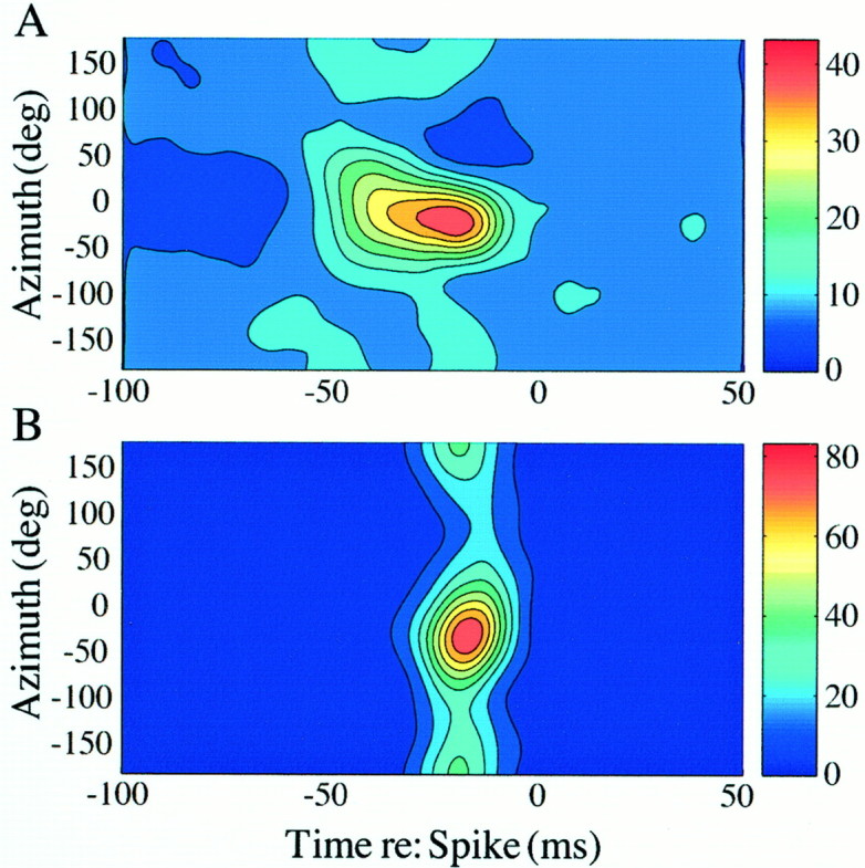
A, Inseparable (PD = 22,023; df = 20,493; p < 0.01) and B, separable (PD = 18,968; df = 20,493; p > 0.01) space-time receptive fields from two single units recorded simultaneously on the same electrode. The Poisson rate λ was 10 sound events per second.

Fig. 5.

Simulated responses to motion stimuli with sound-source trajectories of constant angular velocity along an azimuthal slice through an inseparable (A) (PD = 23,788; df = 20,493; p < 0.01), and a separable (B) (PD = 7,534; df = 20,493;p > 0.01) space-time receptive field. Theblack and red lines represent opposing directions (left-to-right vsright-to-left). The solid lines represent slower speeds, and the dotted lines represent higher speeds. The predicted instantaneous spike rates to theblack and red sound trajectories are shown in the right panels. The space-time inseparable receptive field (A) produces greater peak responses to the black compared with the redtrajectory. The separable receptive field (B) responds nearly identically to the two opposing trajectories. The receptive fields of both neurons A and B were measured with a Poisson rate λ of 20 sound events per second. The receptive field in A is the same unit also shown unwrapped in Figure 3.

Issues pertaining to separability of receptive fields have been recognized by auditory (Gerstein et al., 1968; Eggermont et al., 1981) and visual neurophysiologists (DeAngelis et al., 1995). However, formal inferential statistics were not used in these studies to test the significance of the observed inseparability of dimensions. We used the power-divergence (PD) statistic (Read and Cressie, 1988) to test the difference between observed and expected (product-of-marginals) distributions. The PD statistic is asymptotically χ² distributed with the mean equal to the degrees of freedom (df), and the variance is equal to twice the degrees of freedom. The degrees of freedom for the PD statistic are roughly equivalent to the number of space-time cells in the first-order kernel space-time matrix. When the sampling density in space and time is large, the PD statistic also asymptotically follows a normal distribution (Osius and Rojek, 1992). For example, the dimensions of space and time appear to be visually inseparable based on inspection of Figure 3. The statistical test supports this observation (PD = 23,788; df = 20,493; p < 0.01), which allows rejection of the null hypothesis that the space and time dimensions are separable. Approximately 14% (17 of 121) of AI units recorded in this study evidence significant space-time inseparability. The degree of separability of space-time receptive fields does not appear to depend either on the best frequency of the neuron or its depth within cortex, based on an examination of PD as a function of best frequency (r = −0.0579; p > 0.05) and electrode depth (r = −0.0187; p > 0.05). Additionally, in 12% of 41 positions in which two single units were recorded simultaneously on the same electrode (26 electrode penetrations), we found one of the units in the pair to be separable and the other inseparable. Figure 4 shows an example of such a discordant receptive field pairing; the PD for the unit shown in Figure4A differs significantly from the unit in Figure4B (z = 10.76; p < 0.01). Of the 36 concordant pairs, 6% were both inseparable, and 94% were both separable.

One interesting possibility is that the features of space-time receptive fields may be indicative of a tuning to the angular velocities of a moving stimulus. Figure 5(same unit as shown in spiral coordinates in Fig. 3) illustrates this by showing complementary simulated stimulus trajectories through a measured inseparable (A) and separable (B) space-time receptive field. To the right of each receptive field cross-section is shown the predicted instantaneous spike rate plotted as a function of time for each trajectory. These predicted responses are shown for several repeated passes through the receptive field with two different angular speeds (dotted vssolid) for two opposing path directions (black vsred). The steeper slope corresponds to the greater speed. In the case of the inseparable space-time receptive field, the predicted pattern of the response differs depending on the trajectory and the speed of the sound source, specifically in the peak of the response and the depth of discharge rate modulation. However, for the case of the separable space-time receptive field, there is little difference between responses for opposing path directions. Interestingly, the predicted spike rate shows less modulation for the higher speed relative to the lower speed, suggesting that although separable space-time receptive fields lack trajectory selectivity, they may nevertheless signal changes in speed. Although these simulations illustrate a possible connection between the observed pattern of the space-time receptive field and motion selectivity, it remains to be observed empirically whether these predictions hold for real sound-source movements. To test such predictions in vivorequires a quasi-real-time computation of the space-time receptive field of a neuron, a procedure that we are actively perfecting.

Evaluation of predicted responses

To demonstrate that the first-order kernel adequately estimates the space-time receptive field, the measured response trials are divided into two interleaved sets; one set is used to calculate the kernel and the other set is used to “test” the predictions of the kernel. Figure 6A shows an example of such a comparison between predicted and measured instantaneous spike rates. The predictions are generated by convolution with the first-order kernel, as described in Materials and Methods, and followed by a leaky integrator that yields the expected instantaneous rate function. Given the stochastic nature of neural responses, one cannot expect a perfect match but should nevertheless see a good degree of correlation between the measured rate function and its corresponding prediction. Indeed, the measured response is well approximated by the predicted response (r = 0.72 for the 7.5 sec response segment shown in Fig. 6A). In contrast, Figure 6B shows a control comparison between the same prediction and a different response segment that had been drawn randomly from the measured set. As expected, in this mismatched or shuffled pair, the prediction failed to capture the peaks and troughs of the measured rate function and yields a correlation coefficient near zero. Cross-correlation coefficients as a function of lag shifts are shown in Figure 6C to further quantify the similarity of the predicted to measured rate functions compared with the shuffled rate function. The cross-correlation function ensures that small phase shifts that are introduced by convolution/integration do not bias the correlation coefficient. The correlation coefficient, of course, only summarizes a linear relationship, and perhaps the addition of higher-order kernels might generate better predictions. Furthermore, the correlation coefficient as a measure of similarity is also quite sensitive to the stochastic noise present in the estimate of the first-order kernel, which will tend to deflate the correlation coefficient of the measured with the predicted response. Figure 6D provides summary box-whisker plots of correlation coefficient distributions for a subset of 12 units. Six inseparable units and six separable units were selected on the basis of having comparable kernel signal-to-noise ratios. The distribution of correlation coefficients for each unit summarizes the range of response predictability using the first-order kernel. Each correlation coefficient is based on a 7.5 sec segment over, on average, 130 segments per unit. The rate functions shown in Figure 6, Aand B, were selected from unit 4.

Fig. 6.

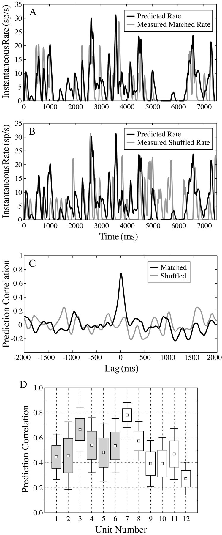
A, Predicted (black) and matched observed (gray) neural responses to spherical white-noise stimuli from an inseparable first-order kernel (prediction correlation coefficient, r = 0.72).B, Predicted (black) compared with a mismatched–shuffled observed (gray) neural response (r = 0.03). C, Cross-correlation functions of the matched (black) and shuffled (gray) predictions as a function of relative lag shifts. D, Box-whisker plots for prediction correlation coefficients for 12 units. The box reflects ±1.0 SDs, and the end-whiskers reflect ±1.96 SDs from the mean (smallsquares). Unit numbers 1–6 (grayboxes) are space-time inseparable, and unit numbers 7–12 are space-time separable. The examples shown in A–C were selected from unit 4.

DISCUSSION

White-noise methods have provided valuable tools for revealing response properties that go beyond the level of description afforded by static receptive fields (McLean et al., 1994; DeAngelis et al., 1995;Ringach et al., 1997; DiCarlo et al., 1998; Reich et al., 2000). They can also provide a method to investigate nonlinear interactions, so long as sufficient data can be collected while maintaining reliable responses from a neuron (Marmarelis and Marmarelis, 1978; Sakai, 1992;Eggermont, 1993). Of particular interest to the processing of auditory information are studies that examine spectral dynamics by constructing frequency–time (spectrotemporal) receptive fields. These used a variety of auditory stimuli, including broadband complex sounds with sinusoidal spectral profiles referred to as moving “spectral ripples” (Schreiner and Calhoun, 1994; Shamma and Versnel, 1995;Kowalski et al., 1996a,b; Klein et al., 2000), two-tones (Brosch and Schreiner, 1997), and natural sounds (Theunissen et al., 2000). However, given the evidence that implicates AI in the neural pathways responsible for the perception of sound source location, an interesting alternative to these frequency–time kernels is one that uses sound source direction, rather than sound frequency, as the independent variable in the stimulus parameter space. This was the object of the present study, and we developed a technique to estimate the shape of auditory receptive fields in two spatial (azimuth and elevation) dimensions and one temporal dimension from first-order linear kernels derived by white-noise analysis. Bootstrapping demonstrated the reliability of the receptive field estimates (Fig. 2C). Furthermore, the predictive power of the first-order kernels (Fig. 6) supports the legitimacy of these kernels in revealing the nature of the receptive field of the neuron and its space-time dynamics. The first-order kernels from some units are better than others at predicting the neural response to spherical white-noise. This could be caused by different levels of noise inherent in the kernel, although an attempt was made to select kernels with comparable signal-to-noise ratios. Alternatively, the differences in predictability may indicate differing demands for inclusion of the higher-order kernels. Given the overlap of the correlation distributions between separability conditions, there doesn't appear to be a clear distinction between the conditions in terms of the strength of first-order kernel prediction. Where one of the separable kernels (unit 7) does indeed do a remarkable job of predicting the neural response, another separable kernel (unit 12) performs rather poorly.

Using conservative quantitative inferential criteria, we produced strong evidence for the existence of a distinct subpopulation of neurons in AI showing space-time inseparability in the first-order kernel. This subpopulation represented a fairly modest proportion of neurons that we recorded in AI (∼14%). In primary visual cortex, almost 50% of neurons were reported to show space-time inseparability when the sample population was restricted to simple cells (McLean et al., 1994). Various neural mechanisms may account for the observed inseparability of dimensions, including direction-dependent adaptation and postexcitatory or inhibitory rebounds (McAlpine et al., 2000). Our method is sensitive to all of these effects, but it does not allow us to distinguish between them. In a series of simulations, we have illustrated that space-time inseparability may be indicative of the sensitivity of a neuron to the direction of sound motion (Fig. 5). Motion of a sound source is a ubiquitous feature of the acoustic environment and has stimulated both psychophysical (Middlebrooks and Green, 1991; Grantham, 1997; Perrott and Strybel, 1997; Saberi and Hafter, 1997) and neurophysiological (Altman, 1988) investigations into the neural mechanisms involved in motion processing. However, a precise definition of motion selectivity has been difficult to pin down in the auditory literature. Nevertheless, these and subsequent studies have shown that several simple aspects of sound motion are reflected in the auditory neural code (Toronchuk et al., 1992; Wagner and Takahashi, 1992; Spitzer and Semple, 1998).

The present findings do not support a strong clustering or segregation of space-time inseparable units within AI. Our sample represented only high best-frequencies (14–22 kHz) distributed unevenly among the cortical layers, and within this sample we found no evidence that space-time separability might be distributed systematically as a function of best frequency or recording depth. Furthermore, in cases in which pairs of single units were simultaneously recorded at a single electrode site, both separable and inseparable receptive fields were observed. Nevertheless, it is well known that under experimental conditions of general anesthesia, responsive neurons are found predominantly in the middle cortical layers. This was also the case in the present study in which 65% of the neurons were recorded at depths between 600 and 1200 μm. Thalamocortical projections from the ventral division of the medial geniculate body appear to produce their heaviest terminations at these depths (Huang and Winer, 2000). The strong input from this division to layers III and IV may account for the proportion of separability reported; however, the complexity of convergence to these layers may still provide the opportunity for the emergence of space-time inseparability. It is possible that inseparability is dependent on converging projections and that intrinsic projections among the other layers might yield proportions different from those observed in the middle layers. These are important considerations for further investigation, which would certainly include nonprimary auditory fields.

How successful our space-time receptive fields really are at characterizing the sensitivity of a neuron to true motion stimuli remains to be seen. If motion selectivity, as commonly defined in the vision literature (DeAngelis et al., 1995), is indeed manifest in the observed inseparability of the space and time dimensions, then our data would point to the existence of a relatively small subset of motion-sensitive neurons in AI. In any case it is well to remember that the demonstration of a preferred sound source trajectory, speed, or both does not necessarily imply that the underlying neural circuitry was constructed, or is used, solely for the purpose of auditory motion analysis. Our method does not allow us to pinpoint the mechanisms underlying the observed spatial receptive field dynamics, but it would seem most likely that these are a manifestation of the sensitivity of a neuron to dynamic changes in the binaural spectra that accompany the movement of a sound source in space.

REFERENCES

- 1.Aertsen AM, Johannesma PI. The spectro-temporal receptive field. A functional characteristic of auditory neurons. Biol Cybern. 1981;42:133–143. doi: 10.1007/BF00336731. [DOI] [PubMed] [Google Scholar]
- 2.Altman JA. Information processing concerning moving sound sources in the auditory centers and its utilization by brain integrative and motor structures. In: Syka J, Masterton RB, editors. Auditory pathway: structure and function. Plenum; New York: 1988. pp. 349–354. [Google Scholar]
- 3.Brosch M, Schreiner CE. Time course of forward masking tuning curves in cat primary auditory cortex. J Neurophysiol. 1997;77:923–943. doi: 10.1152/jn.1997.77.2.923. [DOI] [PubMed] [Google Scholar]
- 4.Brugge JF, Reale RA, Hind JE, Chan JCK, Musicant AD, Poon PWF. Simulation of free-field sound sources and its application to studies of cortical mechanisms of sound localization in the cat. Hear Res. 1994;73:67–84. doi: 10.1016/0378-5955(94)90284-4. [DOI] [PubMed] [Google Scholar]
- 5.Brugge JF, Reale RA, Hind JE. The structure of spatial receptive fields of neurons in primary auditory cortex of the cat. J Neurosci. 1996;16:4420–4437. doi: 10.1523/JNEUROSCI.16-14-04420.1996. [DOI] [PMC free article] [PubMed] [Google Scholar]
- 6.Chen J, Van Veen BD, Hecox KE. A spatial feature extraction and regularization model for the head-related transfer function. J Acoust Soc Am. 1995;1:439–452. doi: 10.1121/1.413110. [DOI] [PubMed] [Google Scholar]
- 7.DeAngelis GC, Ohzawa I, Freeman RD. Receptive-field dynamics in the central visual pathways. Trends Neurosci. 1995;18:451–458. doi: 10.1016/0166-2236(95)94496-r. [DOI] [PubMed] [Google Scholar]
- 8.deBoer E, Kuyper P. Triggered correlation. IEEE Trans Biomed Eng. 1968;15:169–179. doi: 10.1109/tbme.1968.4502561. [DOI] [PubMed] [Google Scholar]
- 9.deCharms RC, Zador A. Neural representation and the cortical code. Annu Rev Neurosci. 2000;23:613–647. doi: 10.1146/annurev.neuro.23.1.613. [DOI] [PubMed] [Google Scholar]
- 10.deCharms RC, Blake DT, Merzenich MM. Optimizing sound features for cortical neurons. Science. 1998;280:1439–1443. doi: 10.1126/science.280.5368.1439. [DOI] [PubMed] [Google Scholar]
- 11.Depireux D, Simon J, Shamma S. Measuring the dynamics of neural responses in primary auditory cortex. Theor Biol. 1998;5:89–118. [Google Scholar]
- 12.DiCarlo JJ, Johnson KO, Hsiao SS. Structure of receptive fields in area 3b of primary somatosensory cortex in the alert monkey. J Neurosci. 1998;18:2626–2645. doi: 10.1523/JNEUROSCI.18-07-02626.1998. [DOI] [PMC free article] [PubMed] [Google Scholar]
- 13.Efron B, Tibshirani RJ. An introduction to the bootstrap. Chapman and Hall; New York: 1993. [Google Scholar]
- 14.Eggermont JJ. Wiener and Volterra analyses applied to the auditory system. Hear Res. 1993;66:177–201. doi: 10.1016/0378-5955(93)90139-r. [DOI] [PubMed] [Google Scholar]
- 15.Eggermont JJ, Aertsen AM, Hermes DJ, Johannesma PI. Spectro-temporal characterization of auditory neurons: redundant or necessary. Hear Res. 1981;5:109–121. doi: 10.1016/0378-5955(81)90030-7. [DOI] [PubMed] [Google Scholar]
- 16.Eisenman LM. Neural coding of sound location: an electrophysiological study in auditory cortex using free field stimuli. Brain Res. 1974;75:203–214. doi: 10.1016/0006-8993(74)90742-2. [DOI] [PubMed] [Google Scholar]
- 17.Epping WJM, Eggermont JJ. Single-unit characteristics in the auditory midbrain of the grassfrog to temporal characteristics of sound. I. Stimulation with acoustic clicks. Hear Res. 1986;24:37–54. doi: 10.1016/0378-5955(86)90004-3. [DOI] [PubMed] [Google Scholar]
- 18.Gerstein GL, Butler RA, Erulkar SD. Excitation and inhibition in cochlear nucleus. I. Tone-burst stimulation. J Neurophysiol. 1968;31:526–536. doi: 10.1152/jn.1968.31.4.526. [DOI] [PubMed] [Google Scholar]
- 19.Grantham DW. Auditory motion perception: snapshots revisited. In: Gilkey RH, Anderson TR, editors. Binaural and spatial hearing in real and virtual environments. Erlbaum; Mahwah, NJ: 1997. pp. 295–314. [Google Scholar]
- 20.Huang CL, Winer JA. Auditory thalamocortical projections in the cat: laminar and areal patterns of input. J Comp Neurol. 2000;427:302–331. doi: 10.1002/1096-9861(20001113)427:2<302::aid-cne10>3.0.co;2-j. [DOI] [PubMed] [Google Scholar]
- 21.Imig TJ, Irons WA, Samson FR. Single-unit selectivity to azimuthal direction and sound pressure of noise bursts in cat high-frequency primary auditory cortex. J Neurophysiol. 1990;63:1448–1466. doi: 10.1152/jn.1990.63.6.1448. [DOI] [PubMed] [Google Scholar]
- 22.Jenison RL. Correlated cortical populations can enhance sound localization performance. J Acoust Soc Am. 2000;107:414–421. doi: 10.1121/1.428313. [DOI] [PubMed] [Google Scholar]
- 23.Jenison RL, Reale RA, Hind JE, Brugge JF. Modeling of auditory spatial receptive fields with spherical approximation functions. J Neurophysiol. 1998;80:2645–2656. doi: 10.1152/jn.1998.80.5.2645. [DOI] [PubMed] [Google Scholar]
- 24.Jenkins WM, Merzenich MM. Role of cat primary auditory-cortex for sound-localization behavior. J Neurophysiol. 1984;52:819–847. doi: 10.1152/jn.1984.52.5.819. [DOI] [PubMed] [Google Scholar]
- 25.Jones JP, Palmer LA. The two-dimensional spatial structure of simple receptive fields in cat striate cortex. J Neurophysiol. 1987;58:1187–1211. doi: 10.1152/jn.1987.58.6.1187. [DOI] [PubMed] [Google Scholar]
- 26.Klein DJ, Depireux DA, Simon JZ, Shamma SA. Robust spectrotemporal reverse correlation for the auditory system: optimizing stimulus design. J Comput Neurosci. 2000;9:85–111. doi: 10.1023/a:1008990412183. [DOI] [PubMed] [Google Scholar]
- 27.Kowalski N, Depireux DA, Shamma SA. Analysis of dynamic spectra in ferret primary auditory cortex. I. Characteristics of single-unit responses to moving ripple spectra. J Neurophysiol. 1996a;76:3503–3523. doi: 10.1152/jn.1996.76.5.3503. [DOI] [PubMed] [Google Scholar]
- 28.Kowalski N, Depireux DA, Shamma SA. Analysis of dynamic spectra in ferret primary auditory cortex. II. Prediction of unit responses to arbitrary dynamic spectra. J Neurophysiol. 1996b;76:3524–3534. doi: 10.1152/jn.1996.76.5.3524. [DOI] [PubMed] [Google Scholar]
- 29.Krausz HI. Identification of nonlinear systems using random impulse train inputs. Biol Cybernetics. 1975;19:217–230. [Google Scholar]
- 30.Lee YW, Schetzen M. Measurement of the Wiener kernels of a nonlinear system by cross-correlation. Int J Control. 1965;2:237–254. [Google Scholar]
- 31.Marmarelis PZ, Marmarelis VZ. Analysis of physiological systems: the white-noise approach. Plenum; New York: 1978. [Google Scholar]
- 32.Masterton RB, Imig TJ. Neural mechanisms for sound localization. Annu Rev Physiol. 1984;46:275–287. doi: 10.1146/annurev.ph.46.030184.001423. [DOI] [PubMed] [Google Scholar]
- 33.McAlpine D, Jiang D, Shackleton TM, Palmer AR. Responses of neurons in the inferior colliculus to dynamic interaural phase cues: evidence for a mechanism of binaural adaptation. J Neurophysiol. 2000;83:1356–1365. doi: 10.1152/jn.2000.83.3.1356. [DOI] [PubMed] [Google Scholar]
- 34.McLean J, Raab S, Palmer LA. Contribution of linear mechanisms to specification of local motion by simple cells in area 17 and 18 of the cat. Vis Neurosci. 1994;11:271–294. doi: 10.1017/s0952523800001632. [DOI] [PubMed] [Google Scholar]
- 35.Melssen WJ, Epping WJM. Selectivity for temporal characteristics of sound and interaural time difference of auditory midbrain neurons in the grassfrog: a system theoretical approach. Hear Res. 1992;60:178–198. doi: 10.1016/0378-5955(92)90020-n. [DOI] [PubMed] [Google Scholar]
- 36.Middlebrooks JC, Green DM. Sound localization by human listeners. Annu Rev Psychol. 1991;42:135–159. doi: 10.1146/annurev.ps.42.020191.001031. [DOI] [PubMed] [Google Scholar]
- 37.Middlebrooks JC, Pettigrew JD. Functional classes of neurons in primary auditory cortex of the cat distinguished by sensitivity to sound location. J Neurosci. 1981;1:107–120. doi: 10.1523/JNEUROSCI.01-01-00107.1981. [DOI] [PMC free article] [PubMed] [Google Scholar]
- 38.Middlebrooks JC, Clock AE, Xu L, Green DM. A panoramic code for sound location by cortical neurons. Science. 1994;264:842–844. doi: 10.1126/science.8171339. [DOI] [PubMed] [Google Scholar]
- 39.Musicant AD, Chan JCK, Hind JE. Direction-dependent spectral properties of cat external ear: new data and cross-species comparisons. J Acoust Soc Am. 1990;87:757–781. doi: 10.1121/1.399545. [DOI] [PubMed] [Google Scholar]
- 40.Osius G, Rojek D. Normal goodness-of-fit tests for multinomial models with large degrees of freedom. J Am Stat Assoc. 1992;87:1145–1152. [Google Scholar]
- 41.Perrott DR, Strybel TZ. Some observations regarding motion without direction. In: Gilkey RH, Anderson TR, editors. Binaural and spatial hearing in real and virtual environments. Erlbaum; Mahwah, NJ: 1997. pp. 275–294. [Google Scholar]
- 42.Poggio T, Girosi F. Regularization algorithms for learning that are equivalent to multilayer networks. Science. 1990;247:978–982. doi: 10.1126/science.247.4945.978. [DOI] [PubMed] [Google Scholar]
- 43.Rajan R, Aitkin LM, Irvine DR, McKay J. Azimuthal sensitivity of neurons in primary auditory cortex of cats. I. Types of sensitivity and the effects of variations in stimulus parameters. J Neurophysiol. 1990;64:872–887. doi: 10.1152/jn.1990.64.3.872. [DOI] [PubMed] [Google Scholar]
- 44.Rakhmanov EA, Saff EB, Zhou YM. Minimal discrete energy on the sphere. Math Res Lett. 1994;1:647–662. [Google Scholar]
- 45.Read TC, Cressie NAC. Goodness-of-fit statistics for discrete multivariate data. Springer; New York: 1988. [Google Scholar]
- 46.Reale RA, Chen J, Hind JE, Brugge JF. An implementation of virtual acoustic space for neurophysiological studies of directional hearing. In: Carlile S, editor. Virtual auditory space: generation and application. Landes; Georgetown, TX: 1996. pp. 153–183. [Google Scholar]
- 47.Reich DS, Mechler F, Purpura KP, Victor JD. Interspike intervals, receptive fields, and information encoding in primary visual cortex. J Neurosci. 2000;20:1964–1974. doi: 10.1523/JNEUROSCI.20-05-01964.2000. [DOI] [PMC free article] [PubMed] [Google Scholar]
- 48.Rice JJ, May BJ, Spirou GA, Young ED. Pinna-based spectral cues for sound localization in cat. Hear Res. 1992;58:132–152. doi: 10.1016/0378-5955(92)90123-5. [DOI] [PubMed] [Google Scholar]
- 49.Ringach DL, Hawken MJ, Shapley R. Dynamics of orientation tuning in macaque primary visual cortex. Nature. 1997;387:281–284. doi: 10.1038/387281a0. [DOI] [PubMed] [Google Scholar]
- 50.Saberi K, Hafter ER. Experiments on auditory motion discrimination. In: Gilkey RH, Anderson TR, editors. Binaural and spatial hearing in real and virtual environments. Erlbaum; Mahwah, NJ: 1997. pp. 315–327. [Google Scholar]
- 51.Sakai HM. White-noise analysis in neurophysiology. Physiol Rev. 1992;72:491–505. doi: 10.1152/physrev.1992.72.2.491. [DOI] [PubMed] [Google Scholar]
- 52.Schreiner CE, Calhoun BM. Spectral envelope coding in cat primary auditory cortex: properties of ripple transfer functions. Auditory Neurosci. 1994;1:39–59. [Google Scholar]
- 53.Shamma SA, Versnel H. Ripple analysis in ferret primary auditory cortex. II. Prediction of unit responses to arbitrary spectral profiles. Auditory Neurosci. 1995;1:255–270. [Google Scholar]
- 54.Spitzer MW, Semple MN. Transformation of binaural response properties in the ascending auditory pathway: influence of time-varying interaural phase disparity. J Neurophysiol. 1998;80:3062–3076. doi: 10.1152/jn.1998.80.6.3062. [DOI] [PubMed] [Google Scholar]
- 55.Theunissen FE, Sen K, Doupe AJ. Spectral-temporal receptive fields of nonlinear auditory neurons obtained using natural sounds. J Neurosci. 2000;20:2315–2331. doi: 10.1523/JNEUROSCI.20-06-02315.2000. [DOI] [PMC free article] [PubMed] [Google Scholar]
- 56.Toronchuk JM, Stumpf E, Cynader MS. Auditory cortex neurons sensitive to correlates of auditory motion: underlying mechanisms. Exp Brain Res. 1992;88:169–180. doi: 10.1007/BF02259138. [DOI] [PubMed] [Google Scholar]
- 57.Wagner H, Takahashi T. Influence of temporal cues on acoustic motion-direction sensitivity of auditory neurons in the owl. J Neurophysiol. 1992;68:2063–2076. doi: 10.1152/jn.1992.68.6.2063. [DOI] [PubMed] [Google Scholar]
- 58.Wiener N. Nonlinear problems in random theory. MIT Press; New York: 1958. [Google Scholar]
- 59.Wu Z, Chan FH, Lam FK, Chan CJ. A time domain binaural model based on spatial feature extraction for the head-related transfer function. J Acoust Soc Am. 1997;102:2211–2218. doi: 10.1121/1.419597. [DOI] [PubMed] [Google Scholar]