The Representation of Semantic Information Across Human Cerebral Cortex During Listening Versus Reading Is Invariant to Stimulus Modality

Abstract

An integral part of human language is the capacity to extract meaning from spoken and written words, but the precise relationship between brain representations of information perceived by listening versus reading is unclear. Prior neuroimaging studies have shown that semantic information in spoken language is represented in multiple regions in the human cerebral cortex, while amodal semantic information appears to be represented in a few broad brain regions. However, previous studies were too insensitive to determine whether semantic representations were shared at a fine level of detail rather than merely at a coarse scale. We used fMRI to record brain activity in two separate experiments while participants listened to or read several hours of the same narrative stories, and then created voxelwise encoding models to characterize semantic selectivity in each voxel and in each individual participant. We find that semantic tuning during listening and reading are highly correlated in most semantically selective regions of cortex, and models estimated using one modality accurately predict voxel responses in the other modality. These results suggest that the representation of language semantics is independent of the sensory modality through which the semantic information is received.

SIGNIFICANCE STATEMENT Humans can comprehend the meaning of words from both spoken and written language. It is therefore important to understand the relationship between the brain representations of spoken or written text. Here, we show that although the representation of semantic information in the human brain is quite complex, the semantic representations evoked by listening versus reading are almost identical. These results suggest that the representation of language semantics is independent of the sensory modality through which the semantic information is received.

Introduction

Humans have the unique capacity to communicate and extract meaning through both spoken and written language. Although the early sensory processing pathways for listening and reading are distinct, listeners and readers appear to extract very similar information about the meaning of a narrative story (Rubin et al., 2000; Diakidoy et al., 2005). This suggests that the human brain represents semantic information in an amodal form that is independent of input modality (Vigneau et al., 2006; Binder et al., 2009; Price, 2010, 2012). There is evidence that several cortical regions are activated during both listening and reading (for reviews, see Price, 2010, 2012). However, the demonstration of some common activation during listening and reading is necessary but not sufficient evidence of a common amodal semantic representation.

A direct and convincing way to determine if listening and reading involve a common underlying semantic representation would be to compare directly the semantic selectivity maps obtained during listening and reading of natural text, in single participants. However, to date no study has performed this crucial comparison. Most imaging studies of the semantic system have examined only one input modality, either spoken or written words (Démonet et al., 1994, 1992; Vandenberghe et al., 1996; Scott et al., 2000; Booth et al., 2002; Rissman et al., 2003; Devlin et al., 2004; Nakamura et al., 2005). Relatively few have studied cross-modal representations by presenting the same stimuli in both modalities (Petersen et al., 1989; Chee et al., 1999; Michael et al., 2001; Spitsyna et al., 2006; Jobard et al., 2007; Buchweitz et al., 2009; Liuzzi et al., 2017). Most of these cross-modality studies observed activity in left lateralized regions such as the left anterior temporal lobe, left superior temporal sulcus (STS), left middle temporal gyrus (MTG), and left inferior frontal gyrus (IFG). Most of these studies used tightly controlled stimuli, such as a set of single isolated words, sentences or curated passages, and an explicit lexical semantic task (Chee et al., 1999; Michael et al., 2001; Buchweitz et al., 2009; Liuzzi et al., 2017). A study that used narrative speech in a listening and reading task demonstrated amodal brain activity in left pSTG, left IFG, bilateral precuneus, medial prefrontal cortex (PFC), and angular gyrus (Regev et al., 2013). However, that study did not model semantic information, but only showed that voxel activations in these regions tend to be correlated across these two modalities. Furthermore, previous studies were too coarse grained to determine whether listening and reading shared semantic representations at the level of a single voxel. For example, the semantic representation of listening and reading might have been modal at a fine scale (i.e., single voxel), although amodal at a coarse scale. In sum, the evidence available currently is insufficient to determine whether semantic information obtained during listening and reading are represented in the same way.

To address this issue we used fMRI to record blood-oxygen-level-dependent (BOLD) activity in human participants while they listened to and read the same narrative stories. We then used voxelwise modeling (VM) combined with banded ridge regression (Nunez-Elizalde et al., 2019) to characterize the semantic selectivity of each voxel in each presentation modality and for each individual participant (see Materials and Methods and Naselaris et al., 2011; Nishimoto et al., 2011; Huth et al., 2012, 2016; Çukur et al., 2013; Stansbury et al., 2013; Lescroart et al., 2015). Finally, we compared the semantic tuning of each voxel in the two modalities by creating semantic maps (Huth et al., 2016) for both modalities and each individual participant. In addition, we identified modality independent cortical representation of semantic information by predicting voxel responses cross-modally. Comparison of the fit semantic models and semantic maps obtained by listening versus reading provides a sensitive and objective means to determine whether and how semantic selectivity changes depending on the modality with which semantic information is perceived.

Materials and Methods

Participants

Functional data were collected from six male participants and three female participants: S1 (male, age 31), S2 (male, age 31), S3 (female, age 28), S4 (female, age 25), S5 (male, age 30), S6 (male, age 25), and S7 (male, age 36), S8 (female, age 24), S9 (male, age 24). Two of the participants were authors on the paper (A.G.H. and A.O.N.-E.). All participants listened to and read all the stories. Listening and reading presentations were counterbalanced across participants. All participants were healthy and had normal hearing, and normal or corrected-to-normal vision. One participant was left handed, all other participants were right handed or ambidextrous according to the Edinburgh handedness inventory (Oldfield, 1971) (laterality quotient of −100: entirely left-handed, +100: entirely right-handed). Laterality scores were +90 (decile R.7), +70 (decile R.3), +10 (ambidextrous), +80 (decile R.5), +80 (decile R.5), +80 (decile R.5), −60 (decile L.3), +90 (decile R.7) and +95 (decile R.9) for S1–9, respectively. To stabilize head motion during scanning sessions participants wore a personalized head case that precisely fit the shape of each participant's head (https://caseforge.co/).

Natural speech stimuli

The speech stimuli consisted of 10- to 15 min stories taken from The Moth Radio Hour and used previously (Huth et al., 2016). In each story, a speaker tells an autobiographical story in front of a live audience. The 10 selected stories cover a wide range of topics and are highly engaging. The model validation dataset consisted of one 10 min story. This story was played twice for each participant (once during each scanning session), and then the two responses were averaged (for details, see Huth et al., 2016).

Speech stimuli were played over Sensimetrics S14 in-ear piezoelectric headphones (Sensimetrics). A Behringer Ultra-Curve Pro hardware parametric equalizer was used to flatten the frequency response of the headphones based on calibration data provided by Sensimetrics. All stimuli were played at 44.1 kHz using the pygame library in Python. All stimuli were normalized to have peak loudness of −1 dB relative to max. However, the stories were performed by different speakers and were not uniformly mastered, so some differences in total loudness remain.

Story transcription and preprocessing

Each story was manually transcribed by one listener, and this transcription was checked by a second listener. Certain sounds (e.g., laughter, lip-smacking and breathing) were also marked to improve the accuracy of the automated alignment. The audio of each story was down-sampled to 11.5 kHz and the Penn Phonetics Lab Forced Aligner (P2FA; Yuan and Liberman, 2008) was used to automatically align the audio to the transcript. The forced aligner uses a phonetic hidden Markov model to find the temporal onset and offset of each word and phoneme. The Carnegie Mellon University pronouncing dictionary was used to guess the pronunciation of each word. The Arpabet phonetic notation was used when necessary to manually add words and word fragments that appeared in the transcript but not in the dictionary.

After automatic alignment was complete, Praat (Boersma and Weenink, 2001) was used to check and correct each aligned transcript manually. The corrected aligned transcript was then spot-checked for accuracy by a different listener.

Finally the aligned transcripts were converted into separate word and phoneme representations using Praat's TextGrid object. The phoneme representation of each story is a list of pairs (P, t), where P is a phoneme and t is the onset time in seconds. Similarly the word representation of each story is a list of pairs (W, t), where W is a word and t is the onset time in seconds.

Natural reading stimuli

The same stories from listening sessions were used for reading sessions. Praat's word representation for each story (W, t) was used for generating the reading stimuli. The words of each story were presented one-by-one at the center of the screen using a rapid serial visual presentation (RSVP) procedure (Forster, 1970; Buchweitz et al., 2009). During reading, each word was presented for a duration precisely equal to the duration of that word in the spoken story. RSVP reading is different than natural reading because during RSVP the reader has no control over which word to read at each point in time. Therefore, to make listening and reading more comparable we matched the timing of the words presented during RSVP to the rate at which the words occurred during listening.

The pygame library in Python was used to display text on a gray background at 34 horizontal, and 27 vertical degrees of visual angle. Black letters were presented at average 6 (min = 1, max = 16) horizontal and 3 vertical degrees of visual angle. A white fixation cross was present at the center of the display. Participants were asked to fixate while reading the text. These data were collected during two 3 h scanning sessions that were performed on different days. Participants' eye movement were monitored at 60 Hz throughout the scanning sessions using a custom-built camera system equipped with an infrared source (Avotec) and the ViewPoint EyeTracker software suite (Arrington Research). The eye tracker was calibrated before the first run of data acquisition. Certain auditory sounds (laughter and applause) were presented as text to provide cues about the ambiance of each story.

Semantic model construction

To account for response variance caused by the semantic content of the story stimuli a 985-parameter semantic feature space based on word co-occurrence statistics in a large corpus of text (Deerwester et al., 1990; Lund and Burgess, 1996; Mitchell et al., 2008; Huth et al., 2016) was used. In short, a word co-occurrence matrix, M, with 985 rows and 10,470 columns was created. The 985 rows describe 985 basic words from Wikipedia's List of 1000 Basic Words, the 10,470 columns are words selected from a very large corpora of 13 transcripts of Moth stories (including the 10 used as stimuli in the experiments described in this paper), 604 popular books available through Project Guttenberg, 2,405,569 Wikipedia pages, 36,333,459 reddit.com user comments (for a detailed description, see Huth et al., 2016).

Iterating through the text corpus, we added 1 to M_i,j each time word j appeared within 15 words of basis word i. Once the word co-occurrence matrix was complete, we log-transformed the counts, replacing M_i,j with log(1 + M_i,j). Next, each row of M was z-scored to correct for differences in basis word frequency, and then each column of M was z-scored to correct for word frequency. Each column of M is now a 985-dimensional semantic vector representing one word in the lexicon.

The semantic model stimulus matrix was then constructed from the stories: for each word-time pair (w, t), within each story the corresponding column of M was selected, creating a new list of semantic vector-time pairs, (M_w,t). These unevenly sampled lists of vectors were resampled at times corresponding to the fMRI acquisitions using a three-lobe Lanczos filter with the cutoff frequency set to the Nyquist frequency of the fMRI acquisition (0.249 Hz).

Motion-energy model construction

A spatiotemporal Gabor pyramid was used to extract low-level visual features from the sequence of word frames used in the reading experiment (Adelson and Bergen, 1985; Watson and Ahumada, 1985). The word frames were first cropped to 400 × 400 pixels (14 horizontal, and 14 vertical degrees of visual angle) to include mainly the words and then down-sampled to 96 × 96 pixels to minimize computational cost. The word frames were then converted to the CIE L*A*B* color space (McLaren, 1976) and the color information was discarded. The spatiotemporal Gabor pyramid consisted of a total of 39 three-dimensional Gabor filter pairs of orthogonal quadrature spanning a square grid that covered the screen. The filters consisted of two spatial and one temporal dimension and were created using five spatial frequencies (0, 2, 4, 6, and 8 cycles/image), three temporal frequencies (0, 2 and 4 Hz), and four directions of motion (0, 90, 180, and 270 degrees). Each of the filters was convolved with the sequence of word frames. The resulting filter activations were squared and summed for each quadrature pair, resulting in a 39-dimensional feature vector for each word frame. The output was down-sampled to the functional image acquisition rate (2.0045 s) using sinc interpolation (Oliphant, 2007). For more details, see Nishimoto et al. (2011). However, note that only five spatial frequencies and four directions of motion were used here.

Spectral model construction

A cochleogram model that accounts for the logarithmic filtering of the mammalian coclea described in (de Heer et al., 2017) was used to create the low level auditory features (80 parameters). This model was selected based on an earlier study showing that it outperforms other low level acoustical models (de Heer et al., 2017). The 80 waveforms of the coclear filter bank were between 264 and 7360 Hz, spaced at 25% of the bandwidth. The spectral features were down-sampled to the rate of acquisition of the functional images (2.0045 s) using a Lanczos filter.

Syntax model construction

The syntactic properties of each spoken word were labeled. A pretrained neural network was used to create a parse tree for each sentence of the stories (Andor et al., 2016). Two feature spaces were extracted from the parse trees. The first was constructed from the part-of-speech tags (e.g., noun, verb) by assigning a value of one to each entry in which the part-of-speech tag appeared and all other entries were set to zero (12 parameters). The second feature space captured the word dependencies in the sentence (i.e., direct object, indirect object, etc.) and was constructed by assigning a value of one to each entry in which the word dependency appeared and all other entries were set to zero (44 parameters). For each syntactic feature (e.g., noun), a time course was created with a value of 1 whenever a word was labeled with that feature and 0 otherwise. The syntactic features were then down-sampled to the rate of acquisition of the functional images (2.0045 s) using a Lanczos filter.

Phoneme model construction

To account for response variance caused by the low-level phonemic content of the stories, a 39-parameter model that captures how often each of the 39 phonemes in English was spoken over time was constructed. The phoneme representations of the stories were used to construct this model: the lists of phoneme–time pairs (P, t) were rearranged into 39 lists, each of which contains only the times of a single phoneme. These lists of times were then down-sampled to the fMRI acquisition rate (2.0045 s).

Letter model construction

To account for response variance caused by the letters during reading a 26-parameter model that captures how often each of the 26 letters in English was present on screen over time was constructed. This was constructed by counting the number of times a letter was present within a word and then down-sampled to the fMRI acquisition rate (2.0045 s).

Word rate, word length variation, phoneme rate, letter rate, and pauses model construction

To account for the highly variable speech rate both within and across stories, single-feature models that simply count the number of words, number of phonemes, number of letters, and number of story speaker's pauses that occurred during the acquisition of each fMRI volume (2.0045 s) were constructed. To account for the variable word lengths during the visual presentation a single-feature word length variation model was constructed by taking the variance of word lengths that occurred during the acquisition of each fMRI volume.

Stimulus down-sampling

Before down-sampling to the fMRI acquisition rate, the phoneme and semantic models were represented as unevenly sampled impulse trains. A three-lobe Lanczos filter with cutoff frequency set to the fMRI Nyquist rate (0.249 Hz) was used to resample these impulse trains at evenly spaced time points corresponding to the middle of each fMRI volume.

Experimental design and statistical analysis

fMRI data acquisition.

Each spoken and written story was presented during a separate fMRI scan. The length of each scan was the same as the story. Each scan included 10 s (5 TR) of silence both before and after the story. These data were collected during 2 3 h scanning sessions that were performed on different days.

MRI data were collected on a 3T Siemens TIM Trio scanner at the UC Berkeley Brain Imaging Center using a 32-channel Siemens volume coil. Functional scans were collected using gradient echo EPI water excitation pulse sequence with repetition time (TR) = 2.0045 s, echo time (TE) = 31 ms, flip angle = 70 degrees, voxel size = 2.24 × 2.24 × 4.1 mm (slice thickness = 3.5 mm with 18% slice gap), matrix size = 100 × 100, and field of view = 224 × 224 mm. 30 axial slices were prescribed to cover the entire cortex and were scanned in interleaved order. A custom-modified bipolar water excitation radiofrequency (RF) pulse was used to avoid signal from fat. Anatomical data were collected using a T1-weighted multi-echo MP-RAGE sequence on the same 3T scanner.

fMRI data pre-processing.

Each functional run was motion-corrected using the FMRIB Linear Image Registration Tool (FLIRT) from FSL 5.0 (Jenkinson and Smith, 2001; Jenkinson et al., 2002). All volumes in the run were then averaged across time to obtain a high quality template volume. FLIRT was also used to automatically align the template volume for each run to the overall template, which was chosen to be the temporal average of the first functional run for each participant. The temporal averages of the cross-modal runs (listening or reading) were also automatically aligned to the same overall template. These automatic alignments were manually checked and adjusted as necessary to improve accuracy. The cross-run transformation matrix was then concatenated to the motion-correction transformation matrices obtained using MCFLIRT, and the concatenated transformation was used to resample the original data directly into the overall template space.

Low-frequency voxel response drift was identified using a third order Savitsky–Golay filter with a 120 s window. This drift was subtracted from the signal. Responses of each story were z-scored separately; that is, the mean response for each voxel was subtracted and the remaining response was scaled to have unit variance. Before the VM, 10 TRs from the beginning and 10 TRs at the end of each story were discarded.

Cortical surface reconstruction and visualization

Cortical surface meshes were generated from the T1-weighted anatomical scans using Freesurfer software (Dale et al., 1999). Before surface reconstruction, anatomical surface segmentations were carefully hand-checked and corrected using Blender software and pycortex (Gao et al., 2015) (http://pycortex.org). Relaxation cuts were made into the surface of each hemisphere. Blender and pycortex were used to remove the surface crossing the corpus callosum. The calcarine sulcus cut was made at the horizontal meridian in V1 using retinotopic mapping data as a guide.

Functional images were aligned to the cortical surface using pycortex. Functional data were projected onto the surface for visualization and analysis using the line-nearest scheme in pycortex. This projection scheme samples the functional data at 64 evenly spaced intervals between the inner (white matter) and outer (pial) surfaces of the cortex and then averages together the samples. Samples are taken using nearest-neighbor interpolation, wherein each sample is given the value of its enclosing voxel.

Localizers for known ROIs

Known ROIs were localized separately in each participant using standard techniques (Spiridon et al., 2006; Hansen et al., 2007). For all participants, ROIs were defined using three experiments: a visual category localizer, an auditory cortex (AC) localizer, and a motor localizer. For some participants retinotopic visual ROIs using a retinotopic localizer and area MT+ using an MT localizer were defined.

Visual category localizer.

Visual category localizer data were collected in six 4.5 min scans consisting of 16 blocks, each 16 s long. During each block, 20 images of places, faces, human body parts, nonhuman animals, household objects, or spatially scrambled household objects were displayed. Each image was displayed for 300 ms followed by a 500 ms blank. Occasionally, the same image was displayed twice in a row, in which case the participant was asked to respond with a button press.

The contrast between faces and objects was used to define the fusiform face area (Kanwisher et al., 1997) and occipital face area (Halgren et al., 1999). The contrast between human body parts and objects was used to define the extrastriate body area (Downing et al., 2001). The contrast between places and objects was used to define the parahippocampal place area (Epstein and Kanwisher, 1998), occipital place area (Nakamura et al., 2000), and retrosplenial cortex.

Auditory cortex localizer.

AC localizer data were collected in one 10 min scan. The participant listened to 10 repeats of a 1 min auditory stimulus, which consisted of 20 s segments of music (Arcade Fire), speech (Ira Glass), and natural sound (a babbling brook). To determine whether a voxel was responsive to auditory stimuli, the repeatability of the voxel response across the 10 stimulus repeats was calculated using an F-statistic. The F-statistic map was used to define the auditory cortex (AC).

Motor localizer.

Motor localizer data were collected during one 10 min scan. The participant was cued to perform six different motor tasks in a random order in 20 s blocks. For the hand, mouth, foot, speech, and rest blocks the stimulus was simply a word at the center of the screen (e.g., “Hand”). For the saccade block, the participant was shown a pattern of saccade targets.

For the “Hand” cue, the participant was instructed to make small finger-drumming movements with both hands for as long as the cue remained on the screen. Similarly for the “Foot” cue the participant was instructed to make small toe movements for the duration of the cue. For the “Mouth” cue, the participant was instructed to make small mouth movements approximating the nonsense syllables balabalabala for the duration of the cue—this requires movement of the lips, tongue, and jaw. For the “Speak” cue, the participant was instructed to continuously subvocalize self-generated sentences for the duration of the cue. For the saccade condition the written cue was replaced with a fixed pattern of 12 saccade targets, and the participant was instructed to make frequent saccades between the targets. A linear model was used to find the change in BOLD response of each voxel in each condition relative to the mean BOLD response.

Weight maps for the foot, hand, and mouth responses were used to define primary motor and somatosensory areas for the feet (M1F, S1F), hands (M1H, S1H), and mouth (M1M, S1M); supplementary motor areas for the feet and hands; secondary somatosensory area for the feet, and, in some participants, the hands; and, in some participants, the ventral premotor hand area (Penfield and Boldrey, 1937). The weight map for saccade responses was used to define the frontal eye field (Paus, 1996), frontal operculum eye movement area (Corbetta et al., 1998), intraparietal sulcus visual areas, and, in some participants, the supplementary eye field (Grosbras et al., 1999). The weight map for speech production responses was used to define Broca's area (Amunts et al., 2010; Zilles and Amunts, 2018) and the superior ventral premotor speech area (sPMv).

Retinotopic localizer.

Retinotopic mapping data were collected in four 9 min scans. Two scans used clockwise and counterclockwise rotating polar wedges, and two used expanding and contracting rings. Visual angle and eccentricity maps were used to define visual areas V1, V2, V3, V4, LO, V3A, V3B, and V7 (Hansen et al., 2007).

Area MT+ localizer.

Area MT+ localizer data were collected in four 90 s scans consisting of alternating 16 s blocks of continuous and temporally scrambled natural movies. The contrast between continuous and temporally scrambled natural movies was used to define visual motion area MT+ (Tootell et al., 1995).

Voxelwise model fitting

A single joint model that included all feature spaces was estimated for each voxel in each dataset (listening and reading) separately using banded ridge regression (for details, see below and Nunez-Elizalde et al., 2019). Banded ridge regression assigns a different regularization parameter for every feature space and so reduces bias caused by correlations between feature spaces.

Feature spaces

The feature spaces were motion-energy features (39 parameters), spectral features (80 parameters), word rate (1 parameter), phoneme rate (1 parameter), phonemes (39 parameters), letter rate (1 parameter), letters (26 parameters), word length variation per repetition time (1 parameter), syntactic features (56 parameters), and co-occurrence semantics (985 parameters). The motion-energy, spectral, word rate, phoneme rate, phonemes, letter rate, letters, and word length variation features were used to explain away low-level parameters that might otherwise contaminate the semantic model weights.

Before doing regression, each feature channel was z-scored within each story (training and testing features were z-scored independently) by subtracting the mean and dividing by the standard deviation. This was done to match the features to the fMRI responses, which were also z-scored within each story. In addition, 10 TRs from the beginning and 10 TRs at the end of each story were discarded before VM.

Banded ridge regression

We combine several feature spaces in the VM approach. To assign different levels of regularization to each feature space, we estimate all our models simultaneously using banded ridge regression (Nunez-Elizalde et al., 2019). Under banded ridge regression, brain responses are modeled as a linear combination of all the feature spaces. However, each feature space is assigned a different value of the regularization parameter. Banded ridge regression is a special case of the well-established statistical approach called Tikhonov regression (Tikhonov and Arsenin, 1977). The solution to the Tikhonov regression problem is given by β̂ = argmin_β[‖Y − Xβ‖₂² + ‖λCβ‖₂²], where C is the penalty matrix. In case of banded ridge regression, the matrix C is a diagonal matrix whose entries correspond to the regularization levels appropriate for each feature space. To find the optimal regularization parameter for every feature space a wide range of regularization parameters is explored using cross-validation. The regularization parameter is optimized based on prediction accuracy on a held-out dataset. Note that in case of λ = 0 Tikhonov regression reduces to the ordinary least squares and in case of C = I Tikhonov regression reduces to ridge regression.

BOLD responses were modeled as a linear combination of all the feature spaces using linear regression with a non-spherical spatiotemporal multivariate normal prior on the weights (Nunez-Elizalde et al., 2019). This approach allows us to impose different levels of regularization on each feature space within the joint model for each voxel, which is important because of differences in feature space size and signal-to-noise levels. The regularization parameter for each feature space was estimated empirically via cross-validation on a held-out set.

Within the same model, the hemodynamic response function was modeled using a finite impulse response (FIR) filter per voxel and for each subject and modality (listening and reading) separately. This was implemented by modeling the BOLD responses at 10 temporal delays corresponding to 0, 2, 4, 6, … 16, and 18 s. We also imposed a multivariate normal prior on the temporal covariance of the FIR filter. The temporal prior was constructed from a set of HRF basis functions (Penny et al., 2007).

Cross-validation

We used cross-validation to find the optimal regularization parameter for each feature space in the joint model. Because evaluating k regularization parameters for m models leads to k^m combinations, conducting a grid-search in our high-dimensional parameter space is impractical (requiring 10¹⁰ model fits). To overcome this problem, we used a tree-structured Parzen search (Bergstra et al., 2011). We performed the search 25 times each time using different initialization values and stopped each search after 300 iterations. For every set of regularization parameters tested in each iteration, we performed fivefold cross-validation twice. We used the coefficient of determination (R²) between the predicted and the actual voxel responses as our performance metric for each validation fold.

Model estimation and evaluation

We computed the mean prediction performance across cross-validation folds per voxel for each of the 7500 (300 × 25) regularization parameter sets tested. The regularization parameters that yielded the maximum cross-validated prediction performance were selected for each voxel. These regularization parameters were then used to estimate the model weights for each of the voxels in each modality independently for each of the nine subjects.

To validate the voxelwise models, estimated model weights were used to predict responses to a validation story that was not used for model estimation. Only the estimated semantic model weights were used for model predictions. Pearson's correlation coefficient was computed between the predicted responses and the mean of the two validation datasets (291 time points).

Statistical significance was computed by a permutation test with 10,000 iterations and comparing estimated correlations to the empirical null distribution of correlations for each participant and modality separately. At each permutation iteration, the time course of the held-out validation dataset was permuted by blockwise shuffling (10 TRs were blocked to account for autocorrelations in voxel responses), and then Pearson's correlation coefficient between the permuted voxel response and the predicted voxel response was computed for each voxel separately. This produced a distribution of 10,000 estimates of correlation coefficients for each voxel, participant, and modality. These 10,000 estimates define an empirical distribution that was used to obtain a p-value. Resulting p-values were corrected for multiple comparisons within each participant using the false discovery rate (FDR) procedure (Benjamini and Hochberg, 1995).

Voxelwise model fitting and analysis was performed using custom software tikreg (Nunez-Elizalde et al., 2019) written in Python, making heavy use of NumPy (Oliphant, 2006) and SciPy (Oliphant, 2007). Analysis and visualizations were developed using iPython (Pérez and Granger, 2007) and the interactive programming and visualization environment jupyter notebook (Kluyver et al., 2016).

Semantic PC projections

Listening model weights and reading model weights were projected onto the semantic subspace that was created in a previous study from our laboratory (Huth et al., 2016). That study recovered a low-dimensional semantic subspace from an aggregated set of estimated semantic model weights using principal components analysis. Taking the dot product of the estimated model weights with the low-dimensional semantic subspace revealed for each voxel a projection along the 985 semantic principal components (PCs). To visualize which semantic concepts are represented in each voxel we used an RGB color space to map the first three semantic PC projections onto the cortical surface separately for the two modalities (Huth et al., 2012, 2016).

Correlating the semantic principal components

Pearson's correlation coefficient was computed between each semantic projection in listening and the corresponding semantic projection in reading. To find out whether the semantic projections could be correlated by chance, a permutation test with 10,000 iterations was performed for each individual participant separately. The correlation was computed for the 10,000 best predicted voxels by the co-occurrence semantics model in both modalities. The best predicted voxels were selected by taking an average of listening and reading model prediction accuracies per voxel and selecting the 10,000 voxels with highest mean predictions. At each permutation iteration, (1) the time courses of the feature matrix was permuted (note that the feature matrix is the same for listening and reading sessions), (2) banded ridge regression was performed between the fMRI responses and this permuted matrix, (3) the estimated model weights were projected onto the semantic principal component space, and (4) Pearson's correlation coefficient between projections of the listening and reading weights onto the semantic subspace were computed separately for each PC. This results in a distribution of 10,000 estimates of correlation coefficients for each semantic PC and participant. Statistical significance was defined as any correlation coefficient that exceeded 95% of all of the permuted correlations.

Cross-modality voxelwise model fitting

Estimated model weights (see “Voxelwise model fitting”) from one modality (e.g., listening) were used to predict voxel responses in the other modality (e.g., reading). Model prediction accuracy was then computed using Pearson's correlation coefficient between cross-modal prediction responses (e.g., listening model estimates predicting reading responses) and the mean of the two validation responses (e.g., reading responses).

Results

We sought to determine whether and how the cortical representation of semantic information in narrative language might depend on the modality with which it is perceived. Nine participants listened to and read narrative stories while whole-brain BOLD activity were recorded by means of functional MRI (Fig. 1). The experimental stimuli consisted of more than two hours of narrative stories from The Moth Radio Hour, along with written transcriptions of the same stories. In the reading condition we used an RSVP method (Forster, 1970; Buchweitz et al., 2009) to present the stories at precisely the same rate as they occurred during listening. That is, in the reading condition each word was presented serially at exactly the same time, and for exactly the same duration as when it was spoken. The semantic content of the stories was estimated continuously by projecting the narrative into a word embedding space based on word co-occurrence statistics (Church and Hanks, 1990; Lund and Burgess, 1996; Mitchell et al., 2008; Turney and Pantel, 2010; Wehbe et al., 2014). We then used VM to estimate a set of weights for each voxel that best characterize the relationship between the semantic features and the recorded BOLD signals separately for each modality. These estimated model weights were then used to predict voxel responses in a held-out validation dataset both within and across modalities. Finally, the semantic tuning of each voxel in the two modalities was compared by projecting the estimated model weights onto the semantic space described in Huth et al. (2016).

Figure 1.

Experimental procedure and VM. Nine participants listened to and read over two hours of natural stories in each modality while BOLD responses were measured using fMRI. The presentation time of single words was matched between listening and reading sessions. Semantic features were constructed by projecting each word in the stories into a 985-dimensional word embedding space independently constructed using word co-occurrence statistics from a large corpus. These features and BOLD responses were used to estimate a separate FIR banded ridge regression model for each voxel in every individual participant. These estimated model weights were used to predict BOLD responses for a separate held-out story that was not used for model estimation. Predictions for individual participants were computed separately for listening and reading sessions. Model performance was quantified as the correlation between the predicted and recorded BOLD responses to this held-out story. Within-modality prediction accuracy was quantified by correlating the predicted responses from one modality (e.g., listening) with the recorded responses to the same modality (e.g., listening). Cross-modality prediction accuracy was quantified by correlating the predicted responses for one modality (e.g., listening) with the recorded responses of the other modality (e.g., reading).

Does the cortical distribution of semantically selective voxels depend on stimulus modality?

We used a VM procedure to determine whether the broad distribution of semantically selective voxels depends on presentation modality. Semantic features were extracted from the stories and these were used to estimate voxelwise model weights for BOLD signals that were recorded while participants listened to the stories in the training set. These estimated model weights were then used to predict fMRI voxel responses to a separate held-out validation set. We repeated the same procedure for the reading sessions. Several low-level features (low-level visual, spectral, word rate, letter rate, word length variation, phonemes, phoneme rate, and pauses) and syntactic features were included alongside the semantic features as nuisance regressors (see Materials and Methods), but these nuisance regressors were discarded after regression and the final model predictions were based only on semantic model weight estimates. The correlation coefficient between the actual responses in the held-out validation dataset and predicted responses were computed to give a measure of model prediction accuracy. These were then mapped onto the cortical surface.

Figure 2 shows voxelwise model prediction accuracy for listening and reading for all voxels in one participant (p < 0.05, FDR corrected). Figure 2a shows that our semantic model predicts brain activity in a broadly distributed semantic system when participants listen to natural stories, replicating our previous study (Huth et al., 2016). This system extends across much of lateral temporal cortex (LTC), ventral temporal cortex (VTC), lateral parietal cortex (LPC), medial parietal cortex (MPC), medial PFC, superior PFC, and inferior PFC. Figure 2b shows that when participants read natural stories this network of brain regions are similarly well predicted by the semantic model. Figure 2c compares prediction accuracy of semantic models fit to listening (depicted on the x-axis) versus reading (depicted on the y-axis). The saturation of each point represents the number of voxels that fall into a given range of prediction accuracy. Most voxels are approximately equally well predicted in both modalities. Overall, the semantic model accurately predicts activity in most of the semantic system independent of the presentation modality.

Figure 2.

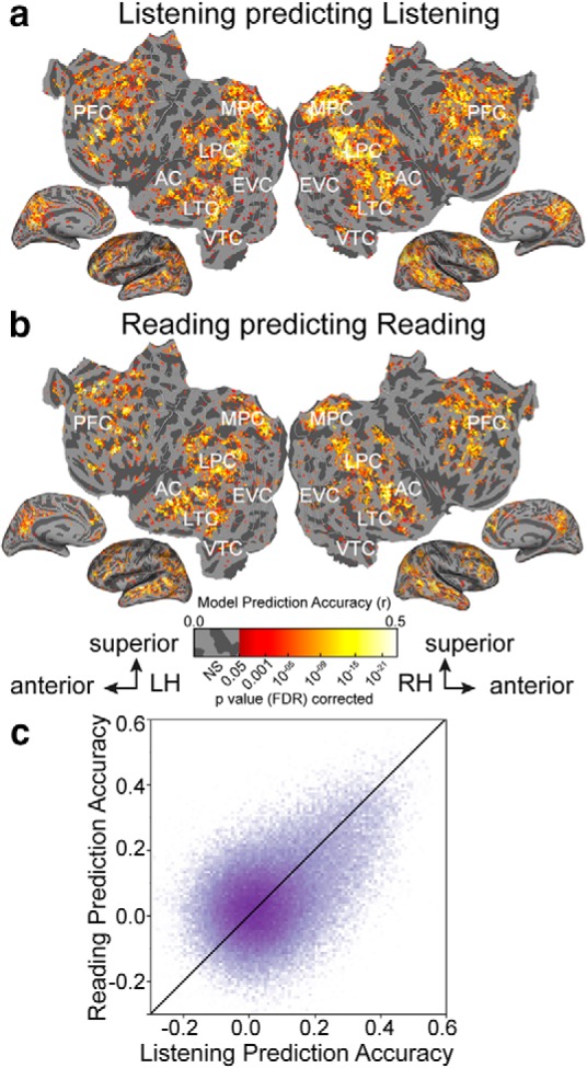
Semantic model prediction accuracy across the cortical surface. VM was used to estimate semantic model weights in two modalities, listening and reading. Prediction accuracy was computed as the correlation (r) between the participant's recorded BOLD activity to the held-out validation story and the responses predicted by the semantic model. a, Accuracy of voxelwise models estimated using listening data and predicting withheld listening data. The flattened cortical surface of one participant is shown. Prediction accuracy is given by the color scale shown at bottom. Voxels that are well predicted appear yellow or white, voxel predictions that are not statistically significant are shown in gray (p > 0.05, FDR corrected; LH, left hemisphere; RH, right hemisphere; NS, not significant; EVC, early visual cortex). b, Accuracy of voxelwise models estimated using reading data and predicting withheld reading data. The format is the same as in a. Estimated semantic model weights accurately predict BOLD responses in many brain regions in the semantic system, including LTC, VTC, LPC, MPC, and PFC in both modalities. In contrast, voxels in the early sensory regions such as the primary AC and early visual cortex are not well predicted. c, Log transformed density plot of the listening (x-axis) versus reading (y-axis) model prediction accuracy. Purple points indicate all voxels. Darker colors indicate a higher number of voxels in the corresponding bin. Voxels with listening prediction accuracy <0.17 and reading prediction accuracy <0.19 are not significant. Most voxels are equally well predicted in listening and reading indicating that these voxels represent semantic information independent of the presentation modality.

Figure 3 shows voxelwise model prediction accuracy for listening and reading for all voxels and across nine participants in the standard MNI brain space. Figure 3, a and b, show average prediction accuracy across all participants in listening and reading, respectively. Figure 3, c and d, show for each voxel the number of participants where semantic model prediction accuracy is significant in listening and reading, respectively. These results show that our semantic model predicts brain activity within the semantic system in all participants. However, due to averaging across participants voxel prediction accuracies are lower than in individual participant results (maximum prediction accuracy across all MNI voxels for listening 0.27 ± 0.03, maximum prediction accuracy across all MNI voxels for reading: 0.28 ± 0.03).

Figure 3.

Semantic model prediction accuracy across all participants in standard brain space. VM was used to assess semantic model prediction accuracy in the listening and reading modalities for all nine participants as described in Figure 2, a and b. Prediction accuracies computed in individual subject's space were then projected into a standard MNI brain space. a, Average listening prediction accuracy across nine participants was computed for each MNI voxel in the standard brain space and is mapped onto the cortical surface of the MNI brain. Average prediction accuracy is given by the color scale. Voxels that are well predicted appear brighter. Across all participants the estimated semantic model weights in the listening modality accurately predict BOLD responses in many brain regions in the semantic system, including LTC, VTC, LPC, MPC, and PFC. (LH, Left hemisphere, RH: Right hemisphere, EVC, early visual cortex). b, Average reading prediction accuracy across nine participants was computed for each MNI voxel in the standard brain space and is mapped onto the cortical surface of the MNI brain. The format is the same as in a. Across all participants, estimated semantic model weights in the reading modality accurately predict BOLD responses in the semantic system. c, Significant prediction accuracy in each voxel in the listening modality was determined in the subject space and then projected to the standard MNI brain space. The number of subjects with significant semantic model prediction accuracy for a given MNI voxel is then mapped onto the cortical surface of the MNI brain. Number of participants is given by the color scale shown at bottom. Dark red voxels are significantly well predicted in all participants. Dark blue voxels are not significantly predicted in any participant. d, Significant prediction accuracy in each voxel in the reading modality was determined in the subject space and then projected to the standard MNI brain space. The number of subjects with significant semantic model prediction accuracy for a given MNI voxel is then mapped onto the cortical surface of the MNI brain. The format is the same as in c. Most of the voxels in the semantic system are significantly predicted by all participants in both modalities.

Does the representation of semantic information vary with sensory modality?

To determine whether semantic representation is modality independent we compared the semantic tuning of each voxel estimated during listening versus reading. The semantic tuning of each voxel is given by a 985-dimensional vector of weights, one weight for each of the 985 semantic features. Because there are ∼80,000 cortical voxels in each individual participant and 985 semantic features it is impractical to make comprehensive comparisons for each feature. Therefore, to simplify interpretation the estimated semantic model weights were projected into a low-dimensional semantic subspace that captures most of the information about the semantic selectivity of the voxel population. This semantic subspace was created by applying principal component analysis to an aggregated set of estimated semantic model weights from seven participants included in a previous study from our laboratory (Huth et al., 2016). (Note that three of those who participated in the earlier study are also included in the current study.) The resulting semantic principal components (PCs) are ordered by how much variance they explain across the voxels. By projecting both the listening model weights and the reading model weights separately into these semantic PCs, we ensure that cortical voxels that represent similar concepts will project to nearby points in the semantic space.

To visualize which semantic concepts are represented in each voxel, we mapped the projections of the first three semantic principal components onto each participant's cortical surface separately for the two modalities. Each voxel was then colored according to a simple RGB color scheme, where the color red represents the first semantic PC, the color green represents the second semantic PC, and blue the third semantic PC. Inspection of the listening and reading semantic maps shown in Figure 4 reveals that the semantic representations in both modalities are very similar. The similarity between the listening and reading semantic maps indicate that individual voxels within the semantic system are tuned for the same semantic concepts regardless of presentation modality.

Figure 4.

Semantic tuning maps for listening and reading. The semantic maps for both modalities are displayed on the cortical surface of one participant. a, Voxelwise model weights for the listening sessions were projected into a semantic space created by performing principal component analysis on estimated semantic model weights acquired during a listening experiment published earlier (Huth et al., 2016). Each voxel is colored according to its projection onto the first (red), second (blue) or third (green) semantic PC. The color wheel legend at center indicates the associated semantic concepts. Voxels whose within-modality prediction was not statistically significant are shown in gray (p > 0.05, FDR corrected; LH, left hemisphere; RH, right hemisphere; EVC, early visual cortex). b, Voxelwise model weights for the reading sessions projected into the semantic space, and colored using the same procedure as in a. Comparison of panels a and b reveals that semantically selective voxels are tuned for similar semantic concepts during both listening and reading.

To quantify the similarity between the semantic maps shown in Figure 4 for all participants, we correlated the projections of the listening and reading model weights into the semantic PCs across the two modalities (listening and reading). To reduce noise, the 10,000 voxels that were best predicted by the semantic model in the two modalities were selected for this analysis. The listening and reading semantic PC projections were then correlated for each semantic PC separately.

Figure 5 shows these correlation coefficients for the first 10 semantic PC projections and for all nine participants. Each colored diamond shape shows the correlation between listening and reading semantic projections for one participant. The dotted lines indicate the upper bound of the 95% confidence interval of the correlation value under the null hypothesis. Hence, the dotted lines can be interpreted as a form of statistical significance as estimated by a permutation test (for details, see Materials and Methods). Inspection of Figure 5 reveals that the first five semantic PC projections are significantly correlated between listening and reading modalities. The first three semantic PC projections are those that are mapped onto the cortical surface in Figure 4. Correlations of the sixth PC projection and beyond are relatively weaker, but remain above chance level until the seventh PC projection. Together, these results indicate that the cortical representation of semantic information is consistent across input modalities.

Figure 5.

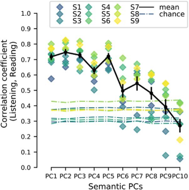
Similarity between listening and reading semantic PC projections. The correlation coefficient between listening and reading semantic PC projections are shown for the first 10 semantic PCs and each individual participant separately. Each colored diamond shape indicate one participant and the mean correlation coefficient across participants is indicated by the black solid line. Error bars indicate SEM across the correlation coefficients for all participants. The colored dotted lines at the bottom indicate chance level correlation for each semantic PC and participant as computed by a permutation test. At least the first five semantic PC projections are significantly correlated between listening and reading. This shows that the individual dimensions of the semantic maps in Figure 4 where the first three semantic PCs are displayed are similar across the two modalities.

Is semantic tuning consistent across modalities at the single-voxel level?

Here, we sought to determine whether all the dimensions of semantic representation depend on input modality at the level of single voxels. To do this, the 985 semantic model weights estimated for each voxel during listening were correlated with those semantic model weights estimated during reading.

Figure 6a shows the correlation coefficient between estimated listening and reading model weights for each voxel, mapped onto the cortical surface of one individual participant. Listening and reading model weights are strongly correlated in many regions within the semantic system including bilateral temporal, parietal, and prefrontal cortices (red voxels in Fig. 6a). These voxels are also significantly well predicted by the semantic model in both modalities. Voxels whose model weights are not correlated are located in few scattered voxels in the bilateral sensory cortex, intraparietal sulcus, and in PFC (white voxels). This suggests that voxels that are semantically selective in listening and reading modalities (red) represent similar semantic information. Figure 6b summarizes the relation between within-modality voxelwise model prediction accuracy and semantic tuning, for each voxel. Each voxel is a single point in the scatterplot, and the correlation between the estimated listening and reading model weights is indicated by the color saturation. Semantic tuning is more similar for voxels that are semantically selective in both modalities (red) than for those that are well predicted in one modality only (blue or green). Negatively correlated voxels are mostly in sensory regions and are not well predicted by the semantic model in either modality. In general, individual voxels located within the semantic system are selective to similar semantic features during both listening and reading.

Figure 6.

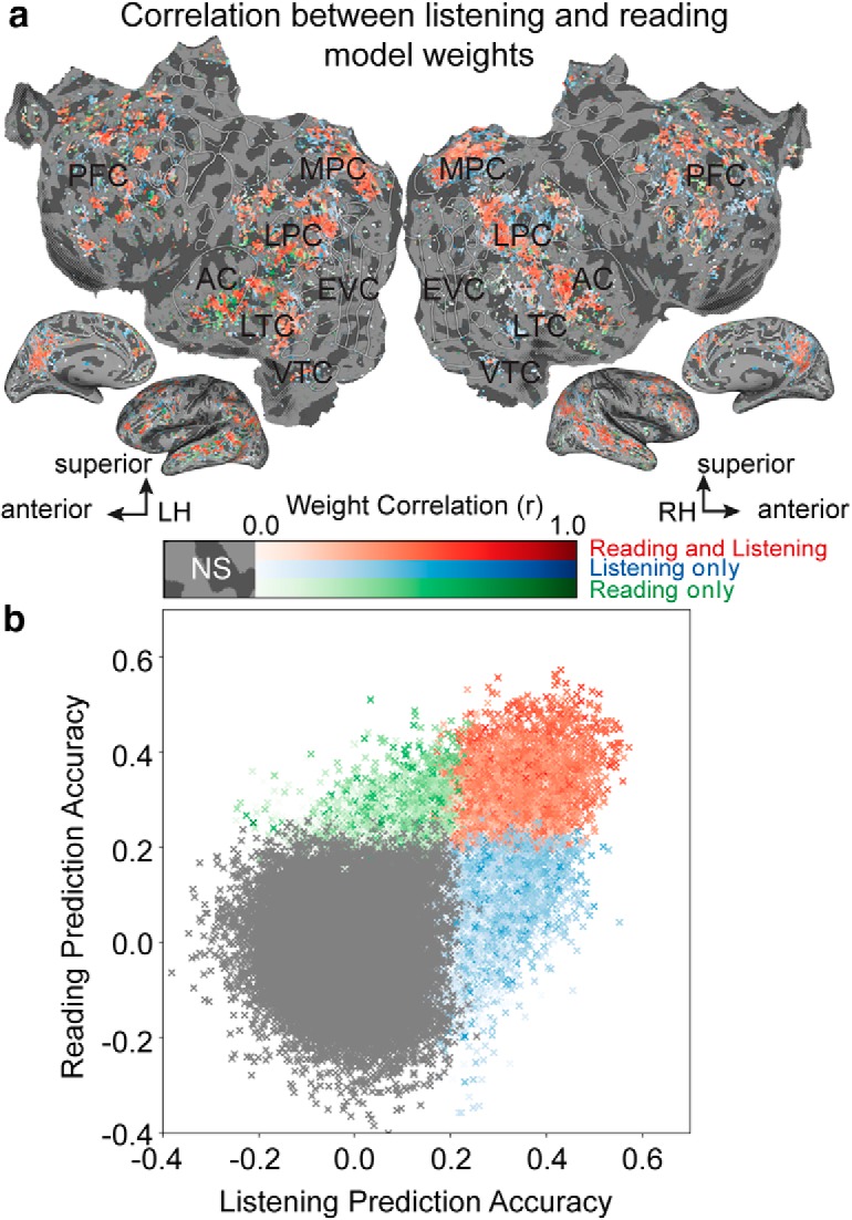
Voxelwise similarity of semantic tuning across listening and reading. Semantic model weights estimated during listening and reading were correlated for each voxel separately. a, Correlation coefficient between listening and reading model weights are shown on the flattened cortical surface of one participant. Red voxels are those that are semantically selective in both modalities. Blue voxels are those that are semantically selective in listening, but not reading. Green voxels are those that are semantically selective in reading, but not listening. Gray voxels are not semantically selective in either modality. Color saturation describes the strength of voxel weight correlations. The stronger the color the higher is the correlation between listening and reading model weights. Voxels in the semantic system have similar semantic tuning across all the semantic features. LH, Left hemisphere; RH, right hemisphere; NS, not significant; EVC, early visual cortex. This suggests that across the 985 semantic features semantic information is represented similarly in both modalities in the semantic system. b, Relationship between within-modality model prediction accuracy and semantic tuning. Listening (x-axis) versus reading (y-axis) prediction accuracy is shown in a scatterplot where each point corresponds to a single voxel in a. The correlation between the listening and reading model weights is indicated by color saturation and is the same as in a. Semantic tuning is more similar for voxels that are semantically selective in both modalities (red) than for those that are selective in one modality only (blue and green). Gray voxels are not semantically selective in either modality. This suggests that voxels that are well predicted in both modalities represent similar semantic information.

Can a voxelwise model fit to one modality predict responses to the other modality?

If the semantic representation in most of the semantic system is modality-invariant then voxel models fit to one modality should accurately predict responses in the other modality. Figures 7 and 8 show cross-modal predictions for all voxels in all participants. Figure 7 shows prediction accuracy for a model fit to voxel responses evoked during listening, but predicting responses evoked during reading. Figure 8 shows prediction accuracy for a model fit to responses evoked during reading, but predicting responses evoked during listening. In both figures voxels whose predictions were not statistically significant are shown in gray (p > 0.05, FDR corrected). In both cases, voxels in bilateral temporal, parietal, and prefrontal cortices are well predicted across modalities. Voxels that are not well predicted cross-modally are located in sensory cortices.

Figure 7.

Semantically amodal voxels as shown by cross-modal predictions (Listening predicting Reading) in all participants. Estimated semantic model weights in the listening modality were used to predict BOLD activity to the held-out validation story in the reading modality. a, Accuracy of voxelwise models estimated during listening predicting reading responses, shown on the same participant's flattened cortical surface as in Figure 2. Prediction accuracy is given by the color scale. Voxels that are well predicted appear yellow or white, voxel predictions that are not statistically significant are shown in gray (p > 0.05, FDR corrected). (LH, left hemisphere; RH, right hemisphere; NS, not significant; Si, Subject i; EVC, early visual cortex). b, Accuracy of voxelwise models estimated during listening predicting reading responses, shown for all other participants. The format is the same as in a. The semantic model estimated in listening accurately predicts voxel responses in reading within the semantic system including bilateral temporal (LTC, VTC), parietal (LPC, MPC), and prefrontal cortices (PFC).

Figure 8.

Semantically amodal voxels as shown by cross-modal predictions (Reading predicting Listening) in all participants. Estimated semantic model weights in the reading modality were used to predict BOLD activity to the held-out validation story in the listening modality. a, Accuracy of voxelwise models estimated during reading predicting listening responses, shown on the same participant's flattened cortical surface as in Figure 2. Prediction accuracy is given by the color scale. Voxels that are well predicted appear yellow or white, voxel predictions that are not statistically significant are shown in gray (p > 0.05, FDR corrected). (LH, left hemisphere; RH, right hemisphere; NS, not significant; Si, Subject i; EVC, early visual cortex). b, Accuracy of voxelwise models estimated during reading predicting listening responses, shown for all other participants. The format is the same as in a. The semantic model estimated in reading accurately predicts voxel responses in listening within the semantic system including bilateral temporal (LTC, VTC), parietal (LPC, MPC), and prefrontal cortices (PFC).

Figure 9 shows a summary map of the relationship between cross-modality predictions and within-modality predictions, for each voxel and all participants. Summary statistics for the two cross-modality predictions were computed by taking the average cross-modality prediction accuracy (per voxel average of Figs. 7 and 8). Summary statistics for the two within-modality predictions were computed by taking the maximum within-modality prediction accuracy (per voxel maximum of Fig. 2a,b). The mean cross-modality prediction accuracy and the maximum within-modality prediction accuracy per voxel were then mapped onto the same participant's flattened cortical surface. Inspection of Figure 9 allows us to identify voxels that are well predicted both within and across modality. Most voxels that are well predicted within and across modality are located in the semantic system (white voxels in Fig. 9). Outside the semantic system, some voxels on the border to visual cortex and voxels surrounding the temporal parietal junction are well predicted within modality but not across modality (orange voxels in Fig. 9). (Note, however, that within-modality data were collected largely within sessions, and between-modality data were collected across sessions. Thus, within-modality prediction accuracy is likely to be somewhat higher than between-modality accuracy for this reason alone.) This result demonstrates that the distribution of semantically selective voxels in most of the semantic system is independent of the modality.

Figure 9.

Semantically amodal voxels for all participants. Comparison of voxels that are well predicted across modalities versus within modalities. a, The average cross-modality prediction accuracy and the maximum of the within-modality prediction accuracy per voxel are both plotted on the flattened cortical surface of the same participant's flattened cortical surface as in Figure 2. (L2R: Listening predicting Reading, R2L: Reading predicting Listening; L2L: Listening predicting Listening, R2R: Reading predicting Reading; Si: Subject i; LH, left hemisphere; RH, right hemisphere; NS, not significant).Orange voxels are well predicted only within-modality. White voxels are well predicted both within and across modality (in most of the semantic system). Blue voxels are well predicted only across modality. Voxels that are not significant in within- or cross-modality predictions are shown in gray. b, Same comparison plotted for all other participants. The format is the same as in a. Voxels within the semantic system represent semantic information independent of modality.

Discussion

The experiments presented here were designed to determine whether semantic information obtained during listening and reading are represented within a common underlying semantic system. In separate fMRI sessions participants listened to a spoken story and read a stream of words visually (RSVP using time-locked transcripts of spoken stories). We used VM to estimate semantic selectivity across the entire cerebral cortex, in individual participants, in each voxel separately and in two different presentation modalities (listening and reading).

Our experiments provide three lines of evidence in support of the hypothesis that semantic representations throughout most of the semantic system are invariant to presentation modality. First, voxels in most of the semantic system (temporal, parietal, and prefrontal cortices) are well predicted by the semantic model in each modality independently (Figs. 2, 3). Second, the estimated model weights and the semantic maps are similar between listening and reading (Figs. 4, 5, 6). Third, voxelwise models estimated from one modality (e.g., listening) accurately predict responses in the other modality (e.g., reading) throughout most of the semantic system (Figs. 7, 8, 9).

Our results demonstrate in a single study that semantically amodal voxels span most of the bilateral semantic system. It has been previously proposed that subsequent to early sensory processing, the pathways for processing information by listening or reading converge in semantically selective regions (Chee et al., 1999; Carpentier et al., 2001; Booth et al., 2002; Cohen et al., 2004; Constable et al., 2004; Spitsyna et al., 2006; Jobard et al., 2007; Patterson et al., 2007; Buchweitz et al., 2009; Liuzzi et al., 2017). Different studies have emphasized different brain regions such as the left anterior temporal lobe, left ventral angular gyrus, left inferotemporal cortex, a region left lateral to the visual word form area (VWFA), left MTG, and the left IFG. Bilateral activations have been reported previously in epileptic patients (Carpentier et al., 2001) or when complex stimuli such as narrative has been used (Spitsyna et al., 2006; Jobard et al., 2007; Regev et al., 2013). Our study shows that semantically amodal voxels are bilaterally distributed across many regions of the temporal, parietal and prefrontal cortices (Figs. 3, 4, 5, 6). Specifically, we show amodal semantic representation in bilateral precuneus, temporal parietal junction (TPJ), angular gyrus (AG), anterior to posterior STS, sPMv, Broca's area and inferior frontal gyrus (IFG).

One previous report noted that listening and reading evoke different levels of brain activity in anterior and posterior left DLPFC (Regev et al., 2013). However, Regev et al. (2013) did not model linguistic features directly. Therefore, it is unclear whether the differences they identified within left DLPFC are due to differences in semantic representation or some other aspect of linguistic information (e.g., syntax). In our study, we focused solely on semantic representations and our results suggest that semantic representations do not differ between listening and reading in left DLPFC. However, it is possible that this structure may represent other types of linguistic information differently during listening and reading.

One striking difference between our results and those reported in earlier studies is that we find a large network of semantically selective regions that are independent of the presentation modality, whereas previous studies reported a few amodal semantic regions located mostly in the left hemisphere (Petersen et al., 1989; Chee et al., 1999; Jobard et al., 2007; Buchweitz et al., 2009; Liuzzi et al., 2017). There are three possible factors that contribute to this discrepancy. First, we used rich narrative language as stimuli to study cross-modal semantic representation (Fig. 1). Previous studies have shown that complex linguistic stimuli such as narrative stories activate many more brain regions than single words or short sentences (Mazoyer et al., 1993; Xu et al., 2005; Jobard et al., 2007; Lerner et al., 2011). Hence, differences in signal-to-noise ratio can account for fewer number of amodal regions identified in previous cross-modality studies that use single words or short sentences.

Second, our VM approach used explicit semantic features, which allowed us to identify brain regions that consistently respond to specific semantic information across different modalities (Figs. 1, 2, 3, 4, 5, 6). To our knowledge, only one previous study of cross-modal representation has used explicit semantic features to model brain activity patterns related to semantics (Liuzzi et al., 2017). That study used as stimuli twenty-four single words derived from only six animate categories, and showed cross-modal representations within left pars triangularis. However, the most likely reason that the Liuzzi et al. (2017) study only identified one region as semantically amodal is that single word presentations elicit little brain activity.

Third, the present study is the first that reveals the amodal representation of semantic information during listening and reading in single participants (Fig. 1). In contrast, most previous neuroimaging studies of language perform comparisons at the group level after transforming individual participant data into a standardized brain space (e.g., MNI or Talairach space). However, the anatomical normalization procedures used in these studies tend to smooth and mask the substantial individual variability in language processing (Caramazza, 1986; Steinmetz and Seitz, 1991; Fedorenko and Kanwisher, 2009). Therefore, studies performing intersubject averaging might average away meaningful signal and fail to find significant relationships (Fedorenko and Kanwisher, 2009). Indeed, projecting our results into a standard brain space and averaging across individuals reduces prediction performance within modality across much of the brain (cf. Figs. 3a, 2). This result demonstrates that it is important to study cross-modal language representations in individual participants.

Our naturalistic experiment and VM provides a powerful and efficient method for identifying amodal representations in individual human brains. However, the semantic feature space that we used here is only one possible way of representing semantics (Mitchell et al., 2008; Huth et al., 2016; Pereira et al., 2018), and it has some limitations. For example, when people listen to or read a story they likely employ conceptual knowledge at long time scales beyond those using for computing semantic features (Yeshurun et al., 2017). Furthermore, semantic comprehension involves metaphors, humor, sarcasm and narrative information that is not reflected in the current semantic model. It is possible that these unmodeled properties of natural language might have different, modality-specific representations in the brain.

In sum, we demonstrate modality-independent semantic selectivity in most of the bilateral semantic system. The semantic maps recovered in this study show that semantic tuning in individual participants is very similar across the two modalities. Our findings are consistent with the view that sensory regions process unimodal information related to low-level processing of spoken or written language, whereas high-level regions process modality invariant semantic information. Furthermore, our results reveal that modality invariant semantic representations are not isolated in a few left-lateralized regions, but are instead present in many bilaterally distributed regions of the semantic system.

References

- Adelson EH, Bergen JR (1985) Spatiotemporal energy models for the perception of motion. J Opt Soc Am A 2:284–299. 10.1364/JOSAA.2.000284 [DOI] [PubMed] [Google Scholar]
- Amunts K, Lenzen M, Friederici AD, Schleicher A, Morosan P, Palomero-Gallagher N, Zilles K (2010) Broca's Region: Novel Organizational Principles and Multiple Receptor Mapping. PLoS Biol. 8:e1000489. 10.1371/journal.pbio.1000489 [DOI] [PMC free article] [PubMed] [Google Scholar]
- Andor D, Alberti C, Weiss D, Severyn A, Presta A, Ganchev K, Petrov S, Collins M (2016) Globally normalized transition-based neural networks. arXiv:1603.06042. Available at https://arxiv.org/abs/1603.06042.
- Benjamini Y, Hochberg Y (1995) Controlling the false discovery rate: a practical and powerful approach to multiple testing. J R Stat Soc Ser B 57:289–300. [Google Scholar]
- Bergstra JS, Bardenet R, Bengio Y, Kégl B (2011) Algorithms for hyper-parameter optimization. In Advances in Neural Information Processing Systems 24, pp 2546–2554. New York: Curran Associates, Inc. [Google Scholar]
- Binder JR, Desai RH, Graves WW, Conant LL (2009) Where is the semantic system? A critical review and meta-analysis of 120 functional neuroimaging studies. Cereb Cortex 19:2767–2796. 10.1093/cercor/bhp055 [DOI] [PMC free article] [PubMed] [Google Scholar]
- Boersma P, Weenink DJM (2001) Praat, a system for doing phonetics by computer. Glot International 5:341–345. [Google Scholar]
- Booth JR, Burman DD, Meyer JR, Gitelman DR, Parrish TB, Mesulam MM (2002) Modality independence of word comprehension. Hum Brain Mapp 16:251–261. 10.1002/hbm.10054 [DOI] [PMC free article] [PubMed] [Google Scholar]
- Buchweitz A, Mason RA, Tomitch LM, Just MA (2009) Brain activation for reading and listening comprehension: an fMRI study of modality effects and individual differences in language comprehension. Psychol Neurosci 2:111–123. 10.3922/j.psns.2009.2.003 [DOI] [PMC free article] [PubMed] [Google Scholar]
- Caramazza A. (1986) On drawing inferences about the structure of normal cognitive systems from the analysis of patterns of impaired performance: the case for single-patient studies. Brain Cogn 5:41–66. 10.1016/0278-2626(86)90061-8 [DOI] [PubMed] [Google Scholar]
- Carpentier A, Pugh KR, Westerveld M, Studholme C, Skrinjar O, Thompson JL, Spencer DD, Constable RT (2001) Functional MRI of language processing: dependence on input modality and temporal lobe epilepsy. Epilepsia 42:1241–1254. 10.1046/j.1528-1157.2001.35500.x [DOI] [PubMed] [Google Scholar]
- Chee MW, O'Craven KM, Bergida R, Rosen BR, Savoy RL (1999) Auditory and visual word processing studied with fMRI. Hum Brain Mapp 7:15–28. 10.1002/(SICI)1097-0193(1999)7:1<15::AID-HBM2>3.0.CO;2-6 [DOI] [PMC free article] [PubMed] [Google Scholar]
- Church KW, Hanks P (1990) Word association norms, mutual information, and lexicography. Comput Linguist 16:22–29. [Google Scholar]
- Cohen L, Jobert A, Le Bihan D, Dehaene S (2004) Distinct unimodal and multimodal regions for word processing in the left temporal cortex. Neuroimage 23:1256–1270. 10.1016/j.neuroimage.2004.07.052 [DOI] [PubMed] [Google Scholar]
- Corbetta M, Akbudak E, Conturo TE, Snyder AZ, Ollinger JM, Drury HA, Linenweber MR, Petersen SE, Raichle ME, Van Essen DC, Shulman GL (1998) A common network of functional areas for attention and eye movements. Neuron 21:761–773. 10.1016/S0896-6273(00)80593-0 [DOI] [PubMed] [Google Scholar]
- Constable RT, Pugh KR, Berroya E, Mencl WE, Westerveld M, Ni W, Shankweiler D (2004) Sentence complexity and input modality effects in sentence comprehension: an fMRI study. Neuroimage 22:11–21. 10.1016/j.neuroimage.2004.01.001 [DOI] [PubMed] [Google Scholar]
- Çukur T, Nishimoto S, Huth AG, Gallant JL (2013) Attention during natural vision warps semantic representation across the human brain. Nat Neurosci 16:763–770. 10.1038/nn.3381 [DOI] [PMC free article] [PubMed] [Google Scholar]
- Dale AM, Fischl B, Sereno MI (1999) Cortical surface-based analysis: I. segmentation and surface reconstruction. Neuroimage 9:179–194. 10.1006/nimg.1998.0395 [DOI] [PubMed] [Google Scholar]
- Deerwester S, Dumais ST, Furnas GW, Landauer TK, Harshman R (1990) Indexing by latent semantic analysis. J Am Soc Inf Sci 41:391–407. 10.1002/(SICI)1097-4571(199009)41:6<391::AID-ASI1>3.0.CO;2-9 [DOI] [Google Scholar]
- de Heer WA, Huth AG, Griffiths TL, Gallant JL, Theunissen FE (2017) The hierarchical cortical organization of human speech processing. J Neurosci 37:6539–6557. 10.1523/JNEUROSCI.3267-16.2017 [DOI] [PMC free article] [PubMed] [Google Scholar]
- Démonet JF, Chollet F, Ramsay S, Cardebat D, Nespoulous JL, Wise R, Rascol A, Frackowiak R (1992) The anatomy of phonological and semantic processing in normal subjects. Brain 115:1753–1768. 10.1093/brain/115.6.1753 [DOI] [PubMed] [Google Scholar]
- Démonet JF, Price C, Wise R, Frackowiak RS (1994) Differential activation of right and left posterior sylvian regions by semantic and phonological tasks: a positron-emission tomography study in normal human subjects. Neurosci Lett 182:25–28. 10.1016/0304-3940(94)90196-1 [DOI] [PubMed] [Google Scholar]
- Devlin JT, Jamison HL, Matthews PM, Gonnerman LM (2004) Morphology and the internal structure of words. Proc Natl Acad Sci U S A 101:14984–14988. 10.1073/pnas.0403766101 [DOI] [PMC free article] [PubMed] [Google Scholar]
- Diakidoy IAN, Stylianou P, Karefillidou C, Papageorgiou P (2005) The relationship between listening and reading comprehension of different types of text at increasing grade levels. Read Psychol 26:55–80. 10.1080/02702710590910584 [DOI] [Google Scholar]
- Downing PE, Jiang Y, Shuman M, Kanwisher N (2001) A cortical area selective for visual processing of the human body. Science 293:2470–2473. 10.1126/science.1063414 [DOI] [PubMed] [Google Scholar]
- Epstein R, Kanwisher N (1998) A cortical representation of the local visual environment. Nature 392:598–601. 10.1038/33402 [DOI] [PubMed] [Google Scholar]
- Fedorenko E, Kanwisher N (2009) Neuroimaging of language: why Hasn't a clearer picture emerged? Linguistics Compass 3:839–865. [Google Scholar]
- Forster KI. (1970) Visual perception of rapidly presented word sequences of varying complexity. Percept Psychophys 8:215–221. 10.3758/BF03210208 [DOI] [Google Scholar]
- Gao JS, Huth AG, Lescroart MD, Gallant JL (2015) Pycortex: an interactive surface visualizer for fMRI. Front Neuroinform 9:23. 10.3389/fninf.2015.00023 [DOI] [PMC free article] [PubMed] [Google Scholar]
- Grosbras MH, Lobel E, Van de Moortele PF, LeBihan D, Berthoz A (1999) An anatomical landmark for the supplementary eye fields in human revealed with functional magnetic resonance imaging. Cereb Cortex 9:705–711. 10.1093/cercor/9.7.705 [DOI] [PubMed] [Google Scholar]
- Halgren E, Dale AM, Sereno MI, Tootell RB, Marinkovic K, Rosen BR (1999) Location of human face-selective cortex with respect to retinotopic areas. Hum Brain Mapp 7:29–37. 10.1002/(SICI)1097-0193(1999)7:1<29::AID-HBM3>3.0.CO;2-R [DOI] [PMC free article] [PubMed] [Google Scholar]
- Hansen KA, Kay KN, Gallant JL (2007) Topographic organization in and near human visual area V4. J Neurosci 27:11896–11911. 10.1523/JNEUROSCI.2991-07.2007 [DOI] [PMC free article] [PubMed] [Google Scholar]
- Huth AG, Nishimoto S, Vu AT, Gallant JL (2012) A continuous semantic space describes the representation of thousands of object and action categories across the human brain. Neuron 76:1210–1224. 10.1016/j.neuron.2012.10.014 [DOI] [PMC free article] [PubMed] [Google Scholar]
- Huth AG, de Heer WA, Griffiths TL, Theunissen FE, Gallant JL (2016) Natural speech reveals the semantic maps that tile human cerebral cortex. Nature 532:453–458. 10.1038/nature17637 [DOI] [PMC free article] [PubMed] [Google Scholar]
- Jenkinson M, Smith S (2001) A global optimisation method for robust affine registration of brain images. Med Image Anal 5:143–156. 10.1016/S1361-8415(01)00036-6 [DOI] [PubMed] [Google Scholar]
- Jenkinson M, Bannister P, Brady M, Smith S (2002) Improved optimization for the robust and accurate linear registration and motion correction of brain images. Neuroimage 17:825–841. 10.1006/nimg.2002.1132 [DOI] [PubMed] [Google Scholar]
- Jobard G, Vigneau M, Mazoyer B, Tzourio-Mazoyer N (2007) Impact of modality and linguistic complexity during reading and listening tasks. Neuroimage 34:784–800. 10.1016/j.neuroimage.2006.06.067 [DOI] [PubMed] [Google Scholar]
- Kanwisher N, McDermott J, Chun MM (1997) The fusiform face area: a module in human extrastriate cortex specialized for face perception. J Neurosci 17:4302–4311. 10.1523/JNEUROSCI.17-11-04302.1997 [DOI] [PMC free article] [PubMed] [Google Scholar]
- Kluyver T, Ragan-Kelley B, Pérez F, Granger B, Bussonnier M, Frederic J, Kelley K, Hamrick J, Grout J, Corlay S, Ivanov P, Avila D, Abdalla S, Willing C, Team Jupyter Development (2016) Jupyter Notebooks—a publishing format for reproducible computational workflows. In ELPUB, pp 87–90. Amsterdam:IOS Press. [Google Scholar]
- Lerner Y, Honey CJ, Silbert LJ, Hasson U (2011) Topographic Mapping of a Hierarchy of Temporal Receptive Windows Using a Narrated Story. J Neurosci 31:2906–2915. 10.3389/fncom.2015.00135 [DOI] [PMC free article] [PubMed] [Google Scholar]
- Lescroart MD, Stansbury DE, Gallant JL (2015) Fourier power, subjective distance, and object categories all provide plausible models of BOLD responses in scene-selective visual areas. Front Comput Neurosci 9:135. 10.3389/fncom.2015.00135 [DOI] [PMC free article] [PubMed] [Google Scholar]
- Liuzzi AG, Bruffaerts R, Peeters R, Adamczuk K, Keuleers E, De Deyne S, Storms G, Dupont P, Vandenberghe R (2017) Cross-modal representation of spoken and written word meaning in left pars triangularis. Neuroimage 150:292–307. 10.1016/j.neuroimage.2017.02.032 [DOI] [PubMed] [Google Scholar]
- Lund K, Burgess C (1996) Producing high-dimensional semantic spaces from lexical co-occurrence. Behavior Research Methods, Instruments, & Computers 28:203–208. 10.3758/BF03204766 [DOI] [Google Scholar]
- Mazoyer BM, Tzourio N, Frak V, Syrota A, Murayama N, Levrier O, Salamon G, Dehaene S, Cohen L, Mehler J (1993) The cortical representation of speech. J Cogn Neurosci 5:467–479. 10.1162/jocn.1993.5.4.467 [DOI] [PubMed] [Google Scholar]
- McLaren K. (1976) XIII-the development of the CIE 1976 (L* a* b*) uniform colour space and colour-difference formula. J Soc Dye Colour 92:338–341. [Google Scholar]
- Michael EB, Keller TA, Carpenter PA, Just MA (2001) fMRI investigation of sentence comprehension by eye and by ear: modality fingerprints on cognitive processes. Hum Brain Mapp 13:239–252. 10.1002/hbm.1036 [DOI] [PMC free article] [PubMed] [Google Scholar]
- Mitchell TM, Shinkareva SV, Carlson A, Chang KM, Malave VL, Mason RA, Just MA (2008) Predicting human brain activity associated with the meanings of nouns. Science 320:1191–1195. 10.1126/science.1152876 [DOI] [PubMed] [Google Scholar]
- Nakamura K, Kawashima R, Sato N, Nakamura A, Sugiura M, Kato T, Hatano K, Ito K, Fukuda H, Schormann T, Zilles K (2000) Functional delineation of the human occipito-temporal areas related to face and scene processing: a PET study. Brain 123:1903–1912. 10.1093/brain/123.9.1903 [DOI] [PubMed] [Google Scholar]
- Nakamura K, Dehaene S, Jobert A, Le Bihan D, Kouider S (2005) Subliminal Convergence of Kanji and Kana words: further evidence for functional parcellation of the posterior temporal cortex in visual word perception. J Cogn Neurosci 17:954–968. 10.1162/0898929054021166 [DOI] [PubMed] [Google Scholar]
- Naselaris T, Kay KN, Nishimoto S, Gallant JL (2011) Encoding and decoding in fMRI. Neuroimage 56:400–410. 10.1016/j.neuroimage.2010.07.073 [DOI] [PMC free article] [PubMed] [Google Scholar]
- Nishimoto S, Vu AT, Naselaris T, Benjamini Y, Yu B, Gallant JL (2011) Reconstructing visual experiences from brain activity evoked by natural movies. Curr Biol 21:1641–1646. 10.1016/j.cub.2011.08.031 [DOI] [PMC free article] [PubMed] [Google Scholar]
- Nunez-Elizalde AO, Huth AG, Gallant JL (2019) Voxelwise encoding models with non-spherical multivariate normal priors. Neuroimage 197:482–492. 10.1016/j.neuroimage.2019.04.012 [DOI] [PubMed] [Google Scholar]
- Oldfield RC. (1971) The assessment and analysis of handedness: the Edinburgh inventory. Neuropsychologia 9:97–113. 10.1016/0028-3932(71)90067-4 [DOI] [PubMed] [Google Scholar]
- Oliphant TE. (2006) A guide to NumPy, Vol 1, p 85 USA: Trelgol Publishing. [Google Scholar]
- Oliphant TE. (2007) SciPy: open source scientific tools for python. Comput Sci Eng 9:10–20. [Google Scholar]
- Patterson K, Nestor PJ, Rogers TT (2007) Where do you know what you know? The representation of semantic knowledge in the human brain. Nat Rev Neurosci 8: 976–987. 10.1038/nrn2277 [DOI] [PubMed] [Google Scholar]
- Paus T. (1996) Location and function of the human frontal eye-field: a selective review. Neuropsychologia 34:475–483. 10.1016/0028-3932(95)00134-4 [DOI] [PubMed] [Google Scholar]
- Penfield W, Boldrey E (1937) Somatic motor and sensory representation in the cereb cortex of man as studied by electrical stimulation. Brain 60:389–443. 10.1093/brain/60.4.389 [DOI] [Google Scholar]
- Penny WD, Friston K, Ashburner J, Kiebel S, Nichols T (2007) Statistical parametric mapping: the analysis of functional brain images. Amsterdam: Elsevier. [Google Scholar]
- Pereira F, Lou B, Pritchett B, Ritter S, Gershman SJ, Kanwisher N, Botvinick M, Fedorenko E (2018) Toward a universal decoder of linguistic meaning from brain activation. Nat Commun 9:963. 10.1038/s41467-018-03068-4 [DOI] [PMC free article] [PubMed] [Google Scholar]
- Pérez F, Granger BE (2007) IPython: a system for interactive scientific computing. Computing in Science & Engineering 9:21–29. 10.1109/mcse.2007.53 [DOI] [Google Scholar]
- Petersen SE, Fox PT, Posner MI, Mintun M, Raichle ME (1989) Positron emission tomographic studies of the processing of singe words. J Cogn Neurosci 1:153–170. 10.1162/jocn.1989.1.2.153 [DOI] [PubMed] [Google Scholar]
- Price CJ. (2010) The anatomy of language: a review of 100 fMRI studies published in 2009. Ann N Y Acad Sci 1191:62–88. 10.1111/j.1749-6632.2010.05444.x [DOI] [PubMed] [Google Scholar]
- Price CJ. (2012) A review and synthesis of the first 20years of PET and fMRI studies of heard speech, spoken language and reading. Neuroimage 62:816–847. 10.1016/j.neuroimage.2012.04.062 [DOI] [PMC free article] [PubMed] [Google Scholar]
- Regev M, Honey CJ, Simony E, Hasson U (2013) Selective and invariant neural responses to spoken and written narratives. J Neurosci 33:15978–15988. 10.1523/JNEUROSCI.1580-13.2013 [DOI] [PMC free article] [PubMed] [Google Scholar]
- Rissman J, Eliassen JC, Blumstein SE (2003) An event-related fMRI investigation of implicit semantic priming. J Cogn Neurosci 15:1160–1175. 10.1162/089892903322598120 [DOI] [PubMed] [Google Scholar]
- Rubin DL, Hafer T, Arata K (2000) Reading and listening to oral-based versus literate-based discourse. Commun Educ 49:121–133. 10.1080/03634520009379200 [DOI] [Google Scholar]
- Scott SK, Blank CC, Rosen S, Wise RJ (2000) Identification of a pathway for intelligible speech in the left temporal lobe. Brain 123:2400–2406. 10.1093/brain/123.12.2400 [DOI] [PMC free article] [PubMed] [Google Scholar]
- Spiridon M, Fischl B, Kanwisher N (2006) Location and spatial profile of category-specific regions in human extrastriate cortex. Hum Brain Mapp 27:77–89. 10.1002/hbm.20169 [DOI] [PMC free article] [PubMed] [Google Scholar]
- Spitsyna G, Warren JE, Scott SK, Turkheimer FE, Wise RJ (2006) Converging language streams in the human temporal lobe. J Neurosci 26:7328–7336. 10.1523/JNEUROSCI.0559-06.2006 [DOI] [PMC free article] [PubMed] [Google Scholar]
- Stansbury DE, Naselaris T, Gallant JL (2013) Natural scene statistics account for the representation of scene categories in human visual cortex. Neuron 79:1025–1034. 10.1016/j.neuron.2013.06.034 [DOI] [PMC free article] [PubMed] [Google Scholar]
- Steinmetz H, Seitz RJ (1991) Functional anatomy of language processing: neuroimaging and the problem of individual variability. Neuropsychologia 29:1149–1161. 10.1016/0028-3932(91)90030-C [DOI] [PubMed] [Google Scholar]
- Tikhonov AN, Arsenin VY (1977) Solutions of ill-posed problems. New York: Winston. [Google Scholar]
- Tootell RB, Reppas JB, Kwong KK, Malach R, Born RT, Brady TJ, Rosen BR, Belliveau JW (1995) Functional analysis of human MT and related visual cortical areas using magnetic resonance imaging. J Neurosci 15:3215–3230. 10.1523/JNEUROSCI.15-04-03215.1995 [DOI] [PMC free article] [PubMed] [Google Scholar]
- Turney P, Pantel P (2010) From frequency to meaning: vector space models of semantics. J Artif Intell Res 37:141–188. 10.1613/jair.2934 [DOI] [Google Scholar]
- Vandenberghe R, Price C, Wise R, Josephs O, Frackowiak RS (1996) Functional anatomy of a common semantic system for words and pictures. Nature 383:254–256. 10.1038/383254a0 [DOI] [PubMed] [Google Scholar]
- Vigneau M, Beaucousin V, Hervé PY, Duffau H, Crivello F, Houdé O, Mazoyer B, Tzourio-Mazoyer N (2006) Meta-analyzing left hemisphere language areas: phonology, semantics, and sentence processing. Neuroimage 30:1414–1432. 10.1016/j.neuroimage.2005.11.002 [DOI] [PubMed] [Google Scholar]
- Watson AB, Ahumada AJ Jr (1985) Model of human visual-motion sensing. J Opt Soc Am A 2:322–341. [DOI] [PubMed] [Google Scholar]
- Wehbe L, Murphy B, Talukdar P, Fyshe A, Ramdas A, Mitchell T (2014) Simultaneously uncovering the patterns of brain regions involved in different story reading subprocesses. PLoS One 9:e112575. 10.1371/journal.pone.0112575 [DOI] [PMC free article] [PubMed] [Google Scholar]
- Xu J, Kemeny S, Park G, Frattali C, Braun A (2005) Language in context: emergent features of word, sentence, and narrative comprehension. Neuroimage 25:1002–1015. 10.1016/j.neuroimage.2004.12.013 [DOI] [PubMed] [Google Scholar]
- Yeshurun Y, Swanson S, Simony E, Chen J, Lazaridi C, Honey CJ, Hasson U (2017) Same story, different story. Psychol Sci 28:307–319. 10.1177/0956797616682029 [DOI] [PMC free article] [PubMed] [Google Scholar]
- Yuan J, Liberman M (2008) Speaker identification on the SCOTUS corpus. Journal of the Acoustical Society of America 123: 3878. [Google Scholar]
- Zilles K, Amunts K (2018) Cytoarchitectonic and receptorarchitectonic organization in Broca's region and surrounding cortex. Curr Opin Behav Sci 21:93–105. 10.1016/j.cobeha.2018.02.011 [DOI] [Google Scholar]