Abstract
Diffusion MRI (DMRI) is a powerful tool for studying early brain development and disorders. However, the typically low spatio-angular resolution of DMRI diminishes structural details and limits quantitative analysis to simple diffusion models. This problem is aggravated for infant DMRI since (i) the infant brain is significantly smaller than that of an adult, demanding higher spatial resolution to capture subtle structures; and (ii) the typically limited scan time of unsedated infants poses significant challenges to DMRI acquisition with high spatio-angular resolution. Post-acquisition super-resolution (SR) is an important alternative for increasing the resolution of DMRI data without prolonging acquisition times. However, most existing methods focus on the SR of only either the spatial domain (x-space) or the diffusion wavevector domain (q-space). For more effective resolution enhancement, we propose a framework for joint SR in both spatial and wavevector domains. More specifically, we first establish the signal relationships in x-q space using a robust neighborhood matching technique. We then harness the signal relationships to regularize the ill-posed inverse problem associated with the recovery of high-resolution data from their low-resolution counterpart. Extensive experiments on synthetic, adult, and infant DMRI data demonstrate that our method is able to recover high-resolution DMRI data with remarkably improved quality.
Keywords: Diffusion MRI, Super Resolution, Neighborhood Matching, Regularization
1. Introduction
Diffusion MRI (DMRI) has been widely employed to investigate white matter changes associated with early brain development and disorders (Cascio et al., 2007; Dubois et al., 2014; Alexander et al., 2007). For instance, it has been shown using diffusion tensor imaging that mean diffusivity (MD) decreases and fractional anisotropy (FA) increases during brain development (Cascio et al., 2007; Dubois et al., 2014). Moreover, MD increase and FA decrease are found in the corpus callosum in patients with autism spectrum disorder (Alexander et al., 2007).
Despite its great utility, the typically low spatio-angular resolution of DMRI diminishes structural details and limits quantitative analysis to simple diffusion models. In practice, there is a trade-off between resolution, signal-to-noise-ratio (SNR), and acquisition time. Increasing spatial resolution often comes at the cost of SNR when the acquisition time is limited. Increasing angular resolution typically requires prolonged acquisition time, since it is directly related to the number of diffusion-weighted (DW) images that are acquired in association with the diffusion-sensitizing gradient directions. Acquiring high-resolution data for infants is even more challenging. First, the infant brain is significantly smaller than that of an adult (Knick-meyer et al., 2008; Li et al., 2012), demanding higher spatial resolution to capture subtle structures. Second, the acquisition time of infant DMRI data is significantly limited. For instance, in the Human Connectome Project (HCP) (Van Essen et al., 2012), the DMRI scan time is about an hour per adult. However, in the Baby Connectome Project (BCP) (Fallik, 2016; Howell et al., 2019), the acquisition time is limited to less than 15 minutes, since scanning of infants is typically performed when they are asleep and has to be terminated if they wake up. The possibility of infants awakening is heightened by loud acoustic noise and sudden vibrations resulting from the rapid switching of gradient amplitude and polarity typical in DMRI (McJury PhD and Frank, 2000).
An alternative to acquisition-based methods is post-acquisition super-resolution (SR) (Nedjati-Gilani et al., 2008; Calamante et al., 2010; Manjón et al., 2010; Alexander et al., 2017; Chen et al., 2017; Tuch, 2004; Descoteaux et al., 2007; Tanno et al., 2017). Existing SR methods can be divided into two categories based on their outcomes: derived diffusion quantities (Nedjati-Gilani et al., 2008; Calamante et al., 2010; Alexander et al., 2017) or DW images (Manjón et al., 2010; Chen et al., 2017; Tuch, 2004; Descoteaux et al., 2007; Tanno et al., 2017). Nedjati-Gilani et al. (2008) introduced a method for estimating orientations and volume fractions of fiber populations on a sub-voxel scale. Calamante et al. (2010) gained sub-voxel insights into white matter by computing local tract density using a very high number of fiber tracts given by whole-brain tractography. Alexander et al. (2017) proposed a technique, called image quality transfer, that learns low-resolution (LR) to high-resolution (HR) mappings of patches for different microstructural index maps. These methods are however restricted to specific derived quantities, e.g., fiber orientations, track density map, or microstructure index maps. On the other hand, SR of DW images affords greater flexibility in subsequent analysis (Manjón et al., 2010; Alexander et al., 2017; Chen et al., 2017; Tuch, 2004; Descoteaux et al., 2007; Tanno et al., 2017). For x-space SR, Manjón et al. (2010) propose a patch-based SR framework to improve the resolution of MR images by iteratively performing non-local means (NLM) reconstruction and correcting for intensity mean consistency. Tanno et al. (2017) proposed a technique called Bayesian image quality transfer for SR of DW images using mean apparent propagator data with convolutional neural networks. For q-space SR, the most common approaches are interpolation using spherical radial basis functions (SRBFs) (Tuch, 2004) or spherical harmonics (SHs) (Descoteaux et al., 2007). A common limitation of these methods is that SR is performed separately for spatial and wavevector domains, neglecting the relation between them.
In this paper, we propose an x-q space SR (XQ-SR) framework that harnesses self-similar information in the joint x-q space of DMRI. More specifically, we first establish the relationships of signals in x-q space using a robust neighborhood matching technique (Chen et al., 2019). We then use the established relationships to regularize the ill-posed inverse problem associated with the recovery of high resolution (HR) DMRI data, both spatially and angularly, from its LR counterpart. To the best of our knowledge, XQ-SR is the first method for spatio-angular SR that uses self-similarity information in the joint x-q space. To verify its effectiveness, we performed experiments on various datasets, including synthetic, adult, and infant data. Extensive experimental results demonstrate that XQ-SR outperforms various state-of-the-art methods and is capable of improving remarkably the quality of HR DMRI data.
The rest of the paper is organized as follows. In Section 2, we provide a detailed description of XQ-SR. In Section 3, we demonstrate the effectiveness of XQ-SR with synthetic data, adult DMRI data, and infant DMRI data. In Section 4, we provide further discussion on this work. In Section 5, we conclude our work.
2. Method
XQ-SR aims to jointly increase the spatio-angular resolution. This is achieved by harnessing the non-local self-similar information in the joint x-q space. Self-similar information is identified with the help of the robust x-q space neighborhood matching technique described in (Chen et al., 2019), which caters to even highly curved white matter structures where traditional x-space neighborhood matching methods are typically less effective.
2.1. Establishing Signal Relationships in Joint x-q Space
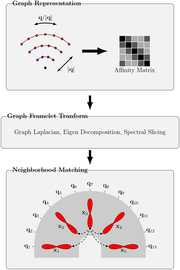
We establish the relationships of signals in joint x-q space using a robust neighborhood matching technique described in (Chen et al., 2019). As illustrated in Fig. 1, this procedure involves three steps. The first two steps employ (i) Graph representation and (ii) Graph framelet transform (GFT) to extract neighborhood features for each sampling point in x-q space. The features are used in the third step, (iii) Neighborhood matching, for establishing signal correspondences.
Figure 1: Overview.
(Graph Representation) Representing the q-space sampling domain using a graph with affinity matrix determined by kernels for diffusion gradient directions and strengths. (Graph Framelet Transform) Feature computation by spectral decomposition. (Neighborhood Matching) Correspondence matching in x-q space. Note that q-space is generally 3D; 2D illustration is used here for simplicity.
Specifically, we first represent the q-space sampling domain using a graph with an affinity matrix with elements determined by the products of two kernels — one for the diffusion gradient directions {q/|q|} and the other for gradient strengths {|q|}. The signals corresponding to different gradient directions and strengths at each voxel location can be viewed as a function defined on the graph. We perform GFT (Yap et al., 2016a) on this function to compute the neighborhood features for the nodes of the graph. The key idea of GFT is to slice the frequency spectrum of the graph in a multi-scale fashion by using a set of masks. The spectrum is obtained by performing Eigen decomposition on the graph Laplacian. A detailed description of GFT can be found in (Yap et al., 2016a; Dong, 2017). Given a point in x-q space associated with an x-space index i and a q-space index k, the first two steps will generate a feature vector f(i, k) for the point. Finally, in the third step, we compute the similarity weight between points (i, k) and (j, l) in the x-q space using a Gaussian function of the distance between the feature vectors, i.e.,
| (1) |
Note that this allows correspondences to be established between points in the x-q space even in highly curved white matter structures, as illustrated in Fig. 1. For more details on x-q space neighborhood matching, please refer to (Chen et al., 2019).
2.2. Resolution Enhancement Using x-q Space Regularization
Let dLR be the signal vector containing the diffusion-attenuated signals of all points in x-space and q-space in the LR DMRI data. Our aim is to recover its HR counterpart dHR by solving an inverse problem regularized by the signal relationships in x-q space. We define our objective function as
| (2) |
where Dx and Dq are respectively binary matrices representing downsampling operators in x-space and q-space, with a 1 in each row indicating an element in dHR that will be retained. Bx represents an x-space smoothing operator realized via convolution with a Gaussian kernel. λ is a regularization term controlling the trade-off between the data fidelity term and the regularization term r(dHR). The regularization term r(dHR) takes into account the signal relationships determined using neighborhood matching and is defined as
| (3) |
where Ω is the image domain and is the x-q space search neighborhood for point (i, k) and Ei,k is a matrix representing the operator that extracts the diffusion signal at point (i, k). The regularization term encourages non-local smoothness (Protter et al., 2009) by requiring each diffusion signal to be represented by its matching signals.
2.3. Optimization
2.3.1. Algebraic Simplification
To minimize the objective function, we set the derivative of (2) to zero:
| (4) |
where O = DqDxBx representing the operations associated with HR to LR. Matrix O resembles the blurring matrix described in Section 2.2, but is row-downsampled. The number of rows is determined by the number of x-q space sampling points in the LR DMRI data. Based on the definition of r(dHR), we have
| (5) |
Observe that (i) the neighborhood is symmetric (i.e., if , then ), and (ii) the weights are symmetric (i.e., w(i, k; j, l) = w(j, l; i, k)) (Protter et al., 2009). Therefore, we have
| (6) |
and
| (7) |
Simplifying (5) using (6) and (7) gives
| (8) |
where
| (9) |
| (10) |
Therefore, (4) becomes
| (11) |
Finally, we have
| (12) |
Algorithm 1.
Conjugate Gradient Method
| Require: Matrix M, vector v and initialization . | |
| 1: | Let , p0 = r0 and k = 0 |
| 2: | loop |
| 3: | |
| 4: | |
| 5: | rk+1 = rk – αkMpk |
| 6: | if then |
| 7: | end loop |
| 8: | end if |
| 9: | |
| 10: | pk+1 = rk+1 + βkpk |
| 11: | k = k +1 |
| 12: | end loop |
| 13: | return |
2.3.2. Conjugate Gradient (CG) Method
Equation (12) is a large-scale system of linear equations, which can be solved directly but involves the inversion of a very large matrix (Protter et al., 2009). For greater efficiency, we utilize the CG method (Shewchuk, 1994) to solve the problem. A detailed proof of the applicability of CG to our problem is provided in the appendix. The algorithm is summarized in Algorithm 1.
2.3.3. Initialization
Prior to SR, we first perform signal transformation as described in (Koay et al., 2009) so that noise becomes Gaussian distributed. We then perform spatial upsampling using an NLM-based method introduced in (Manjón et al., 2010) and angular upsampling using spherical harmonics (Descoteaux et al., 2007). The upsampled data is used as initialization, , in our algorithm. Based on , we perform x-q space neighborhood matching, as described in Section 2.1, to obtain the similarity weights.
3. Experiments
3.1. Datasets
3.1.1. Synthetic Data
For quantitative evaluation, we generated a noise-free HR dataset using phantomαs (Caruyer et al., 2014) and the fiber geometric setting of ISBI 2013 HARDI challenge1. The gradients used in data simulation were consistent with the adult data described in the next section, i.e., b = 1000, 2000, 3000 s/mm2, 90 gradient directions per shell.
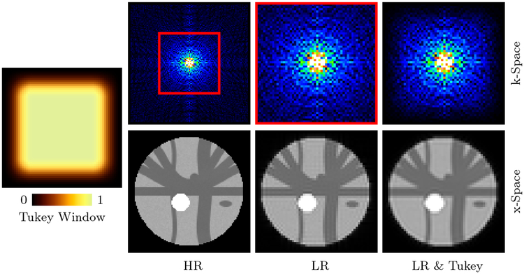
We downsampled the simulated HR dataset to generate its LR counterpart. Downsampling in x-space involves the following steps (see Fig. 2): (i) Fourier transform of the HR DW images. (ii) Removal of high-frequency content based on downsampling ratio (2 in our case). (iii) Filtering using Tukey window (Fong, 2005) to reduce Gibbs ringing. (iv) Inverse Fourier transform to obtain the LR DW images. Downsampling in q-space was then carried out by uniformly sampling half of the gradient directions in each shell. Finally, we added noise of different levels (SNR = 10, 20, 30, measured with respect to S0 = 1000) to the LR data.
Figure 2: Downsampling in x-Space.
LR image generated by (i) Extracting the low-frequency component (red rectangle) of the frequency spectrum of the HR image, and (ii) Filtering with a Tukey window.
3.1.2. Adult Data
The DMRI dataset of one subject randomly selected from the Human Connectome Project (HCP) (Van Essen et al., 2013) was used for evaluation. The dataset was acquired using a customized Siemens 3T Connectome Skyra MR scanner with the following imaging protocol: 145 × 174 imaging matrix, 1.25 × 1.25 × 1.25 mm3 resolution, TE=89 ms, TR=5,500 ms, 32-channel receiver coil (Van Essen et al., 2013). Signal transformation as described in (Koay et al., 2009) was performed so that noise becomes Gaussian distributed. The images were downsampled to generate the corresponding LR counterpart as done with the synthetic dataset.
3.1.3. Infant Data
Three infant subjects from the Baby Connectome Project (Howell et al., 2019) were scanned postnatally at 2, 27, and 48 weeks. All data were acquired using a Siemens 3T Magnetom Prisma MR scanner with the following protocol: 140 × 105 imaging matrix, 1.5 × 1.5 × 1.5 mm3 resolution, TE=88 ms, TR=2,365 ms, 32-channel receiver coil, b = 500, 1000, 1500, 2000, 2500, 3000 s/mm2, and a total of 144 non-collinear gradient directions. All enrolled subjects had written informed consent provided by parents/guardians. The experimental protocols were approved by the Institutional Review Board of the University of North Carolina (UNC) School of Medicine. Signal transformation as in (Koay et al., 2009) was performed.
3.2. Parameter Settings
In all experiments, we set the parameters for neighborhood matching in according to the parameter settings suggested in (Chen et al., 2019). Specifically, we set β = 0.1, s = 1, and θ = 30°, where β is a parameter controlling the bandwidth of the Gaussian function in Eq. (1), s is the x-space search radius, and θ is the q-space search angle. For the parameters used in SR, we performed grid search and found that λ = 100 and tol = 0.1 gave the best results.
3.3. Baseline Methods
Existing SR methods focus on one aspect of SR, i.e., either enhancing the spatial resolution or the angular resolution. Therefore, we used four hybrid SR methods for comparison. SR in x-space was performed using either linear interpolation or NLM-based upsampling (Manjón et al., 2010). SR in q-space upsampling was performed using either SRBFs (Tuch, 2004) or SHs (Descoteaux et al., 2007). For brevity, the four combinations are denoted as Linear+SRBF, Linear+SH, NLM+SRBF, and NLM+SH.
3.4. Evaluation Methods
Qualitative and quantitative experiments were performed:
- Peak signal-to-noise ratio (PSNR): PSNR is used for quantitative evaluation, and is defined as
where RMSE is the root-mean-square-error between an image and the ground truth, MAX is the maximum signal value. A higher PSNR value implies that the image is closer to the ground truth.(13) FA images: We compute FA images using the iterative weighted tensor fitting method presented in (Salvador et al., 2005).
Absolute difference (AD) and mean normalized absolute difference (MNAD): The AD of FA with respect to the ground truth was evaluated. MNAD is computed by dividing AD with the ground truth.
Root mean squared error (RMSE): We computed the voxel-wise RMSE of a set of DW images, viewed as a single vector-valued image, with respect to the ground truth.
Fiber ODFs: We computed fiber orientation distribution functions (ODFs) using the method presented in (Yap et al., 2016b) for visual inspection.
3.5. Results
3.5.1. Synthetic Data
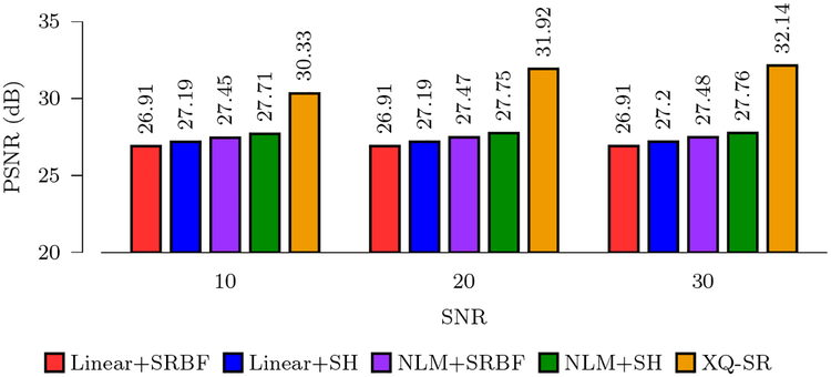
Figure 3 shows the PSNR values computed using reconstructed HR DMRI data and the ground truth. It can be observed that XQ-SR gives the highest PSNR values for all noise levels. A higher PSNR value indicates better resemblance with the ground truth. Compared with the second-best method, NLM+SH, XQ-SR yields an improvement of 4.19 dB at SNR = 30.
Figure 3: PSNR Comparison.
Quantitative evaluation using synthetic data.
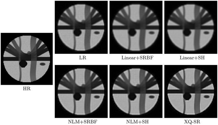
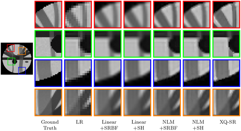
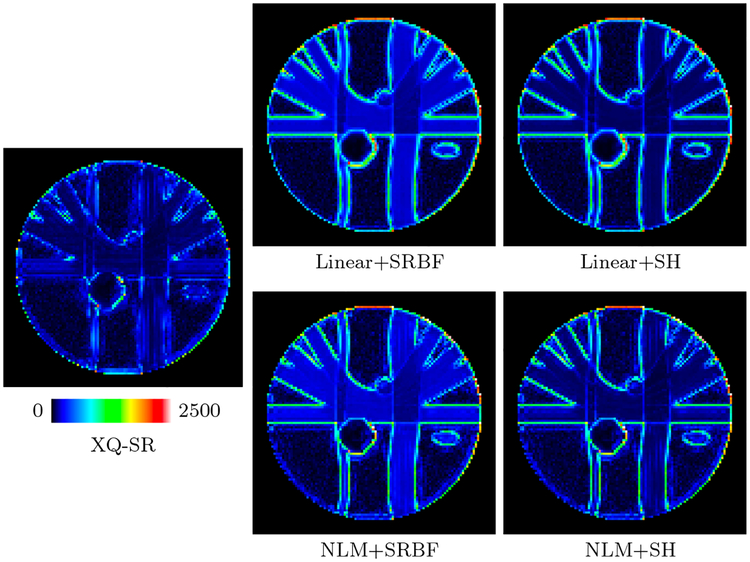
The DW images, shown in Fig. 4, further demonstrate the advantages of XQ-SR. Compared with other methods, XQ-SR is capable of recovering HR DW images with more structural details, especially at boundaries, as illustrated in the close-up views in Fig. 5. Moreover, Fig. 6 shows that XQ-SR dramatically reduces RMSE, indicating that its outcome is closer to ground truth.
Figure 4: DW Images – Synthetic Data.
Comparison of DW images for b = 1,000 s/mm2 and SNR = 30.
Figure 5: Close-Up Views of DW Images – Synthetic Data.
Local comparison of DW images for b = 1,000 s/mm2 and SNR = 30.
Figure 6: RMSE Maps – Synthetic Data.
Comparison of RMSE maps for the synthetic data.
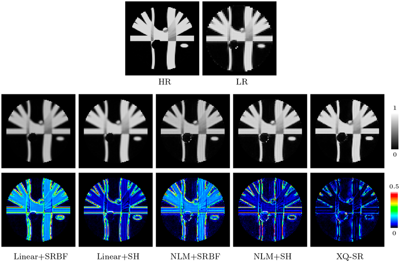
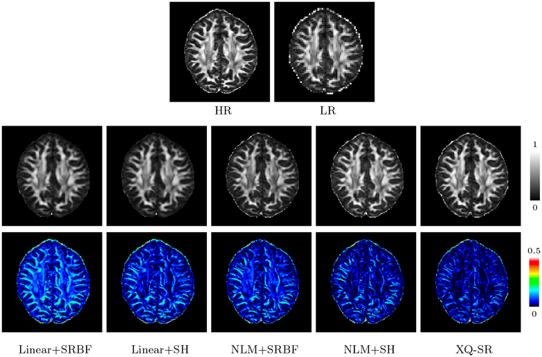
We further computed the FA images to evaluate the effects of SR on diffusion indices. Figure 7, indicates that XQ-SR gives an FA image with sharp structural boundaries. The advantages of XQ-SR is further confirmed with the AD maps (bottom row of Fig. 7), where XQ-SR yields results closest to the ground truth with the lowest AD values.
Figure 7: FA Images – Synthetic Data.
AD comparison of FA images. Mean AD values are shown at the top left corners. The background was excluded when computing the mean values.
3.5.2. Adult Data
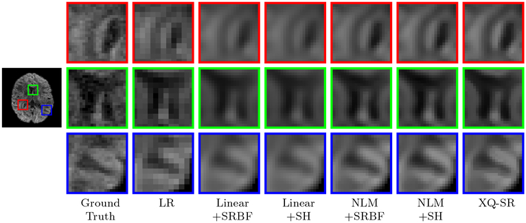
The observations from Fig. 5 are confirmed by Fig. 8 with real data, where XQ-SR again shows greater preservation of structural details, especially in the cortical regions, as shown by the close-up views.
Figure 8: Close-Up Views of DW Images – Adult Data.
Local comparison of DW images for b = 1,000 s/mm2.
Figure 9 indicates that XQ-SR gives an FA image with sharper structural details and is closer to the ground truth. The AD maps, shown in the bottom row of Fig. 9, indicate that XQ-SR gives an AD map with much lower values. These observations are consistent with Fig. 7.
Figure 9: FA Images and AD Maps – HCP Data.
AD comparison of FA images. Mean AD values are shown at the top left corners. The background was excluded when computing the mean values.
3.5.3. Infant Data
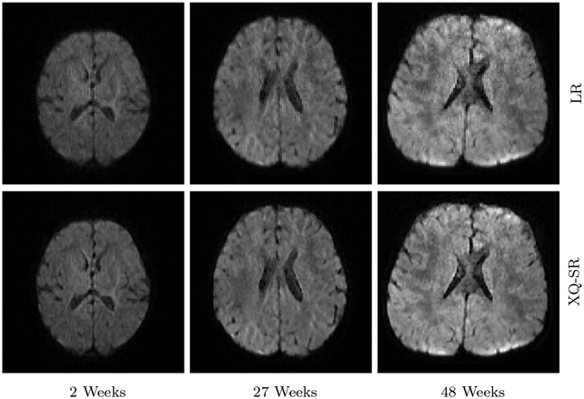
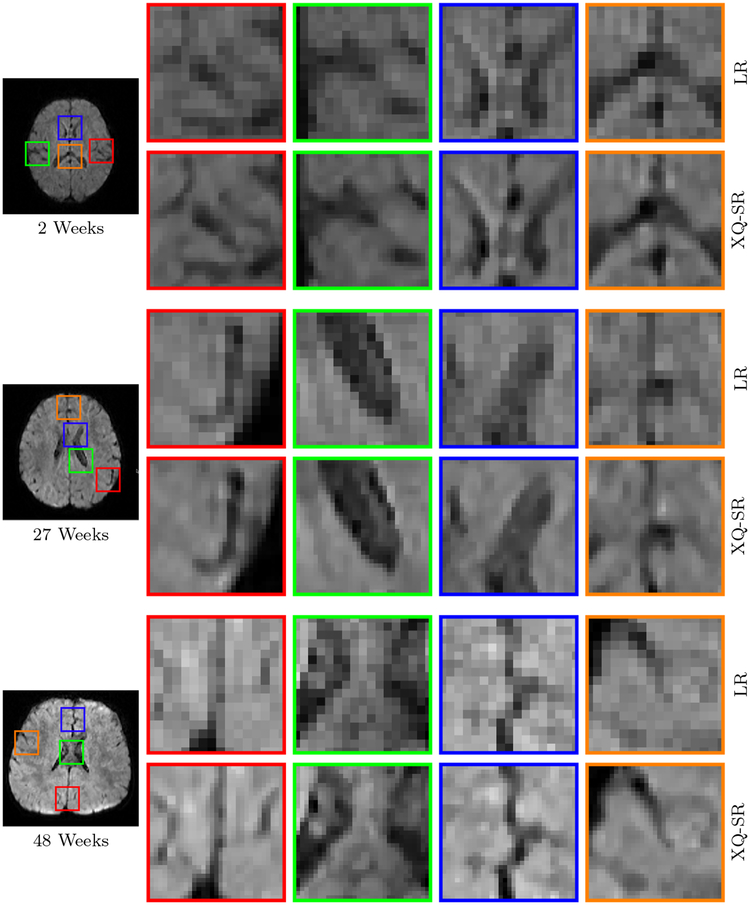
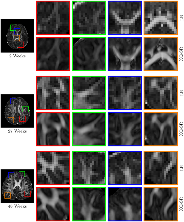
We further utilized XQ-SR to improve the resolution of infant DMRI data. The DW images, shown in Fig. 10 and 11, indicate that, for all time points, XQ-SR improves the sharpness and clarity of structural details.
Figure 10: DWI Images – Infant Data.
Comparison of DW images for b = 1,000 s/mm2.
Figure 11: Close-Up Views of DW Images – Infant Data.
Regional close-up views of DW images, shown in Fig. 10.
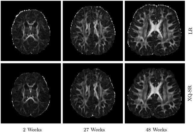
Figures 12 and 13 further demonstrate that XQ-SR yields FA images with richer structural details compared with the LR images.
Figure 12: FA Images – Infant Data.
Comparison of FA images of infant DMRI data.
Figure 13: Close-Up Views of FA Images – Infant Data.
Regional close-up views of FA images, shown in Fig. 12.
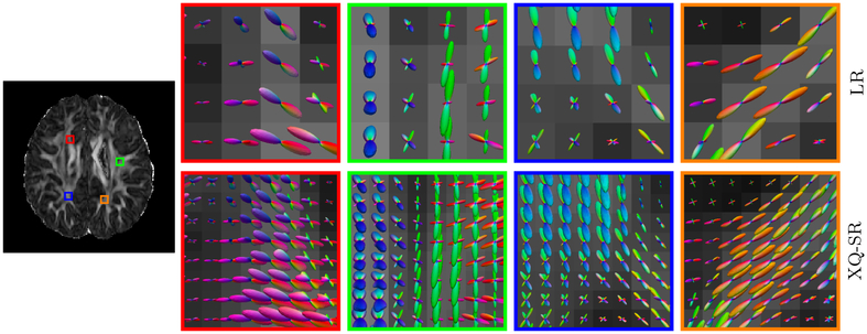
Figure 14 indicates that XQ-SR (i) gives clean and coherent fiber ODFs, (ii) well preserves the fiber orientation information in the LR DMRI data, and (iii) provides improved fiber orientation information, especially in regions with complex fiber geometries, such as crossings.
Figure 14: Fiber ODFs – Infant Data.
Comparison of fiber ODFs of infant DMRI data.
4. Discussion
High-resolution DMRI data reconstructed using XQ-SR retain more structural details and better preserves the values of diffusion indices. As illustrated in Figs. 7 and 9, the baseline methods result in large FA errors. This is mainly caused by the smoothing effect of these methods, which reduces the sharpness of the diffusion signal profile. In contrast, XQ-SR utilizes x-q space signal relationships for regularization and preserves well the sharpness of diffusion signal profiles, and thus retaining FA values that are closer to the ground truth.
XQ-SR depends on the accurate estimation of the relationships between the diffusion-attenuated signals. In practice, we can re-estimate the neighborhood matching weights from the reconstructed HR DMRI data, and then utilize the updated weights for iterative SR reconstruction. However, our experimental results indicate that the contribution of this strategy is minimal, and iterative SR significantly extends the computational time. Therefore, we did not perform weight re-estimation in our experiments.
XQ-SR is built upon our work reported in (Chen et al., 2017). However, compared with (Chen et al., 2017), XQ-SR (i) focuses on spatio-angular resolution enhancement, rather than angular enhancement only, and (ii) employes the conjugate gradient method instead of fixed point iteration.
Using an 8-core Xeon CPU, XQ-SR takes about 6.28 hours to process one infant dataset (see Section 3.5.3). Currently, XQ-SR was implemented using C++ based on the Insight Segmentation and Registration Toolkit (ITK)2. Speed can be potentially improved by further parallelization or GPU implementation.
Recently, some advanced MRI reconstruction approaches were proposed to recover high spatio-angular resolution DMRI data. For instance, Mani et al. (2015) utilize compressed sensing (CS) to recover HR DMRI data from under-sampled k-q space data. The associated ill-posed inverse problem is regularized by imposing sparsity on the coefficients of ODFs and by reducing the TV of the HR DMRI data. A method called 6D-CS-DMRI (Cheng et al., 2015) was developed to cater to multi-shell DMRI. This method harnesses the sparsity of the coefficients of the ensemble average propagator (EAP) in the estimation of HR DMRI and EAP data from the data sub-sampled in both 3D k-space and 3D q-space. More recently, Ning et al. (2016) proposed a method to reconstruct a very HR DMRI dataset from multiple LR DMRI datasets. This method regularizes both x-space and q-space based on spatial smoothness, which is imposed by TV, and the sparsity of ODF coefficients. Despite the promising performance of these methods, they require specially designed imaging protocols, limiting their widespread application. In contrast, XQ-SR can be applied to existing DMRI data acquired using conventional imaging protocols.
Learning-based methods have been shown to be effective for super-resolution (Alexander et al., 2017; Tanno et al., 2017), fiber orientation estimation (Koppers and Merhof, 2016; Ye and Prince, 2017), and microstructure estimation (Golkov et al., 2016; Ye, 2017; Ye et al., 2019, 2018). Deep leaning techniques improve estimation tissue microstructural properties from DMRI data that are highly undersampled in q-space (Golkov et al., 2016; Ye, 2017; Ye et al., 2019, 2018). Graph convolutional neural networks (GCNNs) yield promising performance in longitudinal prediction of infant DMRI data (Kim et al., 2018; Hong et al., 2019c) and acceleration of DMRI data acquisition (Hong et al., 2019a,b). In the future, we will explore utilizing GCNNs to jointly increase the resolution of DMRI data in both x-space and q-space.
Currently, we only employ x-q space signal relationships for the regularization. In the future, we can improve XQ-SR by integrating other advanced regularization terms into our framework, such as the total generalized variation (TGV) (Bredies et al., 2010), low rank (Shi et al., 2016; Zhou et al., 2018, 2019), and bilateral total variation (Farsiu et al., 2004). In particular, TGV is known as a generalization of the total variation, considering both the first and second derivative of a function, thus is able to avoid the stair-casing effect caused by TV regularization (Bredies et al., 2010). This extension is expected to improve the quality of the reconstructed HR DMRI data.
The neighborhood matching technique used in XQ-SR is a general framework for establishing the signal relationships in x-q space. This technique can be further utilized to improve a number of algorithms, including atlas building (Saghafi et al., 2017; Kim et al., 2017; Yang et al., 2017), ODF estimation (Chen et al., 2016; Ye et al., 2016), voxel-based morphometry (Chen et al., 2015), etc.
5. Conclusion
In this work, we have proposed a regularization framework for the spatio-angular resolution enhancement of DMRI data. In this framework, the signal relationships in x-q space are employed to regularize the ill-posed inverse problem associated with recovering HR DMRI data from its LR counterpart. Experiments using synthetic and adult DMRI data demonstrate that our method outperforms various state-of-the-art methods, both qualitatively and quantitatively. We have also demonstrated the utility of our method in improving the quality of infant DMRI data.
Highlights.
XQ-SR enhances the resolution of DMRI data in both spatial and wavevector domains.
XQ-SR utilizes signal relationships in joint x-q space to regularize the ill-posed inverse problem associated with resolution enhancement.
Extensive experimental results demonstrate that XQ-SR is able to recover high-resolution DMRI data with remarkably improved quality.
Acknowledgment
This work was supported in part by NIH grants (NS093842, EB022880, EB006733, and 1U01MH110274) and the e orts of the UNC/UMN Baby Connectome Project Consortium. Data were provided in part by the Human Connectome Project, WU-Minn Consortium (Principal Investigators: David Van Essen and Kamil Ugurbil; 1U54MH091657) funded by the 16 NIH Institutes and Centers that support the NIH Blueprint for Neuroscience Research; and by the McDonnell Center for Systems Neuroscience at Washington University.
Appendix
CG requires that M be symmetric and positive-definite.
Symmetry: Matrix M is the sum of three terms, i.e., O⊤O, Z and W. The first matrix, O⊤O, is symmetric since (O⊤O)⊤ = O⊤O. The second matrix, Z, is a diagonal matrix with each diagonal element , and is therefore symmetric. Since the search regions and weights are both symmetric, W is symmetric as well. Matrix M is therefore symmetric.
- Positive-definiteness: We can separate M into two parts, i.e., O⊤O and Z–W. First, O⊤O is positive-semidefinite, since for an arbitrarily non-zero vector z⊤, we have
Second, matrix W can be viewed as a graph adjacency matrix relating points in the x-q space, with Z being the corresponding degree matrix. The Laplacian matrix L = Z–W is positive-semidefinite and t⊤Lt = 0 when t = t0 = c(1, 1, ⋯,1)⊤. However, since in our case O is a nonnegative downsampling and blurring operator, we have , and hence M is positive-definite.(14)
Footnotes
Publisher's Disclaimer: This is a PDF file of an unedited manuscript that has been accepted for publication. As a service to our customers we are providing this early version of the manuscript. The manuscript will undergo copyediting, typesetting, and review of the resulting proof before it is published in its final citable form. Please note that during the production process errors may be discovered which could affect the content, and all legal disclaimers that apply to the journal pertain.
References
- Alexander AL, Lee JE, Lazar M, Boudos R, DuBray MB, Oakes TR, Miller JN, Lu J, Jeong EK, McMahon WM, et al. , 2007. Diffusion tensor imaging of the corpus callosum in Autism. NeuroImage 34, 61–73. [DOI] [PubMed] [Google Scholar]
- Alexander DC, Zikic D, Ghosh A, Tanno R, Wottschel V, Zhang J, Kaden E, Dyrby TB, Sotiropoulos SN, Zhang H, et al. , 2017. Image quality transfer and applications in diffusion MRI. NeuroImage 152, 283–298. [DOI] [PubMed] [Google Scholar]
- Bredies K, Kunisch K, Pock T, 2010. Total generalized variation. SIAM Journal on Imaging Sciences 3, 492–526. [Google Scholar]
- Calamante F, Tournier JD, Jackson GD, Connelly A, 2010. Track-density imaging (TDI): super-resolution white matter imaging using whole-brain track-density mapping. NeuroImage 53, 1233–1243. [DOI] [PubMed] [Google Scholar]
- Caruyer E, Daducci A, Descoteaux M, Houde JC, Thiran JP, Verma R, 2014. Phantomas: a flexible software library to simulate diffusion MR phantoms, in: ISMRM. [Google Scholar]
- Cascio CJ, Gerig G, Piven J, 2007. Diffusion tensor imaging: application to the study of the developing brain. Journal of the American Academy of Child and Adolescent Psychiatry 46, 213–223. [DOI] [PubMed] [Google Scholar]
- Chen G, Dong B, Zhang Y, Lin W, Shen D, Yap PT, 2019. Denoising of infant diffusion MRI data via graph framelet matching in x-q space. IEEE Transactions on Medical Imaging. [DOI] [PMC free article] [PubMed] [Google Scholar]
- Chen G, Dong B, Zhang Y, Shen D, Yap PT, 2017. q-space upsampling using x-q space regularization, in: Medical Image Computing and Computer-Assisted Intervention (MICCAI), Springer; pp. 620–628. [DOI] [PMC free article] [PubMed] [Google Scholar]
- Chen G, Zhang P, Li K, Wee CY, Wu Y, Shen D, Yap PT, 2015. Block-based statistics for robust non-parametric morphometry, in: International Workshop on Patch-based Techniques in Medical Imaging, Springer International Publishing; pp. 62–70. [DOI] [PMC free article] [PubMed] [Google Scholar]
- Chen G, Zhang P, Li K, Wee CY, Wu Y, Shen D, Yap PT, 2016. Improving estimation of fiber orientations in diffusion MRI using inter-subject information sharing. Scientific Reports 6, 37847. [DOI] [PMC free article] [PubMed] [Google Scholar]
- Cheng J, Shen D, Basser PJ, Yap PT, 2015. Joint 6d k-q space compressed sensing for accelerated high angular resolution diffusion MRI, in: International Conference on Information Processing in Medical Imaging, Springer; pp. 782–793. [DOI] [PMC free article] [PubMed] [Google Scholar]
- Descoteaux M, Angelino E, Fitzgibbons S, Deriche R, 2007. Regularized, fast, and robust analytical Q-ball imaging. Magnetic resonance in medicine 58, 497–510. [DOI] [PubMed] [Google Scholar]
- Dong B, 2017. Sparse representation on graphs by tight wavelet frames and applications. Applied and Computational Harmonic Analysis 42, 452–479. [Google Scholar]
- Dubois J, Dehaene-Lambertz G, Kulikova S, Poupon C, Hüppi PS, Hertz-Pannier L, 2014. The early development of brain white matter: a review of imaging studies in fetuses, newborns and infants. Neuroscience 276, 48–71. [DOI] [PubMed] [Google Scholar]
- Fallik D, 2016. The human connectome project turns to mapping brain development, from birth through early childhood. Neurology Today 16, 7–8. [Google Scholar]
- Farsiu S, Robinson MD, Elad M, Milanfar P, 2004. Fast and robust multiframe super resolution. IEEE Transactions on Image Processing 13, 1327–1344. [DOI] [PubMed] [Google Scholar]
- Fong W, 2005. Handbook of MRI pulse sequences. Medical Physics 32, 1452–1452. [Google Scholar]
- Golkov V, Dosovitskiy A, Sperl JI, Menzel MI, Czisch M, Sämann P, Brox T, Cremers D, 2016. q-space deep learning: twelve-fold shorter and model-free diffusion MRI scans. IEEE Transactions on Medical Imaging 35, 1344–1351. [DOI] [PubMed] [Google Scholar]
- Hong Y, Chen G, Yap PT, Shen D, 2019a. Multifold acceleration of diffusion MRI via deep learning reconstruction from slice-undersampled data, in: International Conference on Information Processing in Medical Imaging, Springer; pp. 530–541. [DOI] [PMC free article] [PubMed] [Google Scholar]
- Hong Y, Chen G, Yap PT, Shen D, 2019b. Reconstructing high-quality diffusion MRI data from orthogonal slice-undersampled data using graph convolutional neural networks, in: Medical Image Computing and Computer-Assisted Intervention (MICCAI). [DOI] [PMC free article] [PubMed] [Google Scholar]
- Hong Y, Kim J, Chen G, Lin W, Yap PT, Shen D, 2019c. Longitudinal prediction of infant diffusion MRI data via graph convolutional adversarial networks. IEEE Transactions on Medical Imaging. [DOI] [PMC free article] [PubMed] [Google Scholar]
- Howell BR, Styner MA, Gao W, Yap PT, Wang L, Baluyot K, Yacoub E, Chen G, Potts T, Salzwedel A, Li G, Gilmore JH, Piven J, Smith JK, Shen D, Ugurbil K, Zhu H, Lin W, Elison JT, 2019. The UNC/UMN Baby Connectome Project (BCP): An overview of the study design and protocol development. NeuroImage 185, 891–905. [DOI] [PMC free article] [PubMed] [Google Scholar]
- Kim J, Chen G, Lin W, Yap PT, Shen D, 2017. Graph-constrained sparse construction of longitudinal diffusion-weighted infant atlases, in: Medical Image Computing and Computer-Assisted Intervention (MIC-CAI), Springer; pp. 49–56. [DOI] [PMC free article] [PubMed] [Google Scholar]
- Kim J, Hong Y, Chen G, Lin W, Yap PT, Shen D, 2018. Graph-based deep learning for prediction of longitudinal infant diffusion MRI data, in: MICCAI Workshop on Computational Diffusion MRI. Springer, pp. 133–141. [DOI] [PMC free article] [PubMed] [Google Scholar]
- Knickmeyer RC, Gouttard S, Kang C, Evans D, Wilber K, Smith JK, Hamer RM, Lin W, Gerig G, Gilmore JH, 2008. A structural MRI study of human brain development from birth to 2 years. Journal of Neuroscience 28, 12176–12182. [DOI] [PMC free article] [PubMed] [Google Scholar]
- Koay CG, Özarslan E, Basser PJ, 2009. A signal transformational framework for breaking the noise floor and its applications in MRI. Journal of Magnetic Resonance 197, 108–119. [DOI] [PMC free article] [PubMed] [Google Scholar]
- Koppers S, Merhof D, 2016. Direct estimation of fiber orientations using deep learning in diffusion imaging, in: International Workshop on Machine Learning in Medical Imaging, Springer; pp. 53–60. [Google Scholar]
- Li G, Nie J, Wang L, Shi F, Lin W, Gilmore JH, Shen D, 2012. Mapping region-specific longitudinal cortical surface expansion from birth to 2 years of age. Cerebral Cortex 23, 2724–2733. [DOI] [PMC free article] [PubMed] [Google Scholar]
- Mani M, Jacob M, Guidon A, Magnotta V, Zhong J, 2015. Acceleration of high angular and spatial resolution diffusion imaging using compressed sensing with multichannel spiral data. Magnetic Resonance in Medicine 73, 126–138. [DOI] [PubMed] [Google Scholar]
- Manjón JV, Coupé P, Buades A, Fonov V, Collins DL, Robles M, 2010. Non-local MRI upsampling. Medical Image Analysis 14, 784–792. [DOI] [PubMed] [Google Scholar]
- McJury M PhD, Frank G, 2000. Auditory noise associated with MR procedures: a review. Journal of Magnetic Resonance Imaging 12, 37–45. [DOI] [PubMed] [Google Scholar]
- Nedjati-Gilani S, Alexander DC, Parker GJ, 2008. Regularized super-resolution for diffusion MRI, in: International Symposium on Biomedical Imaging (ISBI), IEEE; pp. 875–878. [Google Scholar]
- Ning L, Setsompop K, Michailovich O, Makris N, Shenton ME, Westin CF, Rathi Y, 2016. A joint compressed-sensing and super-resolution approach for very high-resolution diffusion imaging. NeuroImage 125, 386–400. [DOI] [PMC free article] [PubMed] [Google Scholar]
- Protter M, Elad M, Takeda H, Milanfar P, 2009. Generalizing the nonlocal-means to super-resolution reconstruction. IEEE Transactions on Image Processing 18, 36–51. [DOI] [PubMed] [Google Scholar]
- Saghafi B, Kim J, Chen G, Shi F, Lin W, Yap PT, Shen D, 2017. Spatio-angular consistent construction of neonatal diffusion MRI atlases. Human Brain Mapping 38, 3175–3189. [DOI] [PMC free article] [PubMed] [Google Scholar]
- Salvador R, Peña A, Menon DK, Carpenter TA, Pickard JD, Bull-more ET, 2005. Formal characterization and extension of the linearized diffusion tensor model. Human brain mapping 24, 144–155. [DOI] [PMC free article] [PubMed] [Google Scholar]
- Shewchuk JR, 1994. An introduction to the conjugate gradient method without the agonizing pain Technical Report. Carnegie Mellon University; Pittsburgh, PA, USA. [Google Scholar]
- Shi F, Cheng J, Wang L, Yap PT, Shen D, 2016. Super-resolution reconstruction of diffusion-weighted images using 4D low-rank and total variation, in: Computational Diffusion MRI. Springer, pp. 15–25. [DOI] [PMC free article] [PubMed] [Google Scholar]
- Tanno R, Worrall DE, Ghosh A, Kaden E, Sotiropoulos SN, Criminisi A, Alexander DC, 2017. Bayesian image quality transfer with CNNs: Exploring uncertainty in dMRI super-resolution, in: Medical Image Computing and Computer-Assisted Intervention (MICCAI), Springer; pp. 611–619. [Google Scholar]
- Tuch DS, 2004. Q-ball imaging. Magnetic Resonance in Medicine 52, 1358–1372. [DOI] [PubMed] [Google Scholar]
- Van Essen DC, Smith SM, Barch DM, Behrens TE, Yacoub E, Ugurbil K, Consortium WMH, et al. , 2013. The WU-Minn human connectome project: an overview. NeuroImage 80, 62–79. [DOI] [PMC free article] [PubMed] [Google Scholar]
- Van Essen DC, Ugurbil K, Auerbach E, Barch D, Behrens T, Bucholz R, Chang A, Chen L, Corbetta M, Curtiss SW, et al. , 2012. The human connectome project: a data acquisition perspective. NeuroImage 62, 2222–2231. [DOI] [PMC free article] [PubMed] [Google Scholar]
- Yang Z, Chen G, Shen D, Yap PT, 2017. Robust fusion of diffusion MRI data for template construction. Scientific Reports 7, 12950. [DOI] [PMC free article] [PubMed] [Google Scholar]
- Yap PT, Dong B, Zhang Y, Shen D, 2016a. Tight graph framelets for sparse diffusion MRI q-space representation, in: International Conference on Medical Image Computing and Computer-Assisted Intervention, Springer; pp. 561–569. [DOI] [PMC free article] [PubMed] [Google Scholar]
- Yap PT, Zhang Y, Shen D, 2016b. Multi-tissue decomposition of diffusion MRI signals via ℓ0 sparse-group estimation. IEEE Transactions on Image Processing 25, 4340–4353. [DOI] [PMC free article] [PubMed] [Google Scholar]
- Ye C, 2017. Estimation of tissue microstructure using a deep network inspired by a sparse reconstruction framework, in: International Conference on Information Processing in Medical Imaging, Springer; pp. 466–477. [Google Scholar]
- Ye C, Cui Y, Li X, 2018. q-space learning with synthesized training data, in: MICCAI Workshop on Computational Diffusion MRI. Springer, pp. 123–132. [Google Scholar]
- Ye C, Li X, Chen J, 2019. A deep network for tissue microstructure estimation using modified LSTM units. Medical Image Analysis 55, 49–64. [DOI] [PubMed] [Google Scholar]
- Ye C, Prince JL, 2017. Fiber orientation estimation guided by a deep network, in: International Conference on Medical Image Computing and Computer-Assisted Intervention, Springer; pp. 575–583. [DOI] [PMC free article] [PubMed] [Google Scholar]
- Ye C, Zhuo J, Gullapalli RP, Prince JL, 2016. Estimation of fiber orientations using neighborhood information. Medical Image Analysis 32, 243–256. [DOI] [PMC free article] [PubMed] [Google Scholar]
- Zhou T, Liu F, Bhaskar H, Yang J, 2018. Robust visual tracking via online discriminative and low-rank dictionary learning. IEEE Transactions on Cybernetics 48, 2643–2655. [DOI] [PubMed] [Google Scholar]
- Zhou T, Zhang C, Gong C, Bhaskar H, Yang J, 2019. Multiview latent space learning with feature redundancy minimization. IEEE Transactions on Cybernetics. [DOI] [PubMed] [Google Scholar]


