BIRNet: Brain image registration using dual-supervised fully convolutional networks

Abstract

In this paper, we propose a deep learning approach for image registration by predicting deformation from image appearance. Since obtaining ground-truth deformation fields for training can be challenging, we design a fully convolutional network that is subject to dual-guidance: (1) Ground-truth guidance using deformation fields obtained by an existing registration method; and (2) Image dissimilarity guidance using the difference between the images after registration. The latter guidance helps avoid overly relying on the supervision from the training deformation fields, which could be inaccurate. For effective training, we further improve the deep convolutional network with gap filling, hierarchical loss, and multi-source strategies. Experiments on a variety of datasets show promising registration accuracy and efficiency compared with state-of-the-art methods.

1. Introduction

Deformable registration establishes anatomical correspondences between a pair of images. Although many registration algorithms have been proposed in the past decades, registration is still a challenging problem since it often involves computationally expensive high-dimensional optimization and task-dependent parameter tuning. Besides, although deep learning techniques have already shown high performance in many medical image analysis tasks, such as segmentation (Ronneberger et al., 2015; Zhou et al., 2017) or classification (He et al., 2015; Zhou et al., 2019a,b), it is still hard to directly solve the registration problem due to the lack of the ideal ground-truth deformations, which are difficult to manually annotate in practice.

In this paper, we present a brain image registration network (BIRNet) for learning-based deformable registration. We will introduce a novel hierarchical dual-supervised fully convolutional neural network (FCN) to deal with the lack of ground truth for training. BIRNet predicts the deformation field in one-pass and is insensitive to parameter tuning. Our motivations and contributions are summarized below.

1. Compared with the traditional registration methods, an end-to-end framework for fast deformation prediction in one-pass is proposed, without the need for parameter tuning.

2. Compared with deep learning-based registration methods, we aim to solve the issue of the lack of the ideal ground-truth deformations, and then further improve the registration accuracy. We propose a dual-supervised deep learning strategy that involves dual-guidance: 1) Ground-truth guidance using the deformation field estimated by conventional registration methods, and 2) Image dissimilarity guidance, which is used to measure the difference between the intensity images after registration. On one hand, the ground-truth guidance enables the network to quickly learn both the deformation and regularization from conventional methods. On the other hand, the latter image dissimilarity guidance helps avoid overly relying on the supervision from the estimated ground-truth deformation fields, to further refine the registration network.

3. To improve the efficiency and accuracy, based on the basic U-Net (Ronneberger et al., 2015) architecture, we further propose to use gap filling for learning more high-level features and use multi-channel inputs (i.e., the gradient map and difference map) for better informing the registration network.

We validate our method on a variety of datasets and registration tasks. Experimental results confirm the accuracy and robustness of the proposed method.

The remaining part of this paper is organized as follow. Section 2 reviews related works. Section 3 details the proposed method, including an overview (Section 3.1), the network design (Section 3.2), and dataset augmentation (Section 3.3). Section 4 presents experimental results, and Section 5 discusses future directions and applications.

2. Related works

2.1. Registration via optimization

The optimization based deformable registration methods can be divided into two categories (Oliveira and Tavares, 2014; Sotiras et al., 2013): intensity-based (Johnson and Christensen, 2002; Klein et al., 2010; Myronenko and Song, 2010; Tang et al., 2018, 2019; Vercauteren et al., 2009) and feature-based (Auzias et al., 2011; Avants et al., 2008; Ou et al., 2011; Shen and Davatzikos, 2002; Wu et al., 2014, 2010). The deformable registration is often based on linear (rigid/affine) registration (Fan et al., 2016a,b 2017), where the linear registration intends to globally align the two images and the deformation registration is used to correct the local deformations. But unlike linear registration, deformable registration is an often ill-posed high-dimensional optimization problem. Therefore, most of them involve time-consuming iterative optimization and task-sensitive parameter tuning.

Implementation using graphics processing units (GPUs) has becoming more common for improving computational efficiency. Voxel- or patch-level computation, such as interpolation and local similarity, can be parallelized and accelerated significantly (Fluck et al., 2011), often increasing the speed by a factor of more than 10 (Samant et al., 2015; Shamonin et al., 2013; ur Rehman et al., 2009). However, not all processes can be accelerated, especially those involving iterative optimization and huge memory swapping between CPUs and GPUs (Yang et al., 2017). Moreover, a significant amount of effort is often needed to redesign and port algorithms for GPUs (Fluck et al., 2011).

2.2. Registration via learning

Learning-based statistical models have been widely investigated to improve registration performance by establishing the correlation between the deformation field and images (under registration) based on a training dataset. Learning-based registration methods predict deformation parameters by using machine learning algorithms, such as principal components analysis (Loeckx et al., 2003; Rueckert et al., 2001, 2003), support vector regression (Kim et al., 2012), sparse representation (Kim et al., 2015; Wang et al., 2015), semi-coupled dictionary (Cao et al., 2015), and gradient boosted trees (Gutiérrez-Becker et al., 2016, 2017). For example, Kim et al. (2015) and Wang et al. (2015) proposed to predict the deformations of a number of distinctive key points in the brain. Gutiérrez-Becker et al. (2016, 2017) proposed to predict deformation parameters via a regression model based on gradient boosted trees, instead of directly minimizing a registration energy.

2.3. Registration via deep learning

More recently, deep learning methods such as convolutional neural networks (CNN) have been shown to be applicable for registration (Dosovitskiy et al., 2015; Ilg et al., 2017). For supervised learning, Sokooti et al. (2017) proposed RegNet to estimate the displacement vector field for a pair of chest CT images. Cao et al. (2017) used an equalized active-points sampling strategy to build a similarity-steered CNN model to predict the deformations associated with the active points. Yang et al. (2017) predicted the momenta of the deformation in a large deformation diffeomorphic metric mapping (LDDMM) setting. Rohé et al. (2017) built reference deformations for training by registering manually delineated regions of interest (ROIs). All the supervised learning based registration methods have to spend time on carefully building the reference deformations due to the lack of the ideal ground-truth deformations for training.

For unsupervised learning, Balakrishnan et al. (2018, 2019), Krebs et al. (2019) and de Vos et al. (2017) proposed an end-to-end network to estimate deformable transformations by maximizing the image similarity between an image pair, without the need of ground-truth deformations. Predefined similarity metrics, such as the sum of squared difference (SSD) or cross-correlation (CC), were employed to train the registration network. However, these metrics are highly dependent on the assumptions about the relationship of image intensities and hence might not be optimal.

Besides the registration model on brain MR image, there are also several studies that focus on other modality images. Parajuli et al. (2017) have proposed a cardiac motion registration model for 4D echocardiography dataset with a Siamese neural network. Krebs et al. (2017) presented a deep dual-stream network to learn the artificial agent-based actions in a supervised way, then the agent moves towards the final deformation parameters for inter-subject registration of prostate MR images. Hu et al. (2018) introduced a multimodal image registration framework by learning the cross-modality similarity information from anatomical labels.

3. Method

3.1. Overview

The goal of image registration is to determine a deformation field ϕ that warps a subject image $S\in {ℝ}^3$ to a template image $T\in {ℝ}^3$, so that the warped image S_○ϕ is similar to T. Typical registration approaches (Xue et al., 2004; Sotiras et al., 2013; Yang et al., 2008; Zacharaki et al., 2009) are formulated as an optimization problem that aims to find the most optimized ϕ to minimize the energy:

$$\varphi =\underset{\varphi }{\text{argmin}}M(T,S\circ \varphi )+R(\varphi ).$$ (1)

The first term M (T, S_○ϕ) quantifies the distance between the template image and the warped subject image. The second term R(ϕ) regularizes ϕ so that it is well-behaved (Xue et al., 2006a,b).

In this paper, we present a novel hierarchical dual-supervised FCN for brain deformable registration (see Fig. 1 for overview). Our implementation is based on overlapping 64 × 64 × 64 image patches. The output is 24 × 24 × 24 patch of displacement vectors, because the deformable prediction is highly related to the local information of the image and also we can only estimate the deformation field in the center region. Unlike typical convolutional networks that estimate a single class/regression label from an image, U-Net (Ronneberger et al., 2015) shows powerful ability in pixel-wised and localized learning, due to its dual contracting and expansive path. Hence, we utilize a U-Net based regression model for end-to-end prediction of the whole deformation field. In particular, we propose four strategies to improve registration:

1. Hierarchical dual-supervision. In addition to deformation fields, we use the difference between images as additional information for supervising the training. We also employ hierarchical loss layers in the upsampling path of U-Net, giving more constraint in the frontal layers for easier convergence.

2. Gap filling. To improve prediction accuracy, additional convolutional layers are further inserted between the u-type ends to connect low-level and high-level features.

3. Multi-channel inputs. In addition to image intensity, difference map and gradient maps are also used as inputs to the network.

4. Data augmentation. To overcome over-fitting, training data are augmented by warping the subjects with different degrees of the ground-truth deformations to generate new image pairs for training.

Fig. 1.

Overview of our proposed method.

3.2. Hierarchical dual-supervised FCN

3.2.1. Hierarchical dual-supervision

3.2.1.1. Dual-supervision.

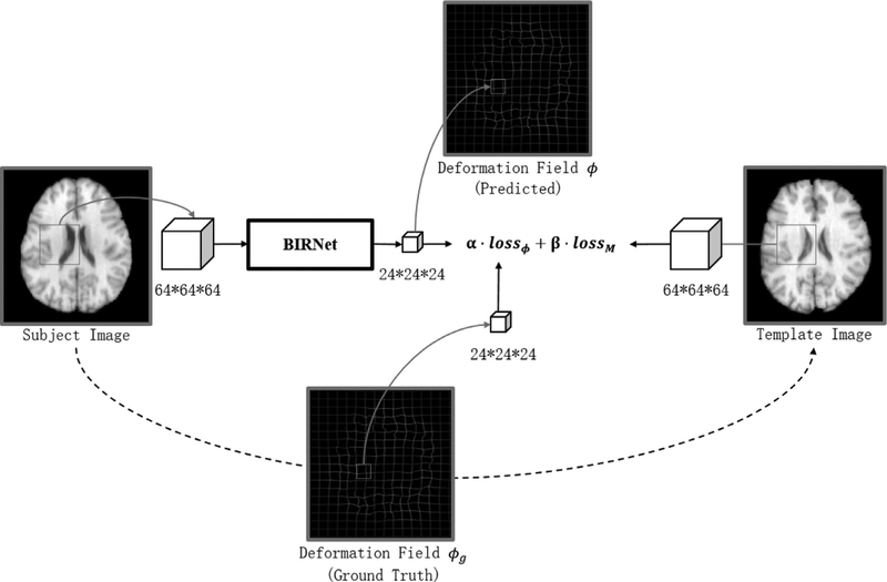
In our dual-guidance strategy, the loss function consists of two parts: 1) loss_ϕ—the difference between the predicted deformation field and the existing (training) ground-truth deformation field; 2) loss_M —the difference between the template and the warped subject image based on the deformation currently estimated via the network.

Here, loss_ϕ is the Euclidean distance as defined in (Rohé et al., 2017; Sokooti et al., 2017), which assumes that the ground-truth deformation fields are already achieved. As shown in Fig. 2, for the template image T and subject image S, the ground-truth deformation field ϕ_g is used to guide the training of the deep learning model with loss function:

$$los{s}_{\varphi }=\frac{1}{N}\Vert \varphi -{\varphi }_g{\Vert }_2^2$$ (2)

where ϕ is the predicted deformation field and N is the number of voxels. Note that the performance of trained model is limited by the ground-truth deformation fields, which are obtained using traditional registration methods before training (Avants et al., 2008; Vercauteren et al., 2009). To improve accuracy, we include the following loss function:

$$los{s}_M=\frac{1}{N}\sum _u\Vert S(u+\varphi (u))-T(u){\Vert }_2^2$$ (3)

where u represents the voxel coordinate [x, y, z] in the template space and ϕ(u) = [d_x, d_y, d_z] is the displacement of u. Specifically, loss_ϕ indicates the difference of the predicted displacement and the ground-truth displacement, so the range of meaningful gradient is [−30, 30] (which can well cover the potential displacement magnitude); loss_M measures the difference of the image intensity, so the range of meaningful gradient is [−255, 255] (since the original image intensity range is 0–255). In order to normalize the two losses, the gradient of loss_M has been multiplied by 0.1 in the actual implementation. Then, by combining the ground-truth loss function loss_ϕ and the dissimilarity loss function loss_M together, the final loss function is

$$loss=\alpha \cdot los{s}_{\varphi }+\beta \cdot los{s}_M,\alpha +\beta =1$$ (4)

where α and β are the two coefficients satisfying α≥ 0, β≥ 0, and α+β = 1. They are dynamically varied during the training process, i.e., taking a larger α (learn more from ground truth) in the initial training stage to accelerate convergence and achieve smooth deformation fields, then taking a larger β-value (learn more from image dissimilarity) in the later fine-tuning stage to further refine the registration. In actual implementation, we set α= 0.8 and β = 0.2 in the initial training stage (i.e., the first 5 epochs), and α= 0.5 and β = 0.5 in the later training stage (i.e., the last 5 epochs). However, a lower α is not recommended, because the predicted deformation field will not be able to keep smooth and regular without the constraint of loss_ϕ.

Fig. 2.

Training strategy with loss function α · loss_ϕ + β · loss_M.

Specifically, the loss function works by giving the gradient value backward to the front layers. Let [d_x, d_y, d_z] consist of a vector of displacements. Then, the gradient in x-direction can be represented by the following equation:

$$\begin{gathered} \frac{\partial {\text{loss}}_M}{\partial dx}=\frac{M(dx+\mathrm{\Delta }dx)-M(dx)}{\mathrm{\Delta }dx} \\ =\begin{array}{l}\left|S(x+dx+1,y+dy,z+dz)-T(x,y,z)\right|\hfill \\ -\left|S(x+dx,y+dy,z+dz)-T(x,y,z)\right|\hfill \end{array} \end{gathered}$$ (5)

where we calculate an error in recent vector first, and then plus one in the recent direction x and calculate the varying error. Finally, the difference between them will be the gradient. The gradient of d_y and d_z could be calculated in the same way.

In summary, using dual-guidance can effectively combine the advantages of both loss functions: (1) the rough guidance provided by loss_ϕ makes the convergence easily and fast; and (2) the image difference guidance provided by loss_M further refines the registration results, which can address the issue of inaccurate ground truth.

3.2.1.2. Hierarchical supervision.

In the conventional U-Net, the loss is calculated only in the final layer, resulting in suboptimal parameters in the frontal convolution layers (Schmidhuber, 2015). In this way, the parameters of the first half of the convolution layers are not updated as much as the latter half. This not only causes slow convergence, but also causes the over-fitting problem. Therefore, we add a loss function in each of the layers to directly supervise the training of the first (frontal) half of the network.

As we use filters with size 3 × 3 × 3, each convolutional layer without padding reduces the patch size isotropically by one voxel. Also, each pooling layer will further downsample the patch. As a result, for an input patch size of 64 × 64 × 64, we extract 24 × 24 × 24 patch ${\varphi }_g^{high}$ for high resolution, 14 × 14 × 14 patch ${\varphi }_g^{mid}$ for middle resolution, and 9 × 9 × 9 patch ${\varphi }_g^{low}$ for low resolution. The translations from ϕ_g to ${\varphi }_g^{high}$, ${\varphi }_g^{mid}$, ${\varphi }_g^{low}$ are:

$$\begin{gathered} {\varphi }_g^{high}(i,j,k)={\varphi }_g(i+20,j+20,k+20) \\ i,j,k\in [0,23] \\ {\varphi }_g^{mid}(i,j,k)={\varphi }_g(i\times 2+18,j\times 2+18,k\times 2+18)/2 \\ i,j,k\in [0,13] \\ {\varphi }_g^{low}(i,j,k)={\varphi }_g(i\times 4+14,j\times 4+14,k\times 4+14)/4 \\ i,j,k\in [0,8] \end{gathered}$$ (6)

where i, j, k are the coordinates of the points in the patch. Then, we can easily calculate the respective loss function for each level as:

$$\begin{gathered} los{s}_{\varphi }^{high}=\frac{1}{24\times 24\times 24}\Vert {\varphi }^{high}-{\varphi }_g^{high}{\Vert }_2^2 \\ los{s}_{\varphi }^{mid}=\frac{1}{14\times 14\times 14}\Vert {\varphi }^{mid}-{\varphi }_g^{mid}{\Vert }_2^2 \\ los{s}_{\varphi }^{low}=\frac{1}{9\times 9\times 9}\Vert {\varphi }^{low}-{\varphi }_g^{low}{\Vert }_2^2 \end{gathered}$$ (7)

where ϕ^high, ϕ^mid, ϕ^low are predicted by the learning model directly, which are in the same size as ϕ_g^high, ϕ_g^mid, ϕ_g^low. Finally, the total loss function loss_ϕ is:

$$los{s}_{\varphi }=los{s}_{\varphi }^{high}+los{s}_{\varphi }^{mid}+los{s}_{\varphi }^{low}$$ (8)

3.2.2. Gap filling

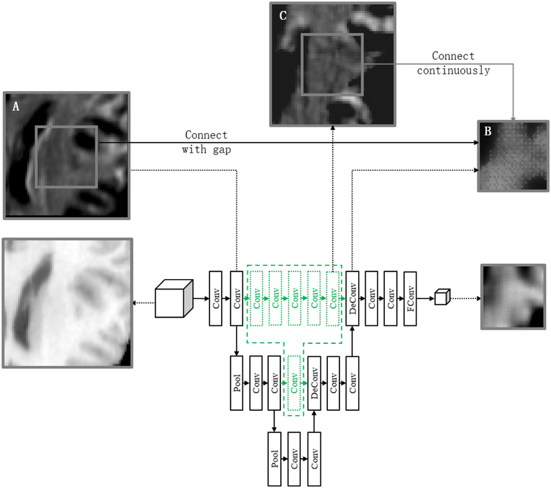
The black network in Fig. 3 is the basic network architecture of U-Net. It consists of a contracting path (left side) and an expansive path (right side). The contracting path follows the typical architecture of a convolutional network. It consists of repeated applications of two 3 × 3 × 3 convolutions (i.e., convolutions that may be followed by ReLU (He et al., 2015), and batch normalization layers (Ioffe and Szegedy, 2015)), and a 2 × 2 × 2 max pooling operation with stride size of 2 for downsampling. At each downsampling step, we double the number of feature channels. Every step in the expansive path consists of a 2 × 2 × 2 deconvolution to upsample the feature map and half the number of feature channels, and also two 3 × 3 × 3 convolutions. At the final layer, a 1 × 1 × 1 convolution is used to map each 64-component feature vector to the desired number of channels. To recover detail lost due to downsampling, we concatenate the correspondingly cropped feature map from the contracting path.

Fig. 3.

The feature image samples of the typical layers in the network. The output deformation field is shown by the feature image of the displacement value in x-axial.

As shown in Fig. 3, two feature maps A and B are significantly dissimilar. Feature map A resembles the original image, whereas feature map B resembles the deformation field. Obviously, there is a huge gap between the feature maps A and B, which are usually concatenated together by the conventional U-Net. This gap makes the network less effective in both training and testing stages for this regression task. It is worth noting that, the feature map is an intermediate feature map which is up-sampled from the low-level feature map by deconvolution, hence adjacent voxels may refer to different information. Therefore, feature map B looks a little discontinuous.

To address this issue, we propose to include additional convolution layers between the same level of the contracting phase and the expansion phase (as shown by the green network in Fig. 3) to synchronize the convolution path of the feature maps. The parameters of the added convolution layers are equal to the convolution layers in the lower resolution. In this way, the feature map C after gap filling will be more similar to the feature map B, improving both registration accuracy and training speed.

3.2.3. Multi-channel inputs

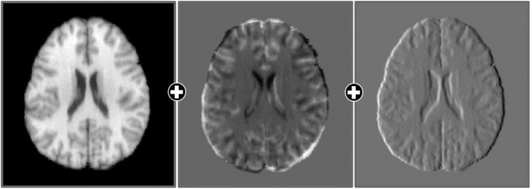
Image feature maps, such as difference and gradient maps, can also be used to improve registration accuracy. Fig. 4 shows the multi-channel inputs, including the original image, difference map, and gradient map. The difference map is computed as the intensity difference between the subject and template images. The gradient map provides boundary information to help structural alignment. Moreover, gradient maps, in addition to the intensity images, are used to calculate the image similarity in Eq. (3). This ensures that the boundaries can be aligned more accurately. Note that the gradient maps are scaled to the same value range of the intensity images for consistent comparison. Usually, deep learning network can learn the required features by itself. However, the loss functions are usually calculated only in the final layer, resulting in suboptimal parameters in the frontal convolution layers (Schmidhuber, 2015). Therefore, inputting the gradient map and difference map, which are shown to be useful in conventional registration methods, from the beginning can largely increase the effect of the parameters in the frontal convolution layers and the convergence speed.

Fig. 4.

The concatenated original image, difference map, and gradient map.

3.2.4. Implementation

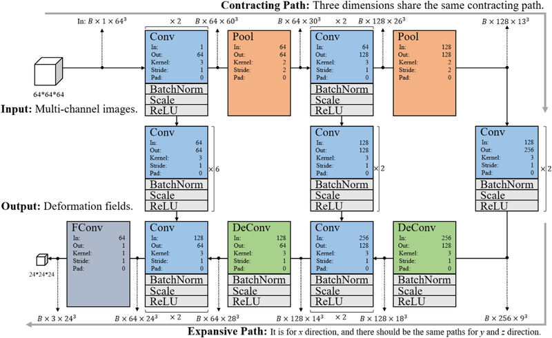
Fig. 5 shows the architecture of the proposed 3D image registration network, which is based on the 64 × 64 × 64 input patches of image appearance and the 24 × 24 × 24 output patches of deformation. The network is implemented using 3D Caffe (Jia et al., 2014) and optimized using Adam (Kingma and Ba, 2014). We set the learning rate to 1e-3 for the initial training stage and 1e-8 for the fine-tuning training stage. The network takes one 3D patch from the subject image as the input, and outputs one 3D deformation field patch, which consists of three independent patches for the x, y and z dimensions, respectively (note that only one branch is shown in Fig. 5).

Fig. 5.

The architecture of image registration network. Conv: 3D convolution layer. Pool: 3D pooling layer. DeConv: Deconvolution layer. BatchNorm: Batch normalization layer. Scale: Scale layer. ReLU: ReLU layer. In: The number of input channels. Out: The number of output channels. Kernel: The kernel size of the 3D filter in each dimension. Stride: Stride of the 3D filter. Pad: Zero-padding. B: Batch size.

The patches have overlaps during sampling in the training stage. Basically, the input patch size is 64 × 64 × 64, the output deformation patch size is 24 × 24 × 24, which is corresponding to the center region of the input patch. When training or applying the network for the whole images, we extract overlapping patches by the step size of 24, i.e., the output patch size. Thus, all the non-overlapping output patches can form the whole deformation field.

3.3. Data augmentation

We evaluate our method on 3D brain MR images. We use LONI LPBA40 (Shattuck et al., 2008) dataset (image size: 220 × 220 × 184) for training, where we choose one image as the template, 30 images as the training images, and the remaining 9 images as the validation images. Since it is difficult to judge which registration result is closer to the ground truth, we employ two ground-truths generated by both ANTs (Avants et al., 2008) and LCC-Demons (Lorenzi et al., 2013) to each subject, i.e., in training data each subject occurs twice with two different labels.

We augment the dataset because it is too small for effective training. This is done by warping each subject image with 20%, 40%, 60%, 80%, and 100% of the ground-truth deformation, mean-while, the respective deformation field is the target of prediction. An example is shown in Fig. 6. It works because the deep learning model does not iteratively calculate the deformation field, and thus the intermediate results with different degrees of deformation are effective samples for deep network training. This significantly expands the size of training dataset by 6 folds and will allow coarse and fine deformations to participate in the training.

Fig. 6.

Expanded training data constructed by warping the subject image with varying degrees.

4. Experiments

To evaluate the performance of our proposed method, the comparison with several state-of-the-art deformable registration algorithms is shown in this section. We train BIRNet using LPBA40 (Shattuck et al., 2008) dataset, where the 1st image in LPBA40 is chosen as template image, 1–30th images as training samples, and 31–40th image as validation data. Then we directly apply it to four different testing datasets without refinement, including IBSR18 (Klein et al., 2009), CUMC12 (Klein et al., 2009), MGH10 (Klein et al., 2009), and IXI30 (Serag et al., 2012). In preprocessing, all the subjects are linearly registered to the template space by using FLIRT (Jenkinson and Smith, 2001). Dice Similarity Coefficient (DSC) is used to evaluate the registration performance based on the ROIs labels.

We select 4 state-of-the-art registration methods (Klein et al., 2009), i.e., Diffeomorphic Demons (Vercauteren et al., 2009), LCC-Demons (Lorenzi et al., 2013), FNIRT (Andersson et al., 2007), and SyN (Avants et al., 2008), for comparison. All the competing methods including different training strategies are briefly introduced as follows.

1. Diffeomorphic Demons (Vercauteren et al., 2009): An efficient non-parametric image registration algorithm, which introduces diffeomorphisms into the demons framework.

2. LCC-Demons (Lorenzi et al., 2013): A fast and robust registration framework based on the log-Demons diffeomorphic registration algorithm. The transformation is parameterized by stationary velocity fields, and the similarity metric implements a symmetric local correlation coefficient (LCC).

3. FNIRT (Andersson et al., 2007): A widely used registration tool in FSL. The registration is based on a weighted sum of scaled sum-of-squared differences and membrane energy.

4. SyN (Avants et al., 2008): A symmetric image normalization method (SyN) for maximizing the cross-correlation within the space of diffeomorphic maps and providing the Euler-Lagrange equations necessary for this optimization.

5. U-Net (Ronneberger et al., 2015): The original U-Net is a typical encoder-decoder-architecture-based FCN model with skip connections. We use the ground-truth deformations obtained by LCC-Demons and SyN to train U-Net on image registration. For a fair comparison, all the training settings are consistent with those of the proposed method.

6. BIRNet_WOS: In this model, we add the hierarchical supervision, gap filling, and multichannel inputs based on the U-Net. This model is still supervised by ground-truth guidance, without image dissimilarity guidance.

7. BIRNet: The same setting as BIRNet-WOS but with dual-guidance (our proposed method).

4.1. Evaluation based on LPBA40

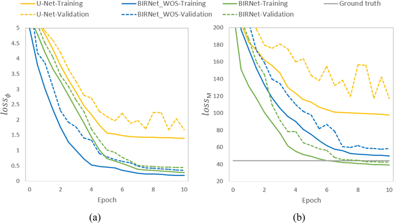
We test the performance of BIRNet on LPBA40 dataset. For each of the 180 training images, we extract 300 patches of size 64 × 64 × 64, giving us a total of 54,0 0 0 training patches. Fig. 7 shows the loss curves of loss_ϕ and loss_M for both training and validation. From Fig. 7 (a) we can see that the performance of U-Net saturates fast during training. BIRNet_WOS improves the performance on both convergence speed and the ability to overcome over-fitting, benefiting from the combined effects of hierarchical supervision, gap filling and multichannel inputs. We further compare the effect of each strategy and show the respective performance in Table 1, where we quantitatively compare the memory occupied, computational time of each iteration, and the DSC calculated on 54 brain ROIs. Compared to the U-Net structure, the gap filling strategy increases some memory load and computational time due to the additional convolutional layers. Besides this, all these three strategies improve the registration performance without adding too much extra computing burden.

Fig. 7.

The training and validation curves for (a) loss_ϕ and (b) loss_M. The value of loss_ϕ is shown as the mean square error of displacement, whereas the value of loss_M is shown as the mean square error of intensity.

Table 1.

Evaluation results for the separate effects of the proposed training strategies hierarchical supervision (HS), gap filling (GF), multi-channel inputs (MI), and dual-supervision (DS).

	Methods	Avg.	Std.
Memory occupied (Mb)	U-Net	4786	-
	U-Net+HS	4789	-
	U-Net+HS+GF	6437	-
	U-Net+HS+GF+MI (BIRNet_WOS)	6438	-
	BIRNet_WOS+DS (BIRNet)	6438	-
Avg. training time of each iteration (s)	U-Net	0.24	0.08
	U-Net+HS	0.25	0.07
	U-Net+HS+GF	0.27	0.08
	U-Net+HS+GF+MI (BIRNet_WOS)	0.27	0.08
	BIRNet_WOS+DS (BIRNet)	0.38	0.09
Avg. DSC of training set (%)	U-Net	65.3	2.4
	U-Net+HS	67.4	2.1
	U-Net+HS+GF	68.2	1.9
	U-Net+HS+GF+MI (BIRNet_WOS)	68.9	1.9
	BIRNet_WOS+DS (BIRNet)	69.8	1.8
Avg. DSC of validation set (%)	U-Net	64.4	2.8
	U-Net+HS	65.8	2.3
	U-Net+HS+GF	66.3	2.4
	U-Net+HS+GF+MI (BIRNet_WOS)	66.7	2.0
	BIRNet_WOS+DS (BIRNet)	69.2	2.1

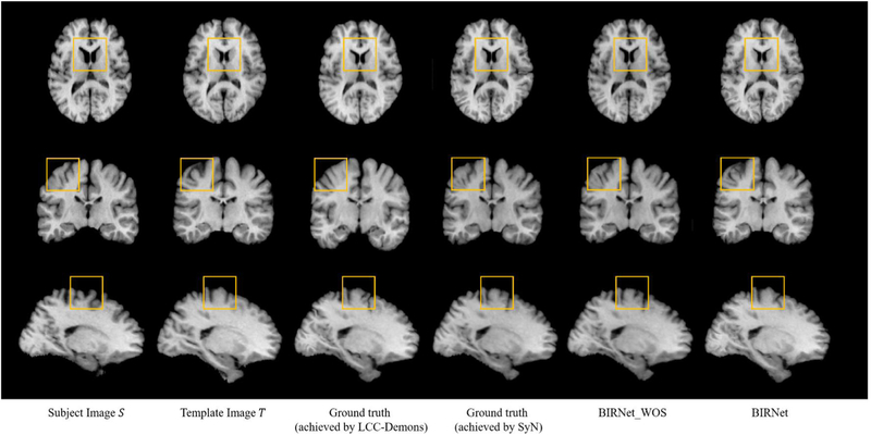
Additionally, in both Fig. 7 (a) and Table 1, the best performance for the training set is given by BIRNet, which further considers image similarity/difference. The BIRNet model has reached a lower dissimilar score even than the ground truth for the validation set in Fig. 7 (b). These results demonstrate that the image similarity/difference loss can provide useful guidance to further refine the training model, even the ground-truth deformation fields cannot be quite accurate. Fig. 8 shows an example of the registration results, confirming that the results obtained by BIRNet are most similar to the template, especially in the yellow squared regions.

Fig. 8.

An example of the registration outcomes. Improvements are marked by yellow boxes.

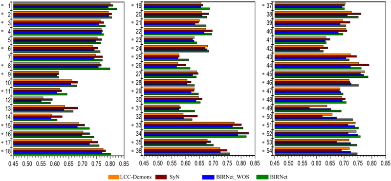
Fig. 9 shows the Dice similarity coefficient (DSC) of 54 brain ROIs (with the ROI names give in Table 2, obtained from (Shattuck et al., 2008)). We observe that BIRNet yields better performance for 35 out of 54 ROIs and the comparable performance for the other 19 ROIs with LCC-Demons and SyN. BIRNet_WOS shows accuracy that is a little worse than LCC-Demons and SyN, which shows that the dual-guidance is effective in boosting the performance. Since the proposed method does not need very accurate ground-truth deformations for training, the unseen testing dataset can be easily used to refine the trained model. Therefore, the performance on the training data also indicates the expected performance that the proposed model can achieve after fully refinement for unseen testing datasets.

Fig. 9.

The mean DSCs of 54 ROIs based on 30 training subjects from the LPBA40 dataset, after deformable registration by LCC-Demons, SyN, BIRNet_WOS and BIRNet. “*” marks the cases where BIRNet achieves the highest DSC value among all the four methods.

Table 2.

The names of the ROIs in LONI LPBA40 (Shattuck et al., 2008) dataset.

ID	Fullname	ID	Fullname	ID	Fullname
1	L superior frontal gyrus	19	L supramarginal gyrus	37	L inferior temporal gyrus
2	R superior frontal gyrus	20	R supramarginal gyrus	38	R inferior temporal gyrus
3	L middle frontal gyrus	21	L angular gyrus	39	L parahippocampal gyrus
4	R middle frontal gyrus	22	R angular gyrus	40	R parahippocampal gyrus
5	L inferior frontal gyrus	23	L precuneus	41	L lingual gyrus
6	R inferior frontal gyrus	24	R precuneus	42	R lingual gyrus
7	L precentral gyrus	25	L superior occipital gyrus	43	L fusiform gyrus
8	R precentral gyrus	26	R superior occipital gyrus	44	R fusiform gyrus
9	L middle orbitofrontal gyrus	27	L middle occipital gyrus	45	L insular cortex
10	R middle orbitofrontal gyrus	28	R middle occipital gyrus	46	R insular cortex
11	L lateral orbitofrontal gyrus	29	L inferior occipital gyrus	47	L cingulate gyrus
12	R lateral orbitofrontal gyrus	30	R inferior occipital gyrus	48	R cingulate gyrus
13	L gyrus rectus	31	L cuneus	49	L caudate
14	R gyrus rectus	32	R cuneus	50	R caudate
15	L postcentral gyrus	33	L superior temporal gyrus	51	L putamen
16	R postcentral gyrus	34	R superior temporal gyrus	52	R putamen
17	L superior parietal gyrus	35	L middle temporal gyrus	53	L hippocampus
18	R superior parietal gyrus	36	R middle temporal gyrus	54	R hippocampus

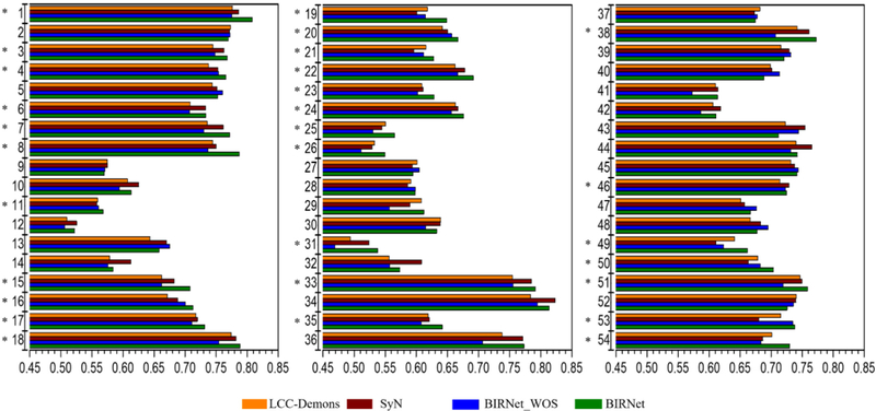
Fig. 10 shows the DSC results for 9 validation subject images from LPBA40. BIRNet_WOS results in a slight performance drop compared with LCC-Demons and SyN, but only by a small extent (i.e., less than 1.5% in average). BIRNet again achieves the best performance with higher DSC values on 29 out of 54 ROIs and very similar values on the other 25 ROIs compared with LCC-Demons and SyN. The average DSC of LCC-Demons, SyN, BIRNet_WOS and BIRNet are 67.9%, 68.1%, 67.0% and 69.2%, respectively. These results verify the generalizability of BIRNet.

Fig. 10.

The mean DSC of 54 ROIs based on 9 validation subjects from LPBA40 dataset, after deformable registration by LCC-Demons, SyN, BIRNet_WOS and BIRNet. “*” marks the cases where BIRNet achieves the highest DSC value among all the four methods.

4.2. Evaluation based on IBSR18, CUMC12, MGH10, IXI30

To further evaluate the accuracy and generalizability of BIRNet, we further test it on a total of 70 brain images from four different datasets, i.e., IBSR18 (Klein et al., 2009), CUMC12 (Klein et al., 2009), MGH10 (Klein et al., 2009), and IXI30 (Serag et al., 2012), by directly applying the model trained using the LPBA40 dataset without any additional parameter tuning. The results for one subject of the IBSR18 dataset is shown in Fig. 11 for Diffeomorphic Demons, LCC-Demons, SyN, FNIRT (Andersson et al., 2007) and BIRNet. Note that, the results shown for SyN and FNIRT are based on their optimal parameters determined individually for each image. Table 3 provides the DSCs for of Gray Matter (GM) and White Matter (WM) based on GM and WM labels provided in these four datasets. The performance of BIRNet is comparable to the fine-tuned SyN and FNIRT (particularly to each of these four datasets), but without the need for parameter tuning. This verifies the generalizability of BIR-Net.

Fig. 11.

Example testing case in IBSR18 dataset.

Table 3.

Results for IBSR18, CUMC12, MGH10, IXI30 in term of DSC (%). Results for both default and tuned parameters are shown for FNIRT and SyN.

Dataset	Brain Tissue	Affine	D.Demons	LCC-Demons	FNIRT	FNIRT (default)	SyN	SyN (default)	BIRNet
IBSR18	GM	65.4 ± 3.4	73.7 ± 2.4	74.4 ± 1.7	74.3 ± 1.8	73.1 ± 2.3	73.9 ± 2.2	72.9 ± 2.8	74.2 ± 2.2
	WM	61.7 ± 2.5	75.8 ± 1.5	76.8 ± 1.5	76.5 ± 2.0	75.1 ± 1.9	77.6 ± 1.7	75.2 ± 2.3	77.0 ± 2.1
CUMC12	GM	57.2 ± 4.2	74.6 ± 2.2	74.9 ± 2.1	74.4 ± 2.4	73.4 ± 3.1	75.1 ± 1.8	73.2 ± 3.4	74.3 ± 2.5
	WM	58.1 ± 4.0	75.5 ± 2.0	76.8 ± 1.7	76.3 ± 1.5	74.9 ± 2.0	76.7 ± 1.2	74.3 ± 2.2	76.7 ± 1.3
MGH10	GM	61.7 ± 4.5	73.1 ± 3.4	73.3 ± 2.9	74.1 ± 2.8	73.1 ± 3.1	73.6 ± 2.3	72.8 ± 4.1	73.8 ± 2.4
	WM	61.2 ± 3.3	78.3 ± 1.6	78.7 ± 2.2	78.8 ± 2.1	77.9 ± 2.5	79.1 ± 1.9	77.7 ± 2.8	79.7 ± 1.6
IXI30	GM	61.6 ± 3.8	72.4 ± 2.5	74.1 ± 2.1	74.4 ± 2.4	72.7 ± 2.5	75.2 ± 1.6	71.6 ± 2.9	74.7 ± 2.2
	WM	61.4 ± 3.4	76.9 ± 1.9	77.9 ± 1.7	78.1 ± 2.0	77.4 ± 2.7	78.3 ± 1.7	76.5 ± 3.0	77.7 ± 1.8

4.3. Regularization analysis

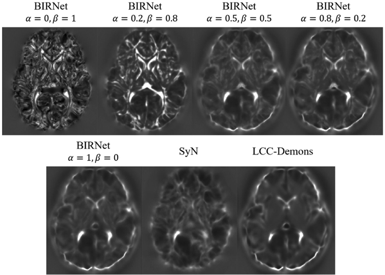
The smooth and diffeomorphic deformation fields given by LCC-Demons and SyN can provide guidance for deformation regularization. By balancing between loss_ϕ and loss_M, the predicted deformation fields are encouraged to be both smooth and regular. To verify this, we show the Jacobian determinant map of the predicted deformation fields in Fig. 12. From the figure, we can see that, the proposed BIRNet, which is supervised only by ground truth (α= 1, β = 0), keeps the smoothness of the ground-truth deformation. If BIRNet is trained only supervised by the image dissimilarity metric (α= 1, β = 0), the output deformation field is quite noisy. When we set α= 0.5, β = 0.5, the predicted deformation field almost maintains the smoothness and balances the two loss functions. Therefore, since we have a strong guidance from the smooth ground-truth deformation fields, we can ensure the smoothness even without an additional regularization constraint.

Fig. 12.

The changes of Jacobian determinants with the balancing coefficients between loss_ϕ and loss_M. BIRNet with α = 1, β = 0 is supervised only by the ground-truth achieved by SyN and LCC-Demons; BIRNet with α = 0, β = 1 is supervised only by the image dissimilarity metric; BIRNet with α = 0.8, β = 0.2 is trained in the initial training stage (i.e., the first 5 epochs), and BIRNet with α = 0.5, β = 0.5 is trained in the fine-tuning stage.

4.4. Computation costs

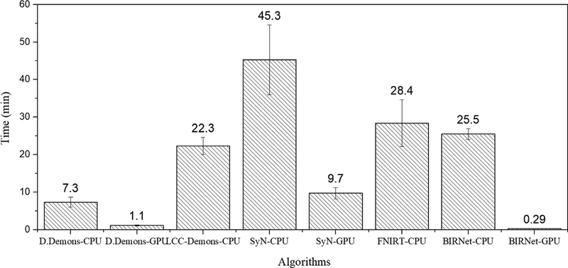
BIRNet is implemented based on Caffe (Jia et al., 2014) on a single Nvidia TitanX (Pascal) GPU. For a fair comparison, we compare its speed with CPU and GPU implementations of other comparison methods. (Note that there is no GPU implementation for LCC-Demons (Lorenzi et al., 2013) and FNIRT (Fluck et al., 2011)). Fig. 13 shows the computation costs for a typical 3D brain image (220 × 220 × 184) of eight different deformable registration algorithms: Diffeomorphic Demons–CPU (Vercauteren et al., 2009), Diffeomorphic Demons—GPU (Muyan-Ozcelik et al., 2008), LCC-Demons—CPU (Lorenzi et al., 2013), SyN—CPU (Avants et al., 2008), SyN—GPU (Luo et al., 2015), FNIRT—CPU (Andersson et al., 2007), BIRNet—CPU, and BIRNet—GPU. It is clear that BIRNet, which does not require any iterative optimization, shows a huge boost when implemented on GPU and requires the least amount of time.

Fig. 13.

Average computational times (in minutes) of different registration algorithms for registering a 220 × 220 × 184 brain image.

5. Discussion

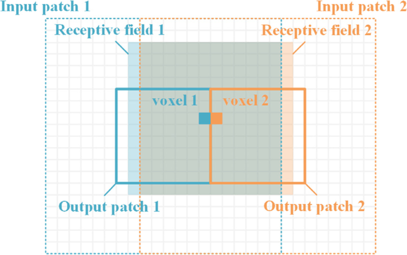
Our model is able to predict the deformation of a template image towards a subject image based on the slicing patches, and then concatenate all the patches to form the whole deformation field. Therefore, some adjacent voxels at patch boundaries will be computed in different patches, which seems to be discontinuous. However, it is well known that the predicted value of each voxel in a convolutional neural network is only affected by its receptive field. The receptive fields of adjacent voxels are continuous, even if they are in different patches, as shown in Fig. 14. Consequently, the deformation continuity at patch boundaries can be ensured in this framework.

Fig. 14.

Schematic diagram of the continuity of the adjacent voxels at patch bound-aries.

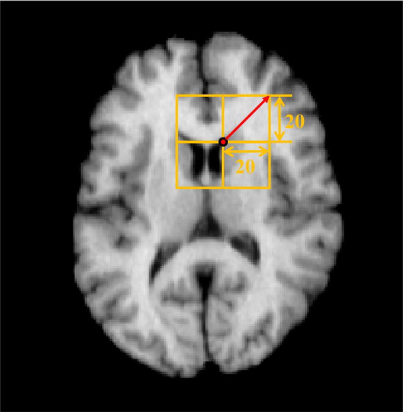
As mentioned, the predicted displacement vector of a voxel is affected by its receptive field. The size of the receptive field is 41 × 41 × 41 in the proposed model, based on the number of convolutional and pooling layers. Therefore, the maximum offset of displacement vector in each direction is 20, which is sufficient for measuring the local deformations, as indicated in Fig. 15. When dealing with larger scale deformed images, the range of receptive field needs to be enlarged by adding more convolutional and pooling layers.

Fig. 15.

Sample of the range of maximum displacement in the model.

The proposed network focuses on registering the subject image to a fixed template image, because registering images to a same template image is an important preprocessing component of most medical image analysis methods, e.g., atlas alignment. When transferring to a new reference image, the well-trained model can be refined with a limited number of training samples instead of retraining from scratch. The current network is proposed for brain MR image registration, but it has the potential to extend to other organs and even multimodal image registration problems. For multimodal image registration, SSD loss should be computed on the mutual information images or be directly replaced by cross-correlation loss.

6. Conclusion

In this paper, we have introduced a dual-guided fully convolutional neural network, called BIRNet. To solve the issue of lacking ground-truth problem, BIRNet uses both pre-registered ground-truth deformation field and image similarity/difference metric to guide the training stage, thus making the deep learning model able to further refine the results. BIRNet employs strategies such as gap filling, hierarchical supervision, multi-channel inputs, and aries. data augmentation for improving registration accuracy. Experimental results indicate that BIRNet achieves the state-of-the-art performance without the need for parameter tuning. In summary, since the proposed BIRNet method is a fast, accurate, and easy-to-use method for brain image registration, it could be directly applied to many practical registration problems.

References

- Andersson JL, Jenkinson M, Smith S, 2007. Non-linear registration, aka Spatial normalisation FMRIB technical report TR07JA2. FMRIB Analysis Group of the University of Oxford; 2. [Google Scholar]
- Auzias G, Colliot O, Glaunes JA, Perrot M, Mangin J-F, Trouve A, Baillet S, 2011. Diffeomorphic brain registration under exhaustive sulcal constraints. IEEE Trans. Med. Imaging 30, 1214–1227. [DOI] [PubMed] [Google Scholar]
- Avants BB, Epstein CL, Grossman M, Gee JC, 2008. Symmetric diffeomorphic image registration with cross-correlation: evaluating automated labeling of elderly and neurodegenerative brain. Med. Image Anal. 12, 26–41. [DOI] [PMC free article] [PubMed] [Google Scholar]
- Balakrishnan G, Zhao A, Sabuncu MR, Guttag J, Dalca AV, 2018. An unsupervised learning model for deformable medical image registration. In: Proceedings of the IEEE Conference on Computer Vision and Pattern Recognition, pp. 9252–9260. [Google Scholar]
- Balakrishnan G, Zhao A, Sabuncu MR, Guttag J, Dalca AV, 2019. VoxelMorph: a learning framework for deformable medical image registration. IEEE Trans. Med. Imaging [DOI] [PubMed] [Google Scholar]
- Cao T, Singh N, Jojic V, Niethammer M, 2015. Semi-coupled dictionary learning for deformation prediction, Biomedical Imaging (ISBI) In: 2015 IEEE 12th International Symposium on. IEEE, pp. 691–694. [Google Scholar]
- Cao X, Yang J, Zhang J, Nie D, Kim M, Wang Q, Shen D, 2017. Deformable image registration based on similarity-steered cnn regression In: International Conference on Medical Image Computing and Computer-Assisted Intervention. Springer, pp. 300–308. [DOI] [PMC free article] [PubMed] [Google Scholar]
- Dosovitskiy A, Fischer P, Ilg E, Hausser P, Hazirbas C, Golkov V, Van Der Smagt P, Cremers D, Brox T, 2015. Flownet: learning optical flow with convolutional networks. In: Proceedings of the IEEE International Conference on Computer Vision, pp. 2758–2766. [Google Scholar]
- Fan J, Yang J, Ai D, Xia L, Zhao Y, Gao X, Wang Y, 2016a. Convex hull indexed Gaussian mixture model (CH-GMM) for 3D point set registration. Pattern Recognit. 59, 126–141. [Google Scholar]
- Fan J, Yang J, Lu F, Ai D, Zhao Y, Wang Y, 2016b. 3-points convex hull matching (3PCHM) for fast and robust point set registration. Neurocomputing 194, 227–240. [Google Scholar]
- Fan J, Yang J, Zhao Y, Ai D, Liu Y, Wang G, Wang Y, 2017. Convex hull aided registration method (CHARM). IEEE Trans. Vis. Comput. Graph 23, 2042–2055. [DOI] [PubMed] [Google Scholar]
- Fluck O, Vetter C, Wein W, Kamen A, Preim B, Westermann R, 2011. A survey of medical image registration on graphics hardware. Comput. Methods Programs Biomed. 104, e45–e57. [DOI] [PubMed] [Google Scholar]
- Gutiérrez-Becker B, Mateus D, Peter L, Navab N, 2016. Learning optimization updates for multimodal registration In: International Conference on Medical Image Computing and Computer-Assisted Intervention. Springer, pp. 19–27. [Google Scholar]
- Gutierrez-Becker B, Mateus D, Peter L, Navab N, 2017. Guiding multimodal registration with learned optimization updates. Med. Image Anal 41, 2–17. [DOI] [PubMed] [Google Scholar]
- He K, Zhang X, Ren S, Sun J, 2015. Delving deep into rectifiers: surpassing human-level performance on imagenet classification. In: Proceedings of the IEEE international conference on computer vision, pp. 1026–1034. [Google Scholar]
- Hu Y, Modat M, Gibson E, Ghavami N, Bonmati E, Moore CM, Emberton M, Noble JA, Barratt DC, Vercauteren T, 2018. Label-driven weakly-supervised learning for multimodal deformarle image registration, Biomedical Imaging (ISBI 2018) In: 2018 IEEE 15th International Symposium on. IEEE, pp. 1070–1074. [Google Scholar]
- Ilg E, Mayer N, Saikia T, Keuper M, Dosovitskiy A, Brox T, 2017. Flownet 2.0: evolution of optical flow estimation with deep networks. In: IEEE conference on computer vision and pattern recognition (CVPR), p. 6. [Google Scholar]
- Ioffe S, Szegedy C, 2015. Batch normalization: accelerating deep network training by reducing internal covariate shift. In: International Conference on Machine Learning, pp. 448–456. [Google Scholar]
- Jenkinson M, Smith S, 2001. A global optimisation method for robust affine registration of brain images. Med. Image Anal. 5, 143–156. [DOI] [PubMed] [Google Scholar]
- Jia Y, Shelhamer E, Donahue J, Karayev S, Long J, Girshick R, Guadarrama S, Darrell T, 2014. Caffe: convolutional architecture for fast feature embedding In: Proceedings of the 22nd ACM international conference on Multimedia. ACM, pp. 675–678. [Google Scholar]
- Johnson HJ, Christensen GE, 2002. Consistent landmark and intensity-based image registration. IEEE Trans. Med. Imaging 21, 450–461. [DOI] [PubMed] [Google Scholar]
- Kim M, Wu G, Wang Q, Lee S-W, Shen D, 2015. Improved image registration by sparse patch-based deformation estimation. NeuroImage 105, 257–268. [DOI] [PMC free article] [PubMed] [Google Scholar]
- Kim M, Wu G, Yap P-T, Shen D, 2012. A general fast registration framework by learning deformation–appearance correlation. IEEE Trans. Image Process 21, 1823–1833. [DOI] [PMC free article] [PubMed] [Google Scholar]
- Kingma D, Ba J, 2014. Adam: a method for stochastic optimization. arXiv:1412.6980. [Google Scholar]
- Klein A, Andersson J, Ardekani BA, Ashburner J, Avants B, Chiang M-C, Christensen GE, Collins DL, Gee J, Hellier P, 2009. Evaluation of 14 nonlinear deformation algorithms applied to human brain MRI registration. NeuroImage 46, 786–802. [DOI] [PMC free article] [PubMed] [Google Scholar]
- Klein S, Staring M, Murphy K, Viergever MA, Pluim JP, 2010. Elastix: a tool-box for intensity-based medical image registration. IEEE Trans. Med. Imaging 29, 196–205. [DOI] [PubMed] [Google Scholar]
- Krebs J, e Delingette H, Mailhé B, Ayache N, Mansi T, 2019. Learning a probabilistic model for diffeomorphic registration. IEEE Trans. Med. Imaging [DOI] [PubMed] [Google Scholar]
- Krebs J, Mansi T, Delingette H, Zhang L, Ghesu FC, Miao S, Maier AK, Ayache N, Liao R, Kamen A, 2017. Robust non-rigid registration through agent-based action learning In: International Conference on Medical Image Computing and Computer-Assisted Intervention. Springer, pp. 344–352. [Google Scholar]
- Loeckx D, Maes F, Vandermeulen D, Suetens P, 2003. Non-rigid image registration using a statistical spline deformation model In: Biennial International Conference on Information Processing in Medical Imaging. Springer, pp. 463–474. [DOI] [PubMed] [Google Scholar]
- Lorenzi M, Ayache N, Frisoni GB, Pennec X, Initiative, A.s.D.N., 2013. LC-C-Demons: a robust and accurate symmetric diffeomorphic registration algorithm. NeuroImage 81, 470–483. [DOI] [PubMed] [Google Scholar]
- Luo Y. g., Liu P, Shi L, Luo Y, Yi L, Li A, Qin J, Heng P-A, Wang D, 2015. Accelerating neuroimage registration through parallel computation of similarity metric. PloS One 10, e0136718. [DOI] [PMC free article] [PubMed] [Google Scholar]
- Muyan-Ozcelik P, Owens JD, Xia J, Samant SS, 2008. Fast deformable registration on the GPU: a CUDA implementation of demons, Computational Sciences and Its Applications In: 2008. ICCSA’08. International Conference on. IEEE, pp. 223–233. [Google Scholar]
- Myronenko A, Song X, 2010. Intensity-based image registration by minimizing residual complexity. IEEE Trans. Med. Imaging 29, 1882–1891. [DOI] [PubMed] [Google Scholar]
- Oliveira FP, Tavares JMR, 2014. Medical image registration: a review. Comput. Methods Biomech. Biomed. Eng 17, 73–93. [DOI] [PubMed] [Google Scholar]
- Ou Y, Sotiras A, Paragios N, Davatzikos C, 2011. DRAMMS: deformable registration via attribute matching and mutual-saliency weighting. Med. Image Anal 15, 622–639. [DOI] [PMC free article] [PubMed] [Google Scholar]
- Parajuli N, Lu A, Stendahl JC, Zontak M, Boutagy N, Alkhalil I, Eberle M, Lin BA, O’Donnell M, Sinusas AJ, 2017. Flow network based cardiac motion tracking leveraging learned feature matching In: International Conference on Medical Image Computing and Computer-Assisted Intervention. Springer, pp. 279–286. [Google Scholar]
- ur Rehman T, Haber E, Pryor G, Melonakos J, Tannenbaum A, 2009. 3D non-rigid registration via optimal mass transport on the GPU. Med. Image Anal 13, 931–940. [DOI] [PMC free article] [PubMed] [Google Scholar]
- Rohé M-M, Datar M, Heimann T, Sermesant M, Pennec X, 2017. SVF-Net: learning deformable image registration using shape matching In: International Conference on Medical Image Computing and Computer-Assisted Intervention. Springer, pp. 266–274. [Google Scholar]
- Ronneberger O, Fischer P, Brox T, 2015. U-net: convolutional networks for biomedical image segmentation In: International Conference on Medical Image Computing and Computer-Assisted Intervention. Springer, pp. 234–241. [Google Scholar]
- Rueckert D, Frangi AF, Schnabel JA, 2001. Automatic construction of 3D statistical deformation models using non-rigid registration In: International Conference on Medical Image Computing and Computer-Assisted Intervention. Springer, pp. 77–84. [Google Scholar]
- Rueckert D, Frangi AF, Schnabel JA, 2003. Automatic construction of 3-D statistical deformation models of the brain using nonrigid registration. IEEE Trans. Med. imaging 22, 1014–1025. [DOI] [PubMed] [Google Scholar]
- Samant S, Lee S, Samant S, 2015. GPU-based unimodal deformable image registration in radiation therapy In: Xun Jia, Steve Jiang(Eds.), Graphics Processing Unit-Based High Performance Computing in Radiation Therapy. Series: Series in Medical Physics and Biomedical Engineering, 129–148. CRC Press, pp. 129–148. ISBN: 978-1-4822-4478-6. [Google Scholar]
- Schmidhuber J, 2015. Deep learning in neural networks: an overview. Neural Netw. 61, 85–117. [DOI] [PubMed] [Google Scholar]
- Serag A, Aljabar P, Ball G, Counsell SJ, Boardman JP, Rutherford MA, Ed-wards AD, Hajnal JV, Rueckert D, 2012. Construction of a consistent high--definition spatio-temporal atlas of the developing brain using adaptive kernel regression. NeuroImage 59, 2255–2265. [DOI] [PubMed] [Google Scholar]
- Shamonin DP, Bron EE, Lelieveldt BP, Smits M, Klein S, Staring M, Initiative, A.s.D.N., 2013. Fast parallel image registration on CPU and GPU for diagnostic classification of Alzheimer’s disease. Front. Neuroinform 7, 50. [DOI] [PMC free article] [PubMed] [Google Scholar]
- Shattuck DW, Mirza M, Adisetiyo V, Hojatkashani C, Salamon G, Narr KL, Pol-drack RA, Bilder RM, Toga AW, 2008. Construction of a 3D probabilistic atlas of human cortical structures. NeuroImage 39, 1064–1080. [DOI] [PMC free article] [PubMed] [Google Scholar]
- Shen D, Davatzikos C, 2002. HAMMER: hierarchical attribute matching mechanism for elastic registration. IEEE Trans. Med. Imaging 21, 1421–1439. [DOI] [PubMed] [Google Scholar]
- Sokooti H, de Vos B, Berendsen F, Lelieveldt BP, Išgum I, Staring M, 2017. Non-rigid image registration using multi-scale 3D convolutional neural networks In: International Conference on Medical Image Computing and Computer-Assisted Intervention. Springer, pp. 232–239. [Google Scholar]
- Sotiras A, Davatzikos C, Paragios N, 2013. Deformable medical image registration: a survey. IEEE Trans. Med. Imaging 32, 1153–1190. [DOI] [PMC free article] [PubMed] [Google Scholar]
- Tang Z, Ahmad S, Yap P-T, Shen D, 2018. Multi-atlas segmentation of MR tumor brain images using low-rank based image recovery. IEEE Trans. Med. Imaging 37, 2224–2235. [DOI] [PMC free article] [PubMed] [Google Scholar]
- Tang Z, Yap P-T, Shen D, 2019. A new multi-atlas registration framework for multimodal pathological images using conventional monomodal normal atlases. IEEE Trans. Image Process. 28, 2293–2304. [DOI] [PMC free article] [PubMed] [Google Scholar]
- Vercauteren T, Pennec X, Perchant A, Ayache N, 2009. Diffeomorphic demons: efficient non-parametric image registration. NeuroImage 45, S61–S72. [DOI] [PubMed] [Google Scholar]
- de Vos BD, Berendsen FF, Viergever MA, Staring M, Išgum I, 2017. End-to-end unsupervised deformable image registration with a convolutional neural network In: Deep Learning in Medical Image Analysis and Multimodal Learning For Clinical Decision Support. Springer, pp. 204–212. [Google Scholar]
- Wang Q, Kim M, Shi Y, Wu G, Shen D, Initiative, A.s.D.N., 2015. Predict brain MR image registration via sparse learning of appearance and transformation. Med. Image Anal. 20, 61–75. [DOI] [PMC free article] [PubMed] [Google Scholar]
- Wu G, Kim M, Wang Q, Shen D, 2014. S HAMMER: hierarchical attribute guided, symmetric diffeomorphic registration for MR brain images. Hum. Brain Mapp. 35, 1044–1060. [DOI] [PMC free article] [PubMed] [Google Scholar]
- Wu G, Yap P-T, Kim M, Shen D, 2010. TPS-HAMMER: improving HAMMER registration algorithm by soft correspondence matching and thin-plate splines based deformation interpolation. NeuroImage 49, 2225–2233. [DOI] [PMC free article] [PubMed] [Google Scholar]
- Xue Z, Shen D, Davatzikos C, 2004. Determining correspondence in 3-D MR brain images using attribute vectors as morphological signatures of voxels. IEEE Trans. Med. Imaging 23, 1276–1291. [DOI] [PubMed] [Google Scholar]
- Xue Z, Shen D, Davatzikos C, 2006a. Statistical representation of high-dimensional deformation fields with application to statistically constrained 3D warping. Med. Image Anal. 10, 740–751. [DOI] [PubMed] [Google Scholar]
- Xue Z, Shen D, Karacali B, Stern J, Rottenberg D, Davatzikos C, 2006b. Simulating deformations of MR brain images for validation of atlas-based segmentation and registration algorithms. NeuroImage 33, 855–866. [DOI] [PMC free article] [PubMed] [Google Scholar]
- Yang J, Shen D, Davatzikos C, Verma R, 2008. Diffusion tensor image registration using tensor geometry and orientation features In: International Conference on Medical Image Computing and Computer-Assisted Intervention. Springer, pp. 905–913. [DOI] [PubMed] [Google Scholar]
- Yang X, Kwitt R, Styner M, Niethammer M, 2017. Quicksilver: fast predictive image registration—A deep learning approach. NeuroImage. [DOI] [PMC free article] [PubMed] [Google Scholar]
- Zacharaki E, Hogea C, Shen D, Biros G, Davatzikos C, 2009. Non-diffeomorphic registration of brain tumor images by simulating tissue loss and tumor growth. NeuroImage 46, 762–774. [DOI] [PMC free article] [PubMed] [Google Scholar]
- Zhou T, Bhaskar H, Liu F, Yang J, 2017. Graph regularized and locality-constrained coding for robust visual tracking. IEEE Trans. Circuits Syst. Video Technol 27, 2153–2164. [Google Scholar]
- Zhou T, Thung K-H, Liu M, Shen D, 2019a. Brain-wide genome-wide association study for alzheimer’s disease via joint projection learning and sparse regression model. IEEE Trans. Biomed. Eng 66, 165–175. [DOI] [PMC free article] [PubMed] [Google Scholar]
- Zhou T, Thung KH, Zhu X, Shen D, 2019b. Effective feature learning and fusion of multimodality data using stage-wise deep neural network for dementia diagnosis. Hum. Brain Mapp 40, 1001–1016. [DOI] [PMC free article] [PubMed] [Google Scholar]