Nonlinear Mixed‐Effects Model Development and Simulation Using nlmixr and Related R Open‐Source Packages

Abstract

nlmixr is a free and open‐source R package for fitting nonlinear pharmacokinetic (PK), pharmacodynamic (PD), joint PK‐PD, and quantitative systems pharmacology mixed‐effects models. Currently, nlmixr is capable of fitting both traditional compartmental PK models as well as more complex models implemented using ordinary differential equations. We believe that, over time, it will become a capable, credible alternative to commercial software tools, such as NONMEM, Monolix, and Phoenix NLME.

This tutorial explains the motivation behind the development of an open‐source model development tool in R (R Foundation for Statistical Computing, Vienna Austria) and demonstrates model building principles over a series of four steps: (i) how to develop a two‐compartment pharmacokinetic (PK) model with first‐order absorption and linear elimination using nlmixr, (ii) how to evaluate model performance using the supporting R package nlmixr.xpose, (iii) how to simulate new data from the developed model with uncertainty (as in clinical trial simulation) and without uncertainty (as in visual predictive check [VPC] evaluations), and (iv) model development and evaluation following a project‐centric workflow using the R package shinyMixR.

Why Do We Need a New Tool? About nlmixr

Nonlinear mixed‐effects models are used to help identify and explain the relationships between drug exposure, safety, and efficacy and the differences among population subgroups. In the pharmaceutical industry, pharmacometric modeling and simulation has become established,1, 2, 3, 4, 5 forms the core of the “Model Informed Drug Discovery and Development” (MID3) framework proposed by the European Federation of Pharmaceutical Industries and Associations (EFPIA),6 and has become a useful and commonly applied tool in regulatory decision making.7 In recent years, pharmacometric data analysis has also become more widely established in public health research.8, 9, 10, 11

Most commonly, nonlinear mixed‐effects models (NLMEMs) are built using longitudinal PK and pharmacodynamic (PD) data collected during the conduct of clinical studies. These models characterize the relationships between dose, exposure and biomarker and/or clinical endpoint response over time, variability between individuals and groups, residual variability, and uncertainty. NLMEMs are the gold standard for this application because they are well suited to the analysis of unbalanced data, are able to handle multiple levels of variability, and can identify covariate relationships for systematic differences between individuals.12, 13, 14

Although the importance and impact of NLMEMs as tools for data analysis is undeniable and increasing steadily, the range of software tools used for conducting such analyses in the pharmaceutical area is relatively limited. NONMEM (ICON, Dublin, Ireland), originally developed at the University of San Francisco in 1978, is the current gold standard. Monolix (Lixoft, Paris, France) and Phoenix NLME (Certara, Princeton, NJ) were released more recently, and together with NONMEM constitute the NLMEM tools used most widely in pharmacometrics and related fields.

All three are commercial offerings with substantial license fees, and although all have programs intended to reduce or eliminate licensing costs in educational institutions, low‐income countries, or both, the administrative hurdles and associated delays in availability can be cumbersome when running analyses and training students and researchers to use these tools in resource‐limited settings. For smaller drug development and biotechnology companies, contract research organizations and freelance data analysts, license fees represent a significant barrier to commercial use. This is a major motivation for developing an open‐source alternative.

Although closed or partially closed proprietary software such as the three NLMEM tools mentioned previously have some advantages, there is a movement toward more open science and transparency to produce reproducible and explainable models.15 Under the open‐source paradigm, third‐party auditing or adjustments are possible, and the precise model‐fitting methodology can be determined by anyone willing to review the source code.

Reproducibility of scientific research findings is increasingly coming under the spotlight, and although there are a number of approaches available for facilitating reproducible research in pharmacometrics,16, 17, 18 none of the NLMEM tools mentioned previously by themselves are well suited to use in scripted, literate‐programming workflows of the kind flourishing in the R ecosystem by means of packages such as “knitr” and “rmarkdown.”19, 20 Add‐on packages for each of these tools have been added because of this need.21, 22, 23 nlmixr allows the integration without the need of an additional tool. Although the so‐called “reproducibility crisis”24, 25 has yet to impact on modeling and simulation in drug development, the computational and data‐driven nature of the field suggests that it would benefit from close adherence to reproducible research principles.

In other areas of research, such as data science, free and open‐source software (FOSS) is rapidly becoming the standard. Developed, maintained, and used by many, FOSS tools provide a powerful, fast, and user‐centric approach to performing analyses and developing specific tools in a specific field of investigation. A similar need exists for a FOSS NLMEM fitting tool that is compatible with existing workflow and reporting software; can be used in any setting, anywhere, and for any purpose; can be studied, changed, adapted, and improved as needed; and can be redistributed without restriction or licensing fees. Several other projects are ongoing to meet this need, most notably Stan26 and its extensions PMX Stan and Torsten and the R package saemix.27

nlmixr is a tool for fitting NLMEMs in R.28 It is being developed as FOSS under the GNU General Public License (GPL) version 2.0, which guarantees end users the freedom to run, study, share, and modify the software as they see fit and stipulates that derivative work can only be distributed under the same license terms or any later GPL license versions (such as GPL‐3.0). It is largely built on the previously developed RxODE simulation package for R29 and has no external dependencies that require licensing. This also encourages the community development of support packages and community‐driven expansion of documentation. Development of nlmixr is ongoing and intensive; nlmixr currently contains stable parameter estimation algorithms based on the “nlme” package developed by Pinheiro and Bates,30 stochastic approximation‐estimation maximization (SAEM),31 and first‐order conditional estimation with and without interaction (FOCEi and FOCE).32

The rest of this article illustrates how to develop a simple pharmacokinetic model using nlmixr. It also briefly goes into the use of nlmixr.xpose (based on the industry standard NLMEM diagnostics package xpose33) for plotting output and shinyMixR34, a tool facilitating a project‐centric model development workflow around nlmixr.

Case Study: A Simple Two‐Compartment Model

To illustrate how nlmixr works, a simple PK dataset is simulated with RxODE and then backfitted using nlmixr. The model syntax of nlmixr, fitting the model, and viewing and editing the results of the optimization, are discussed. This case study is completely presented in the Supplementary Material, although highlights of how to construct a nlmixr model are presented here.

The true model

The “true” model is two compartmental, with first‐order absorption and linear elimination, based on a heavily modified version of a previously developed PK model for azithromycin.35 RxODE was used to simulate data from this base model in 40 subjects, with additional effects of body weight and sex on clearance and body weight on central volume of distribution. Further details on the generation of the simulated dataset is provided in Supplement S1.

Prerequisites

At the time of writing, the following FOSS software prerequisites are required to be installed to be able to run this tutorial:

• R 3.4.x or later ( www.r-project.org), or equivalent fork

• Python 2.7.x or 3.2.x (Python Software Foundation; www.python.org), with the SymPy36 add‐on library installed

• R compilation tools

  1. Windows (Microsoft, Redmond, WA): Rtools 3.4 or later (matching the R version) for Windows (https://cran.r-project.org/bin/windows/Rtools 37)

  2. macOS (Apple, Cupertino, CA): development tools and libraries from Comprehensive R Archive Network (CRAN) (https://cran.r-project.org/bin/macosx/tools 38)

  3. Linux: the necessary development headers and compilers, often installed by default

• Several R libraries and their dependencies (Supplementary Material S5).

Complete installation instructions for Windows, macOS, and Linux platforms are provided at https://nlmixr.github.io.39 In addition, both a Docker version (Docker is a tool used to enable portable virtualization by means of “containers,” thus simplifying the installation and use of tools independently of operating system; www.docker.com; Docker Inc, San Francisco, CA) and a Windows installer have been provided for easy setup and can be found at https://github.com/nlmixrdevelopment/nlmixr/releases.40 These installers include R, required R packages, Rtools, Python, SymPy, and Rstudio Server (Docker only). Older versions are available on the Comprehensive R Archive Network (CRAN) or the Microsoft R Archive Network, but the most recent version of nlmixr will always be available at https://github.com/nlmixrdevelopment/nlmixr.41

Data structure

The data format that used to be required by RxODE and nlmixr closely resembles the sequential event‐record paradigm used by other tools in pharmacometrics, such as NONMEM. Table  1> provides a summary of required data columns; others (such as those for covariates) can be added when necessary. Using the widely used NONMEM data format as an example, the major difference with legacy nlmixr format lies with the EVID (event identifier) and AMT (dose amount) columns. The EVID column encapsulates the dose type and dosing compartment. When the DV is an observation, EVID = 0. Otherwise, the formula to define EVID is:

$$\text{EVID}=10,000\times \left(1\text{If IV Infusion}0\text{If Bolus}\right)+100\times \left(\text{Compartment}\#\right)+1.$$

Table 1.

Reserved data variable names and definitions in nlmixr

Data item	Definition
ID	Unique subject identifier
TIME	Time
DV	Dependent variable
AMT	Amount or rate For an oral dose: amount of drug For an i.v. bolus dose: amount of drug For an i.v. infusion: 1 record at the start of the infusion with infusion rate of drug; 1 record at end of infusion with ‐1 * infusion rate of drug
EVID	Event identifier 0 for observation events For a specified compartment, a bolus dose is defined as 100*(Compartment Number) + 1 For i.v. bolus doses, the event is defined as 10000 + 100*(Compartment Number) + 1 For i.v. infusions, two dosing events are required—one to start the infusion (infusion rate in the AMT column) and one to stop it (‐1*(infusion rate) in the AMT column)

i.v., intravenous.

When using a bolus dose, AMT is the amount dosed; when using infusions, AMT is the infusion rate. To turn off the infusion, the exact same rate that was originally added is subtracted using an additional row in the dataset, at the time at which the infusion is stopped. The CMT represents the ordinary differential equation (ODE) compartment number, which is numbered based on appearance in an nlmixr or RxODE model and is incorporated in the EVID column, but not needed in the dataset. Now nlmixr/RxODE take standard NONMEM datasets directly. Modeled infusion parameters and steady‐state indicators are also supported using the familiar NONMEM standard.

In nlmixr 1.0, the function nmDataConvert can be applied to convert an existing NONMEM dataset to an RxODE dataset. With nlmixr 1.1, both the NONMEM format and legacy RxODE/nlmixr data formats are directly supported. At the time of the writing, time‐varying covariates are supported in FOCEi using last observation carried forward imputation by default, whereas SAEM uses the first observed patient covariate value instead of allowing time‐varying covariates. You can check the features/support of nlmixr methods at the github page ( http://github.com/nlmixrdevelopment/nlmixr).

Model fitting: a worked example

The nlmixr modeling dialect, inspired by R and NONMEM, can be used to fit models using all current and future estimation algorithms within nlmixr. Using these widely used tools as inspiration has the advantage of delivering a model specification syntax that is instantly familiar to the majority of analysts working in pharmacometrics and related fields.

Although the model and its structure are known (because we simulated this example), we shall cover the process of development as though we knew nothing about the data or the underlying system (starting with the simplest possible model). Also, because the modeling language is based on experiences drawn from R and NONMEM, we shall point out similarities to and differences from NONMEM as we encounter them. We also describe where some of the domain‐specific language constructs were inspired by R practices.

Overall model structure

Model specifications for nlmixr are written using functions containing ini and model blocks (Table  2). These functions can be called anything, but must contain these two components. First, let us look at a very simple one‐compartment model with no covariates, as if we were an analyst looking at the data for the first time.

Table 2.

Comparison of one‐compartment pharmacokinetic models in nlmixr, illustrating closed‐form and ordinary differential equation (ODE) parameterizations

One‐compartment model with oral absorption, specified using ODEs

One‐compartment model with oral absorption, specified using solved system

model.1cpt.ode < ‐ function(){ ini({ tka < ‐ c(‐5, 0.5, 2) # log(ka) tcl < ‐ 4 # log(CL) tv < ‐ 6 # log(V) eta.ka ~ 1 # IIV on ka eta.cl ~ 1 # IIV on CL eta.v ~ 1 # IIV on V prop.err < ‐ 0.2 # Prop. RE }) model({ # define individual model parameters ka < ‐ exp(tka + eta.ka) cl < ‐ exp(tcl + eta.cl) v < ‐ exp(tv + eta.v) d/dt(depot) = ‐ka * depot d/dt(cent) = ka*depot ‐ cl/v*cent cp = cent/v cp ~ prop(prop.err) }) }

model.1cpt.cf < ‐ function(){ ini({ tka < ‐ c(‐5, 0.5, 2) # log(ka) tcl < ‐ 4 # log(CL) tv < ‐ 6 # log(V) eta.ka ~ 1 # IIV on ka eta.cl ~ 1 # IIV on CL eta.v ~ 1 # IIV on V prop.err < ‐ 0.2 # Prop. RE }) model({ # define individual model parameters ka < ‐ exp(tka + eta.ka) cl < ‐ exp(tcl + eta.cl) v < ‐ exp(tv + eta.v) # solved system # model inferred from parameters linCmt() ~ prop(prop.err) }) }

The ini block

The ini block specifies initial conditions, including initial estimates, as well as boundaries for those algorithms that support them (currently, the nlme and SAEM methods do not support parameter boundaries). The ini block is analogous to $THETA, $OMEGA, and $SIGMA blocks in NONMEM. The basic way to describe population model parameters and residual model parameters is by one of the following expressions:

parameterName = initial estimate
parameterName = c(lower boundary, initial estimate)
parameterName = c(lower boundary, initial estimate, upper boundary)

Because R's assignment operator (<‐) is equivalent to the (=) assignment, nlmixr also supports the (<‐) for assignments. The boundary order is inspired by NONMEM's $THETA block specification. Unlike NONMEM, simple expressions that evaluate to a number can be used for defining both initial conditions and boundaries, and nlmixr allows specification of infinite parameters, as in:

parameterName = c(-Inf, log(70), 7)

One thing to note is that initial conditions cannot be assigned using local or global variable values because the function is parsed (by domain‐specific language parsing) rather than evaluated directly, nor can it take other parameter values as boundaries in the ini block. You can see how nlmixr parses the model by “evaluating” the model, for if you have a model function named model1 you can check the parsing of the model by calling the command nlmixr(model1)

Model parameter names can be specified using almost any R‐compatible name. Variable names are case sensitive, as in R, and a number specific of model parameter names (like Cl and V for a IV‐bolus one compartment model) can be used to define solved systems (discussed later).

Comments (using #) on these population and residual parameters are captured as parameter labels. These are used for populating parameter table output by nlmixr and by the graphical user interface package shinyMixR.

Multivariate normal individual deviations from typical population values of parameters (analogous to “ETA” parameters in NONMEM) are estimated, along with the variance/covariance matrix of these deviations (the “OMEGA” matrix). These between‐individual random‐effects parameters take initial estimates and in nlmixr are specified using the tilde (‘˜’). In R statistical parlance, the tilde is used to represent “modeled by” and was chosen to distinguish these estimates from the population and residual error parameters.

An example specifying the initial estimate of variability in absorption rate constant (k_a) is:

eta.ka ~ 0.1

The addition operator “+” may be used to specify the variance/covariance matrix of joint‐distributed random effects, with the right‐hand side of the expression specifying the initial estimates in the lower triangular matrix form. An example for CL and V might look like:

eta.cl + eta.v ~ c(0.1,
0.005, 0.1)

Note that only the parameters that are assumed correlated need to be specified.

Refer to Table  2 for a detailed example of the ini block.

The model block

The model block specifies the model and is analogous to the $PK, $PRED, and $ERROR blocks in NONMEM.

Models are defined in terms of the parameters defined in the ini block and covariates in the data. Individual model parameters are defined before either the differential equations or the model equations are specified. For example, to define the individual clearance in terms of the population parameter and the individual parameter, you could use:

Cl = exp(lCl+eta.Cl)

As in the case of the initial estimation block, the “=” and “<‐” are equivalent.

For optimal compatibility between estimation methods, it is recommended to express parameters on the logarithmic scale (exp(LOGTVPAR + IIV + LOGCOV*PAREFF), where LOGTVPAR is the log‐transformed typical population value of the parameter, IIV represents the interindividual variability, LOGCOV represents a log‐transformed covariate variable, and PAREFF represents the estimated covariate effect). This log transformation of the covariates currently should be done in the data before using the SAEM estimation routine.

The order of these parameters does not matter and is analogous to “mu‐referencing” in NONMEM. (Note because interoccasion variability is not yet supported, mu‐referencing is on an individual level.) For the SAEM algorithm, the traditional parameterization of the form PAR = TVPAR * exp(IIV) is not allowed, and PAR = exp(LOGTVPAR + IIV) should be used instead. In general, improved numerical stability is achieved with “mu‐referencing” for the nlme and FOCE/FOCEi estimation routines and than with the traditional parameterization.

After defining the individual model parameters, the model can be defined directly using equations or by using RxODE code. The RxODE method of specifying the equations is based on the Leibnitz form of writing differential equations using “d/dt” notation. To define an ODE for a state “depot” and its interaction with “central,” a concentration in terms of the state values could be defined using:

d/dt(depot) = -ka*depot
d/dt(cent) = ka*depot - Cl/V*cent
cp = cent/V

Initial conditions for states can be defined by defining state(0):

depot(0) = 0

Also note that the order of appearance defines the compartment number used in nlmixr's EVID. In this case, the compartment number 1 would be depot and compartment number 2 would be central. More details are provided in the RxODE manuals ( https://nlmixrdevelopment.github.io/RxODE/index.html) and tutorial.29

The tilde (“modeled by,” ~) is used to describe residual error terms. Residual error models may be defined using either add(parameter) for additive error, prop(parameter) for proportional error, or add(parameter1) + prop(parameter2) for combined additive and proportional errors. The unexplained variability parameters are estimated as a standard deviation (SD) for additive errors and as a fractional coefficient of variation for proportional errors.

In the above example, we could specify additive error on the central compartment concentration as:

cp ~ add(add.err)

Models may be expressed in terms of ODEs and as solved systems in the cases of one‐compartment, two‐compartment, and three‐compartment linear PK model variants with bolus or infusion administration, possibly combined with a preceding absorption compartment. Estimation is typically faster using solved systems. When a solved system is specified, nlmixr deduces the type of compartmental model based on the parameter names defined in the ini block. To collapse an entire system of ODEs and an additive residual error model to a single, simple statement, one can write the following:

linCmt() ~ add(add.err)

In this example, concentration is calculated automatically as the amount of drug in the central compartment divided by the central volume. See the Supplementary Material (Supplement S3) for the parameters supported and how they map to solved systems. The output of the command nlmixrUI(model.function) provides a quick check to confirm the parsing of a given model.

Fitting models

Using the simulated dataset we have prepared (see the Supplemental Material for full details), we can now try some model fitting, starting with a one‐compartmental fit using a closed‐form solution and the nlme algorithm (replacing proportional with additive error for this example):

fit.1cpt.cf.nlme < - nlmixr(model.1cpt.cf, dat, est=''nlme", table=tableControl(cwres=T, npde=T))
print(fit.1cpt.cf.nlme)

The model is defined in the function model.1cpt.cf function (see Table  2). R script (Pharmacometric_model_development_with_nlmixr_dr0.1_word.R) as well as the simulated dataset “examplomycin.csv” can be obtained from the Supplementary Material online.

nlmixr takes the model definition, dataset, and estimation method to execute the model. Conditional weighted residuals (CWRES) and normalized prediction distribution errors (NPDE)42 have been requested as well.

We see the following output:

> fit.1cpt.cf.nlme
-- nlmixr nlme by maximum likelihood (Solved; μ-ref & covs) fit ----------------
OBJF AIC BIC Log-likelihood Condition Number
FOCEi 3565.632 4241.267 4268.47 -2113.634 6.366602
nlme 3565.631 4241.267 4268.47 -2113.634 6.366602
-- Time (sec; fit.1cpt.cf.nlme$time): ------------------------------------------
nlme setup optimize covariance table
202.22 100.082 0 0 0.48
-- Population Parameters (fit.1cpt.cf.nlme$parFixed or $parFixedDf): -----------
Est. SE %RSE Back-transformed(95%CI) BSV(CV%) Shrink(SD)%
tka 1.05 0.0882 8.36 2.87 (2.41, 3.41) 0.00991 100.%
tcl -2.13 0.0433 2.03 0.119 (0.109, 0.129) 25.7 5.47%
tv 1.17 0.0349 2.98 3.24 (3.02, 3.47) 16.9 18.5%
add.err 71.4 71.4
Covariance Type (fit.1cpt.cf.nlme$covMethod): nlme
No correlations in between subject variability (BSV) matrix
Full BSV covariance (fit.1cpt.cf.nlme$omega)
or correlation (fit.1cpt.cf.nlme$omegaR; diagonals=SDs)
Distribution stats (mean/skewness/kurtosis/p-value) available in $shrink
Minimization message (fit.1cpt.cf.nlme$message):
Non-positive definite approximate variance-covariance
-- Fit Data (object fit.1cpt.cf.nlme is a modified tibble): --------------------
# A tibble: 360 x 25
ID TIME DV EVID PRED RES WRES IPRED IRES IWRES CPRED CRES
<fct> <dbl> <dbl> <int> <dbl> <dbl> <dbl> <dbl> <dbl> <dbl> <dbl> <dbl>
1 1 0.302 175. 0 214. -38.8 -30.4 195. -19.7 -0.276 213. -38.0
2 1 2.91 320. 0 338. -17.9 -14.0 313. 6.32 0.0885 337. -17.8
3 1 3.14 336. 0 335. 1.56 1.22 311. 25.0 0.350 335. 1.57
# ... with 357 more rows, and 13 more variables: CWRES <dbl>, eta.ka <dbl>,
# eta.cl <dbl>, eta.v <dbl>, rx1c <dbl>, ka <dbl>, cl <dbl>, v <dbl>,
# depot <dbl>, central <dbl>, EPRED <dbl>, ERES <dbl>, NPDE <dbl>

Note the “tcl” and other typical parameters are on the log scale. Also note that the model is clearly overparameterized (100.% shrinkage on eta.ka, for example), and additive error is almost never appropriate on its own for a PK model; also, nlme is probably not the most robust algorithm to use.30 Now we can try the same with the SAEM algorithm and ODEs (using the model shown in Table  2 and using proportional residual error this time).

fit.1cpt.ode.saem < - nlmixr(model.1cpt.ode, dat, est=''saem", table=tableControl(cwres=T, npde=T))
print(fit.1cpt.ode.saem)

We get the following output:

> fit.1cpt.ode.saem
-- nlmixr SAEM(ODE); OBJF not calculated fit ------------------------------
OBJF AIC BIC Log-likelihood Condition Number
FOCEi 3650.22 4325.856 4353.058 -2155.928 3.366673
-- Time (sec; fit.1cpt.ode.saem$time): ----------------------------------------
saem setup optimize covariance table
507.7 76.476 0 0 0.22
-- Population Parameters (fit.1cpt.ode.saem$parFixed or $parFixedDf): ----------
Est. SE %RSE Back-transformed(95%CI) BSV(CV%) Shrink(SD)%
tka 1.02 0.0554 5.42 2.78 (2.49, 3.1) 20.2 60.1%
tcl -2.04 0.0396 1.94 0.13 (0.121, 0.141) 23.9 9.44%
tv 1.23 0.0314 2.56 3.41 (3.21, 3.63) 16.6 22.0%
prop.err 0.257 0.257
Covariance Type (fit.1cpt.ode.saem$covMethod): fim
No correlations in between subject variability (BSV) matrix
Full BSV covariance (fit.1cpt.ode.saem$omega)
or correlation (fit.1cpt.ode.saem$omegaR; diagonals=SDs)
Distribution stats (mean/skewness/kurtosis/p-value) available in $shrink
-- Fit Data (object fit.1cpt.ode.saem is a modified tibble): -------------------
# A tibble: 360 x 25
ID TIME DV EVID PRED RES WRES IPRED IRES IWRES CPRED CRES
<fct> <dbl> <dbl> <int> <dbl> <dbl> <dbl> <dbl> <dbl> <dbl> <dbl> <dbl>
1 1 0.302 175. 0 199. -23.7 -4.55e-2 177. -2.57 -0.0563 197. -22.6
2 1 2.91 320. 0 319. 0.430 3.19e-4 292. 27.7 0.369 319. 0.773
3 1 3.14 336. 0 316. 19.8 1.50e-2 290. 46.3 0.620 316. 20.0
# ... with 357 more rows, and 13 more variables: CWRES <dbl>, eta.ka <dbl>,
# eta.cl <dbl>, eta.v <dbl>, ka <dbl>, cl <dbl>, v <dbl>, cp <dbl>, depot <dbl>,
# center <dbl>, EPRED <dbl>, ERES <dbl>, NPDE <dbl>

The nlmixr fit object provides a summary of model goodness of fit. This includes estimates of the Akaike and Bayesian information criteria (AIC and BIC, respectively) as well as the condition number (the ratio of the absolute values of the highest and lowest eigenvalues). When CWRES are calculated, a NONMEM‐compatible objective function value (OBJF) proportional to minus twice the log likelihood of the model given the data is calculated using the FOCEi method regardless of the estimation method used. The OBJF difference is approximately chi‐square distributed and can be used to compare nested models regardless of estimation method. It is, however, important to note that in doing so the assumption is made that FOCEi is the correct approximation to the likelihood across the methods. The fit object also provides estimates of the parameters, the between‐subject variance–covariance and correlation matrices, a table of fitted data that includes estimates of random effects (akin to NONMEM ETAs), and empirical Bayes estimates. Also, the nlmixr object is fundamentally a data‐frame object, in this case a tidyverse tibble. This allows you to process and analyze the data directly without changing the object.

Although some plotting functionality is included in the base nlmixr package, the R package “xpose.nlmixr” provides an interface between nlmixr and the R package “xpose,” providing a more comprehensive suite of graphical diagnostics for pharmacometric models.33

After creating an xpose object from our nlmixr fit object:

xp.1cpt.ode.saem < - xpose_data_nlmixr(fit.1cpt.ode.saem)

we can generate a range of diagnostic plots:

dv_vs_pred(xp.1cpt.ode.saem)
dv_vs_ipred(xp.1cpt.ode.saem)
res_vs_idv(xp.1cpt.ode.saem, res = ''WRES")
res_vs_pred(xp.1cpt.ode.saem, res = ''WRES")

Note that “xp.1cpt.ode.saem” is the name we have given the xpose object, not the nlmixr fit object.

Inspecting these diagnostic plots (included in Supplement S2), it seems clear that there is work to be done on the fit. For more information, a VPC can be generated.

nlmixr::vpc(fit.1cpt.ode.saem, dat, nsim = 400,
show=list(obs_dv=T), lloq = 0, n_bins = 12,
vpc_theme = nlmixr_vpc_theme)

When run, the VPC confirms our assessment that a one‐compartment model is not suitable for describing these data (see Supplement S2).

From this point on, we can explore basic model development with two‐compartment and three‐compartment model variations. For convenience, we shall work with SAEM and ODEs from now on.

Table  3 provides a summary of the steps that might be taken during development. Intermediate models, output, and diagnostics have been made available in Supplement S2.

Table 3.

Summary of model development steps

Model	Relative to	Description	OFV	ΔOFV	AIC	ΔAIC	BIC	ΔBIC
1		1‐cpt, proportional residual error	3650.22	0	4325.856	0	4353.058	0
2	1	2‐cpt, proportional residual error (base)	2975.608	−674.612	3659.243	−666.612	3701.991	−651.068
3	2	3‐cpt, proportional residual error	2899.71	−75.898	3583.346	−75.898	3626.093	−75.898
4	2	Base with weight on CL	2911.829	12.12	3603.465	20.12	3661.757	35.664
5	2	Base with sex on V2	2876.8	−22.91	3562.436	−20.91	3609.069	−17.024
6	4‐	Base with weight on CL and sex on V2 (final)	2894.738	−4.971	3580.374	−2.971	3627.007	0.915

OFV, objective function value; ΔOFV, change in OFV relative to parent; AIC, Akaike information criterion; ΔAIC, change in AIC relative to parent; BIC, Bayesian information criterion; ΔBIC, change in BIC relative to parent; cpt, compartment.

Eventually, we arrive at the final model shown in Table  4, whose output is shown below:

Table 4.

The final two‐compartment model, including covariate effects

model.2cpt.cf.wtcl.sexv2 < ‐ function() { ini({ tka < ‐ log(1.5) # log(ka) tcl < ‐ log(0.05) # log(CL) tv2 < ‐ log(2.5) # log(V2) tv3 < ‐ log(25) # log(V3) tq < ‐ log(0.5) # log(Q) wteff < ‐ 0.01 # log(WT/70) on CL sexeff < ‐ ‐0.01 # SEX on WT eta.ka ~ 1 # IIV on ka eta.cl ~ 1 # IIV on CL eta.v2 ~ 1 # IIV on V2 eta.v3 ~ 1 # IIV on V3 eta.q ~ 1 # IIV on Q prop.err < ‐ 0.5 # Proportional residual error }) model({ ka < ‐ exp(tka + eta.ka) cl < ‐ exp(tcl + wteff*lnWT + eta.cl) # lWT=log(WT/70) v2 < ‐ exp(tv2 + sexeff*SEX + eta.v2) # SEX = 0 or 1 v3 < ‐ exp(tv3 + eta.v3) q < ‐ exp(tq + eta.q) linCmt() ~ prop(prop.err) }) }

> fit.2cpt.ode.wtcl.sexv2.saem
-- nlmixr SAEM(ODE); OBJF not calculated fit --------------------------------
OBJF AIC BIC Log-likelihood Condition Number
FOCEi 2870.46 3558.096 3608.615 -1766.048 17070.87
-- Time (sec; fit.2cpt.ode.wtcl.sexv2.saem$time): ------------------------------
saem setup optimize covariance table
578.95 1.43 0 0 0.16
-- Population Parameters (fit.2cpt.ode.wtcl.sexv2.saem$parFixed or $parFixedDf):
Est. SE %RSE Back-transformed(95%CI) BSV(CV%) Shrink(SD)%
tka 0.101 0.0553 54.6 1.11 (0.993, 1.23) 35.0 4.81%
tcl -2.03 0.0395 1.95 0.132 (0.122, 0.143) 22.3 0.248%
tv2 0.706 0.0285 4.05 2.02 (1.91, 2.14) 18.1 12.5%
tv3 1.61 0.0504 3.13 5 (4.53, 5.52) 18.4 12.6%
tq -1.24 0.00154 0.125 0.29 (0.289, 0.291) 32.3 3.32%
wteff 0.86 0.2 23.2 2.36 (1.6, 3.5)
sexeff -0.143 0.0306 21.5 0.867 (0.817, 0.921)
prop.err 0.0479 0.0479
Covariance Type (fit.2cpt.ode.wtcl.sexv2.saem$covMethod): fim
No correlations in between subject variability (BSV) matrix
Full BSV covariance (fit.2cpt.ode.wtcl.sexv2.saem$omega)
or correlation (fit.2cpt.ode.wtcl.sexv2.saem$omegaR; diagonals=SDs)
Distribution stats (mean/skewness/kurtosis/p-value) available in $shrink
-- Fit Data (object fit.2cpt.ode.wtcl.sexv2.saem is a modified tibble): --------
# A tibble: 360 x 32
ID TIME DV EVID SEX lnWT PRED RES WRES IPRED IRES IWRES CPRED
<fct> <dbl> <dbl> <int> <dbl> <dbl> <dbl> <dbl> <dbl> <dbl> <dbl> <dbl> <dbl>
1 1 0.302 175. 0 0 -0.297 163. 11.5 0.556 174. 1.06 0.127 164.
2 1 2.91 320. 0 0 -0.297 388. -68.8 -0.586 338. -18.5 -1.14 391.
3 1 3.14 336. 0 0 -0.297 378. -42.0 -0.377 326. 10.1 0.647 380.
# ... with 357 more rows, and 19 more variables: CRES <dbl>, CWRES <dbl>,
# eta.ka <dbl>, eta.cl <dbl>, eta.v2 <dbl>, eta.v3 <dbl>, eta.q <dbl>, ka <dbl>,
# cl <dbl>, v2 <dbl>, v3 <dbl>, q <dbl>, cp <dbl>, depot <dbl>, center <dbl>,
# periph <dbl>, EPRED <dbl>, ERES <dbl>, NPDE <dbl>

Covariates have been incorporated; initial estimates for covariate effects may be provided in the same way as any other model parameter, in the ini block, and the effects themselves can be added to the model block (although these must be expressed in a “mu‐referenced” way for SAEM to work correctly, and if it is important for them to remain positive, should be specified on the log scale). Currently the model syntax does not support the transformation of covariates in the code, and so covariate values in the dataset should be pretransformed. We recommend that covariate relationships should be written linearly to maximize stability. In Table  3, lnWT is log‐transformed body weight, and SEX is a binary variable taking the values 0 (male) or 1 (female). Goodness‐of‐fit plots (Figure  1) and a VPC (Figure  2) show that the fit describes the data well, and the model is acceptable for use in simulation. Although we have not included the correlations between parameters included in the “true” model, this version is adequate for our needs to show the use of nlmixr and is likely to be the best we can do given the relatively limited number of individuals in the input data.

Figure 1.

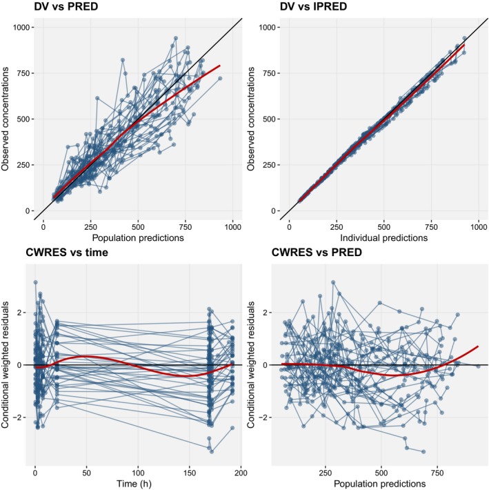
Basic goodness‐of‐fit plots for the final model including covariates. Blue points are observations. Blue lines represent individuals. Red lines are loess smooths through the data. Black lines are lines of identity. CWRES, conditional weighted residuals. DV represents the observations, PRED the predictions, IPRED the individual predictions.

Figure 2.

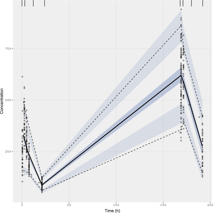
Visual predictive check for the final model including covariates. Black points are original observations. Solid black line is the observed median, by bin. Dashed black lines represent observed 5th and 95th percentiles, by bin. Blue shaded areas represent 90% confidence intervals around simulated 5th, 50^th, and 95th percentiles. Binning at 0, 3, 12, 24, 168, 171, 180, and 192 hours. N = 700 iterations.

nlmixr provides a large number of tuning options and support functions, not discussed here for reasons of space; these are summarized in Supplement S3.

Simulation of new doses and dosing regimen with nlmixr

Simulations of new doses and regimens are easily accomplished by taking advantage of the tight links between nlmixr and RxODE. Simulation designs are constructed by preparing “event tables” defining when doses are given and when observations are made.

ev < - eventTable(amount.units=''mg", time.units=''hours") %>%
add.dosing(dose = 600, nbr.doses = 10, dosing.interval = 24) %>%
add.dosing(dose = 2000, nbr.doses = 5,
start.time = 240,dosing.interval = 48) %>%
add.sampling(0:480);

Here, we have added daily dosing at 600 mg for 10 days, followed by a further 10 days during which the dose is increased to 2000 mg and given every other day. The simulation can be run using the nlmixr fit object using a single command:

sim.2cpt <- simulate(fit.2cpt.ode.saem, events=ev, nSub = 500)

This will generate 500 simulated individuals based on the model and event table. Simulation with uncertainty is possible as well using the nStud argument:

sim.2cpt.unc < - simulate(fit.1cpt.ode.saem,
events=ev, nSub = 500, nStud = 100)

This will generate 50,000 replicates (500x100), including parameter uncertainty as well as between‐subject variability. When parameter uncertainty is included, population parameter estimates are simulated from the multivariate normal distribution and covariance matrix elements from the inverse Wishart distribution. The output is as follows:

print(sim.2cpt.unc)
______________________________ Solved RxODE object _____________________________
-- Parameters (sim.2cpt.unc$params): ----------------------------------------
# A tibble: 50,000 x 11
sim.id eta.v2 eta.v3 eta.ka tka eta.cl tcl eta.q tq tv2 tv3
<int> <dbl> <dbl> <dbl> <dbl> <dbl> <dbl> <dbl> <dbl> <dbl> <dbl>
1 1 0.111 -0.137 -0.0226 0.234 -0.171 -2.97 0.138 -1.22 0.687 2.93
2 2 -0.248 0.151 0.0674 0.234 0.177 -2.97 -0.163 -1.22 0.687 2.93
3 3 0.656 -0.264 -0.457 0.234 -0.584 -2.97 0.213 -1.22 0.687 2.93
4 4 0.380 0.0424 -0.251 0.234 -1.29 -2.97 -0.00105 -1.22 0.687 2.93
5 5 -0.604 0.0256 -0.270 0.234 0.508 -2.97 -0.337 -1.22 0.687 2.93
6 6 -0.0656 0.0241 -0.0171 0.234 0.262 -2.97 0.121 -1.22 0.687 2.93
# ... with 49,994 more rows
-- Initial Conditions (sim.2cpt.unc$inits): ------------------------------
depot center periph
0 0 0
Simulation with uncertainty in:
-- parameters (sim.2cpt.unc$thetaMat for changes)
-- omega matrix (sim.2cpt.unc$omegaList)
-- sigma matrix (sim.2cpt.unc$sigmaList)
-- First part of data (object): --------------------------------------------
# A tibble: 24,050,000 x 4
sim.id time ipred sim
<int> <dbl> <dbl> <dbl>
1 1 0 0 12.2
2 1 1 173. 176.
3 1 2 196. 235.
4 1 3 181. 128.
5 1 4 158. 85.3
6 1 5 137. 102.
# ... with 24,049,994 more rows
----------------------------------------------------------------------------------

Simulation results can be plotted very easily (see Figure  3 for output):

plot(sim.2cpt.unc)

Figure 3.

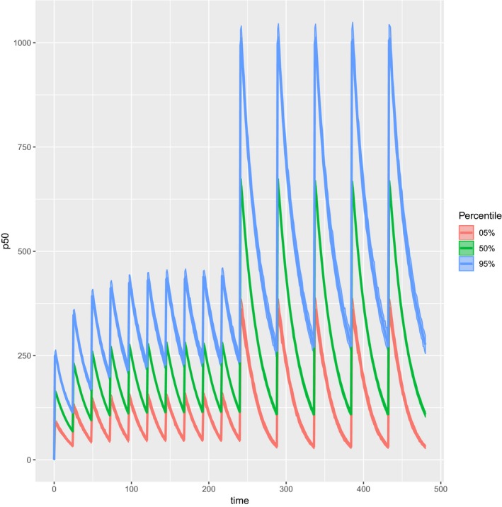
RxODE simulation of final model.

The above example uses the two‐compartment model without covariates. Although covariate effects are not yet directly supported by the nlmixr simulation function, RxODE or other simulation tools may be applied in concert with parameter estimates extracted from the model fit object to generate simulations that include covariate effects across multiple individuals.29

Project‐centric workflow with shinyMixR

The nlmixr package can be accessed directly through the command line in R and additionally through “shinyMixR,” a graphical user interface (GUI) supported by the nlmixr project. The latter enhances the usability and attractiveness of nlmixr, facilitating a dynamic and interactive use in real time for rapid model development. This user‐friendly tool was developed using the R packages “shiny” and “shinydashboards,” and facilitates specifying and controlling an nlmixr project workflow entirely within R. Both command line and graphical interfaces to shinyMixR are supported and in turn support integration with xpose.nlmixr.

The shinyMixR interface provides the possibility to see model run overviews (tabular or interactive graphical trees), compare models, edit models, duplicate models, create new models from templates, run models in separate R sessions, view diagnostic plots (custom or via xpose.nlmixr), and run user‐defined R template scripts and HTML and PDF reporting of tables and plots using the “R3port” package. All this is done within a prespecified folder structure, and the user can always switch between the command line and the interface within the project.

Setting up a project

Project folders can be created with create_proj(). They are populated as follows:

• analysis: in this folder all plots and tables are saved in a structured way to make them accessible to the interface.

• data: data files used by the models in R data format (.rds) or comma‐separated values (CSV).

• models: models available as separate R scripts according the unified user interface in nlmixr.

• scripts: generic analysis scripts made available in the interface, including standard postprocessing scripts.

• shinyMixR: folder used by the interface to store temporary files and results files.

Additions to the overall model structure

The use of shinyMixR requires an addition to the standard nlmixr ini and model blocks. This meta information specifies the dataset, model description, reference model, model importance (overview/tree), and estimation routine with any required control settings within the model itself. The model importance can be used as an indicator if a model is close to final or is important for further steps in model development. This can be useful when filtering the overview and is used to highlight models in the tree overview. When running nlmixr from the command line, the data, estimation routine, and control settings are directly passed to the nlmixr call, whereas the description, reference, and importance are only used in the model overview to provide additional model information.

data = ''theo_sd" # dataset (required)
desc = ''template models" # description of model
ref = '''' # reference model
imp = 1 # importance of model
est = ''saem" # estimation method (required)
control < - saemControl(print = 5) # settings for run (required)
or: control < - list() # minimum setting

When the model is run via shinyMixR, these characteristics are used and stored together with the executed model. The meta information is placed within the model code in a similar way as NONMEM. This ensures that the model, settings, and general information are kept together, improving traceability and reducing sources of error. All input and output are collectively stored. A naming convention is used for shinyMixR models (models are named run[digits]), and file names should be the same as function names.

Fitting models and viewing model output

From the R command line, run the following:

run_shinymixr() # work using shinyMixR GUI

A separate interface window appears (see Figure  4). The available widgets (parameters, overview, goodness of fit, fit plots) provide tools for modeling. The model fit is read in by the interface and custom plots via available postprocessing functionality in the Scripts widget or via xpose.nlmixr can be made.

Figure 4.

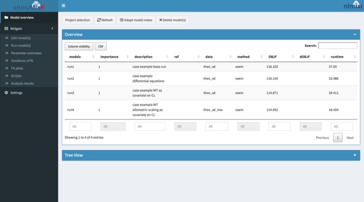
The shinyMixR interface. OBJF is the objective function value; dOBJF is the change in objective function value.

The Analysis results widget can be used to provide standard HTML or PDF reports based on predefined output, such as the parameter table, the goodness of fit, and individual plots via the R3port package.

To use the command line in shinyMixR, run the following:

run_nmx(''run1") # work using shinyMixR command line

Working this way has a number of benefits: runs are executed in a separate R session, preventing crashes in the main session or GUI, and the results are automatically saved to disk, preventing data loss.

Several functions underlying the interface package can be used via the command line (see Supplement S4). As the project folder structure is used, a combination of the shinyMixR interface and the command line interface can be used within the workflow. This enables switching smoothly between the interface and command line within a project.

The model fit can be accessed by reading in the results and plotting them using xpose.nlmixr, functions within shinyMixR, or the user's preferred solution.

fit1 < - readRDS(''shinyMixR/run1.res.rds")
xpdb1 < - xpose_data_nlmixr(fit1)
dv_vs_pred(xpdb1)

Conclusions

nlmixr is an R package for fitting compartmental PK and PK‐PD models described by ODEs. The parameter estimation algorithms implemented in nlmixr currently include relatively mature implementations of nlme, SAEM, and first order, first order with interaction, FOCE, and FOCEi. In addition, adaptive Gaussian quadrature and other estimation routines are planned for integration into the common modeling function or user interface (UI) for formal release in the near future. The package is under intensive development, but is already able to fit complex nonlinear mixed models and has support tools available for graphical diagnostics (xpose.nlmixr), interactive model development (shinyMixR), and reporting (PharmTex13). nlmixr can be used seamlessly as part of complete workflows within R. Coupled with literate programming tools such as knitr and LaTeX, entire analyses can be scripted and reported in a single step (through base R or add‐on packages such as the tidyverse).

Extensive testing has been performed using models of varying complexity against a range of rich and sparse datasets using the nlme, SAEM, and FOCEi algorithms, and both SAEM and FOCEi are very promising. The development version of FOCEi, although less well tested, is capable of producing results comparable to other established tools in terms of parameter estimates, bias, and computational speed. The majority of our experience to date has been with fitting PK models, but nlmixr is fully capable of fitting PD and PK‐PD models as well. Support for models for categorical and other forms of discrete data is planned for the future, and implementation of parallel processing is actively investigated. In addition, automated testing of various nlmixr features and language features has been integrated in Travis CI (Berlin, Germany) and Appveyor (Vancouver, Canada), and selected models are checked before a nlmixr CRAN release.

nlmixr is FOSS, and will remain so; it has no dependencies that are not themselves free and open. Its GPL‐2.0 license requires that directly derivative products share the same “copyleft” licensing provisions, ensuring it will remain free indefinitely. The tool is maintained by a small group of volunteers who oversee nlmixr's development and ensure its continued maintenance and viability. Current members of this team represent large pharmaceutical companies, contract research organizations, and academic institutions. Suggestions and discussions from external users are currently managed by the github issues board and are welcomed.

We believe that nlmixr will continue to evolve into a credible, capable alternative to commercial PK‐PD modeling software, providing a significant unmet need in resource‐poor environments, and that it will stimulate competition and innovation in a niche that lacks open tools. Although we do not believe the tool is sufficiently mature at the current stage to be deployed in a production context in industry, it has already been used for teaching and research in several academic settings,43, 44, 45, 46 and we look forward to its vibrant community of users continuing to grow over time.

Funding

No funding was received for this work.

Conflict of Interest

The authors declared no competing interests for this work.

Supporting information

Supplementary material. True model, intermediate models, and nlmixr options.

Supplementary material. Model data and model script/results.

Example Data Set.

References

- 1. Lalonde, R.L. et al Model‐based drug development. Clin. Pharmacol. Ther. 82, 21–32 (2007). [DOI] [PubMed] [Google Scholar]
- 2. Grasela, T.H. et al Pharmacometrics and the transition to model‐based development. Clin. Pharmacol. Ther. 82, 137–142 (2007). [DOI] [PubMed] [Google Scholar]
- 3. Barrett, J.S. , Fossler, M.J. , Cadieu, K.D. & Gastonguay, M.R. Pharmacometrics: a multidisciplinary field to facilitate critical thinking in drug development and translational research settings. J. Clin. Pharmacol. 48, 632–649 (2008). [DOI] [PubMed] [Google Scholar]
- 4. Mould, D.R. , D'Haens, G. & Upton, R.N. Clinical decision support tools: the evolution of a revolution. Clin. Pharmacol. Ther. 99, 405–418 (2016). [DOI] [PubMed] [Google Scholar]
- 5. Helmlinger, G. et al Drug‐disease modeling in the pharmaceutical industry ‐ where mechanistic systems pharmacology and statistical pharmacometrics meet. Eur. J. Pharm. Sci. 109, S39–S46 (2017). [DOI] [PubMed] [Google Scholar]
- 6. Marshall, S. et al Good practices in model‐informed drug discovery and development: practice, application, and documentation. CPT Pharmacometrics Syst. Pharmacol. 5, 93–122 (2016). [DOI] [PMC free article] [PubMed] [Google Scholar]
- 7. Parekh, A. et al Catalyzing the critical path initiative: FDA's progress in drug development activities. Clin. Pharmacol. Ther. 97, 221–233 (2015). [DOI] [PubMed] [Google Scholar]
- 8. Zvada, S.P. et al Population pharmacokinetics of rifampicin, pyrazinamide and isoniazid in children with tuberculosis: In silico evaluation of currently recommended doses. J. Antimicrob. Chemother. 69, 1339–1349 (2014). [DOI] [PMC free article] [PubMed] [Google Scholar]
- 9. Denti, P. et al Population pharmacokinetics of rifampin in pregnant women with tuberculosis and HIV coinfection in Soweto, South Africa. Antimicrob. Agents Chemother. 60, 1234–1241 (2016). [DOI] [PMC free article] [PubMed] [Google Scholar]
- 10. Svensson, E.M. , Yngman, G. , Denti, P. , McIlleron, H. , Kjellsson, M.C. & Karlsson, M.O. Evidence‐based design of fixed‐dose combinations: principles and application to pediatric anti‐tuberculosis therapy. Clin. Pharmacokinet. 57, 591–599 (2018). [DOI] [PMC free article] [PubMed] [Google Scholar]
- 11. Andrews, K.A. et al Model‐informed drug development for malaria therapeutics. Annu. Rev. Pharmacol. Toxicol. 58, 567–582 (2018). [DOI] [PMC free article] [PubMed] [Google Scholar]
- 12. Mould, D.R. & Upton, R.N. Basic concepts in population modeling, simulation, and model‐based drug development. CPT Pharmacometrics Syst. Pharmacol. 1, e6 (2012). [DOI] [PMC free article] [PubMed] [Google Scholar]
- 13. Mould, D.R. & Upton, R.N. Basic concepts in population modeling, simulation, and model‐based drug development‐part 2: introduction to pharmacokinetic modeling methods. CPT Pharmacometrics Syst. Pharmacol. 2, e38 (2013). [DOI] [PMC free article] [PubMed] [Google Scholar]
- 14. Upton, R.N. & Mould, D.R. Basic concepts in population modeling, simulation, and model‐based drug development: part 3‐introduction to pharmacodynamic modeling methods. CPT Pharmacometrics Syst. Pharmacol. 3, e88 (2014). [DOI] [PMC free article] [PubMed] [Google Scholar]
- 15. Conrado, D.J. , Karlsson, M.O. , Romero, K. , Sarr, C. & Wilkins, J.J. Open innovation: towards sharing of data, models and workflows. Eur. J. Pharm. Sci. 109, S65–S71 (2017). [DOI] [PubMed] [Google Scholar]
- 16. Wilkins, J.J. & Jonsson, E.N . Reproducible pharmacometrics. Abstracts of the Annual Meeting of the Population Approach Group in Europe, Glasgow, Scotland, June 11–14, 2013 < http://www.page-meeting.org/?abstract=2774>.
- 17. Schmidt, H. & Radivojevic, A. Enhancing population pharmacokinetic modeling efficiency and quality using an integrated workflow. J. Pharmacokinet Pharmacodyn. 41, 319–334 (2014). [DOI] [PubMed] [Google Scholar]
- 18. Rasmussen, C.H. et al PharmTeX: a LaTeX‐based open‐source platform for automated reporting workflow. AAPS J 20, 52 (2018). [DOI] [PubMed] [Google Scholar]
- 19. Xie, Y. Dynamic Documents With R and knitr, 2nd edn (Chapman & Hall/CRC, Boca Raton, FL, 2015). [Google Scholar]
- 20. Xie, Y. , Allaire, J.J. & Grolemund, G. R Markdown: The Definitive Guide (Chapman and Hall/CRC, London, UK, 2018) < https://github.com/rstudio/rmarkdown-book>. Accessed June 26, 2018.
- 21. Sahota, T. NMproject: NONMEM Interface in tidyproject. 2018. [Google Scholar]
- 22. Smith, M.K. & Hooker, A. rspeaksnonmem: Read, Modify and Run NONMEM From Within R. 2016. [Google Scholar]
- 23. Lavielle, M. & Chauvin, J. Rsmlx: R Speaks ‘Monolix.’ 2018. [Google Scholar]
- 24. Baker, M. & Penny, D. Is there a reproducibility crisis? Nature 533, 452–454 (2016). [DOI] [PubMed] [Google Scholar]
- 25. Open Science Collaboration. Estimating the reproducibility of psychological science. Science 349, aac4716 (2015). [DOI] [PubMed] [Google Scholar]
- 26. Carpenter, B. et al Stan: a probabilistic programming language. J. Stat. Softw. 76, (2016). 10.18637/jss.v076.i01 [DOI] [PMC free article] [PubMed] [Google Scholar]
- 27. Comets, E. , Lavenu, A. & Lavielle, M. Parameter estimation in nonlinear mixed effect models using saemix, an R implementation of the SAEM algorithm. J. Stat. Softw. 80, 1–42 (2017). [Google Scholar]
- 28. Ihaka, R. & Gentleman, R. R: a language for data analysis and graphics. J. Comput. Graph Stat. 5, 299–314 (1996). [Google Scholar]
- 29. Wang, W. , Hallow, K.M. & James, D.A. A tutorial on RxODE: simulating differential equation pharmacometric models in R. CPT Pharmacometrics Syst. Pharmacol. 5, 3–10 (2016). [DOI] [PMC free article] [PubMed] [Google Scholar]
- 30. Pinheiro, J. & Bates, D. Mixed‐Effects Models in S and S‐PLUS (Springer‐Verlag, New York, 2000). [Google Scholar]
- 31. Delyon, B.Y.B. , Lavielle, M. & Moulines, E. Convergence of a stochastic approximation version of the EM algorithm. Ann. Stat. 27, 94–128 (1999). [Google Scholar]
- 32. Almquist, J. , Leander, J. & Jirstrand, M. Using sensitivity equations for computing gradients of the FOCE and FOCEI approximations to the population likelihood. J. Pharmacokinet Pharmacodyn. 42, 191–209 (2015). [DOI] [PMC free article] [PubMed] [Google Scholar]
- 33. Jonsson, E.N. & Karlsson, M.O. Xpose–an S‐PLUS based population pharmacokinetic/pharmacodynamic model building aid for NONMEM. Comput. Methods Programs Biomed. 58, 51–64 (1999). [DOI] [PubMed] [Google Scholar]
- 34. Hooijmaijers R et al, shinyMixR: Shiny dashboard interface for nlmixr, https://github.com/RichardHooijmaijers/shinyMixR, Accessed 2 July 2019.
- 35. Zhang, X.Y. , Wang, Y.R. , Zhang, Q. & Lu, W. Population pharmacokinetics study of azithromycin oral formulations using NONMEM. Int. J. Clin. Pharmacol. Ther. 48, 662–669 (2010). [DOI] [PubMed] [Google Scholar]
- 36. Meurer, A. et al SymPy: symbolic computing in Python. PeerJ Comput. Sci. 2, e103 (2017). [Google Scholar]
- 37. Ooms, J. , Ripley, B. & Murdoch, D. Building R for windows. CRAN < https://cran.r-project.org/bin/windows/Rtools>. Accessed April 2019.
- 38. Urbanek, S . R for Mac OS X: development tools and libraries. CRAN < https://cran.r-project.org/bin/macosx/tools/>. Accessed April 2019.
- 39. Fidler, M. et al nlmixr: an R package for population PKPD modeling < http://nlmixr.github.io/>. Accessed April 2019.
- 40. Fidler, M. et al nlmixr releases. < http://nlmixr.github.io/>. Accessed April 2019.
- 41. Fidler, M. et al nlmixr github webpage. < http://nlmixr.github.io/>. Accessed April 2019.
- 42. Comets, E. , Brendel, K. & Mentré, F. Computing normalised prediction distribution errors to evaluate nonlinear mixed‐effect models: the npde add‐on package for R. Comput. Methods Programs Biomed. 90, 154–166 (2008). [DOI] [PubMed] [Google Scholar]
- 43. Girard, P. & Mentré, F. A comparison of estimation methods in nonlinear mixed effects models using a blind analysis. Annual Meeting of the Population Approach Group in Europe, Pamplona, Spain, 2005 < https://www.page-meeting.org/default.asp?abstract=834>.
- 44. Erhardt, E. , Jacobs, T. & Gasparini, M. Comparison of pharmacokinetic parameters estimated by the experimental R package “nlmixr” and MONOLIX. Annual Meeting of the Population Approach Group in Europe, Budapest, Hungary, 6 – 9 June, 2017 < https://www.page-meeting.org/default.asp?abstract=7247>.
- 45. Erhardt, E. , Ursino, M. , Jacobs, T. , Biewenga, J. & Gasparini, M. Bayesian knowledge integration for an in vitro–in vivo correlation (IVIVC) model. Annual Meeting of the Population Approach Group in Europe, Montreux, Switzerland, 29 May – 1 June, 2018 < https://www.page-meeting.org/?abstract=8689>.
- 46. Sokolov, V. et al Evaluation of the utility and efficiency of MATLAB and R‐based packages for the development of quantitative systems pharmacology models. Annual Meeting of the Population Approach Group in Europe, Montreux, Switzerland, May 29 – 1 June, 2018. < https://www.page-meeting.org/?abstract=8688>.
Associated Data
This section collects any data citations, data availability statements, or supplementary materials included in this article.
Supplementary Materials