Randomization Tests for Single Case Designs with Rapidly Alternating Conditions: An Analysis of p-Values from Published Experiments

Abstract

Two common barriers to applying statistical tests to single-case experiments are that single-case data often violate the assumptions of parametric tests and that random assignment is inconsistent with the logic of single-case design. However, in the case of randomization tests applied to single-case experiments with rapidly alternating conditions, neither the statistical assumptions nor the logic of the designs are violated. To examine the utility of randomization tests for single-case data, we collected a sample of published articles including alternating treatments or multielement designs with random or semi-random condition sequences. We extracted data from graphs and used randomization tests to estimate the probability of obtaining results at least as extreme as the results in the experiment by chance alone (i.e., p-value). We compared the distribution of p-values from experimental comparisons that did and did not indicate a functional relation based on visual analysis and evaluated agreement between visual and statistical analysis at several levels of α. Results showed different means, shapes, and spreads for the p-value distributions and substantial agreement between visual and statistical analysis when α = .05, with lower agreement when α was adjusted to preserve family-wise error at .05. Questions remain, however, on the appropriate application and interpretation of randomization tests for single-case designs.

To date, visual analysis has been the standard and accepted method for interpreting results of experimental single-case designs (Kratochwill, Levin, Horner, & Swoboda, 2014). Session-by-session data are graphed and inspected with respect to within-condition characteristics (e.g., level, trend, variability) and between-condition characteristics (e.g., immediacy of effect, overlap, consistency; Kratochwill et al., 2010). Visual analysis has a long history in applied behavior analysis and is well aligned with an idiographic approach to answer socially significant research questions (Baer, Wolf, & Risley, 1968; Cooper, Heron, & Heward, 2007; Hagopian et al., 1997; Hopkins, Cole, & Mason, 1998).

However, there may be conditions in which statistical analysis is beneficial. Statistics that quantify the size and direction of an experimental effect can be used to synthesize results across studies, allowing results from single-case work to be included in meta-analyses and evidence-based practice reviews (Shadish, Hedges, Horner, & Odom, 2015). Some have suggested that statistical analyses can also be used to control Type I error when researchers determine whether the effects observed in an experiment are caused by the independent variable (Ferron & Levin, 2014). To aid in making this decision, analysts calculate the probability of obtaining results at least as extreme as the results in the experiment by chance alone (i.e., p-value). Smaller p-values indicate a smaller likelihood that the observed results would occur by chance if the independent variable had no effect on the dependent variable. These p-values can also be used for null hypothesis significance testing when compared to a previously specified level of α (i.e., the tolerated probability of a Type I error, often .05). If the p-value is smaller than α, the null hypothesis that the independent variable had no effect on the dependent variable can be rejected, and results are said to be statistically significant. Because p-values are commonly misinterpreted, it is worth noting that they cannot be used to quantify confidence in the results of a study, nor do they establish the size of the effect of a treatment (Branch, 1999).

Statistical analysis of this kind may be particularly useful when visual analysis is complicated by unstable baselines or variability in data, or when small but reliable differences in behavior are of interest (Kazdin, 1982). Statistical analysis also may be helpful when visual analysts disagree on the interpretation of data. Though some studies have found substantial interrater reliability for decisions made via visual analysis (especially when explicit guidelines are used; e.g., Hagopian et al., 1997; Kahng et al., 2010; Roane, Fisher, Kelley, Mevers, & Bouxsein, 2013), others have found a troubling lack of reliability (e.g., DeProspero & Cohen, 1979; Lieberman, Yoder, Reichow, & Wolery, 2010; Park, Marascuilo, & Gaylord-Ross, 1990). Increasing the objectivity of data analysis is one way to improve reliability, and potentially the validity of conclusions drawn.

It can be difficult to identify a method of statistical analysis suitable for single-case experiments. Commonly used statistical tests in the social sciences, like the paired-sample t test, or the F test in an ANOVA, rely on data assumptions that are rarely met in single-case experiments (Bulté & Onghena, 2008). Namely, these tests assume normally distributed data with equal variance across groups (i.e., homoscedasticity) and that each observation is independent of the others (Howell, 2013). Though these tests are considered robust to violations of the assumptions of normality and homoscedasticity when sample sizes are sufficiently large, results of F and t tests can be biased with small samples or when the assumption of independence is violated (Bulté & Onghena, 2008; Levin, Ferron, & Kratochwill, 2012). If statistical analyses are used to supplement visual analysis, methods are needed that do not rely on as rigorous distributional assumptions. Although nonparametric statistical tests are appropriate alternatives when assumptions for parametric tests are violated, they are less powerful than parametric tests (Siegel, 1957).

One type of nonparametric test, a randomization test, is potentially well-suited for analyzing single-case data (Bulté & Onghena, 2008; Edgington, 1980). Randomization tests are “statistical procedures based on the random assignment of experimental units to treatments to test hypotheses about treatment effects” (Edgington & Onghena, 2007, p. 2), and are used to calculate p-values. They may offer an appealing supplement to visual analysis of single-case experiments for several reasons. First, because these tests create frequency distributions from the obtained data, they do not rely on assumptions about normality and homoscedasticity. However, they retain more power than other tests that do not rely on these assumptions, such as the Kruskal-Wallis test (Adams & Anthony, 1996). Second, randomization tests are flexible in their application. They can be used across different types of data (e.g., continuous, dichotomous, or rank data) and test statistics (e.g., mean difference, median difference). However, they may have lower power when data contain outliers (Branco, Oliveira, Oliveira, & Minder, 2011) or trends (Edgington & Onghena, 2007). Third, at least under some conditions, randomization tests can be used when data are autocorrelated without inflating Type I error (Ferron, Foster-Johnson, & Kromrey, 2003; Levin et al., 2012). Finally, the logic underlying randomization tests is accessible to individuals without extensive training in statistics (Edgington, 1980).

As their name implies, randomization tests require that randomization be incorporated into the experimental design. For single-case experiments, the randomly assigned experimental unit is measurement occasion (Edgington, 1980). That is, to make use of randomization tests, measurement occasions or sessions must be randomly assigned to experimental conditions. In the context of a withdrawal or A-B-A-B design, this could mean randomly determining when in the time series to change conditions (from baseline [A] to intervention [B] or from intervention [B] to baseline [A]). For most single-case researchers, this would represent a departure from current practice where sessions are repeated within conditions until a steady state of responding is observed, at which point a condition change is made. Proponents of randomization tests have argued that incorporating random assignment into single-case research would enhance its credibility, because behavior change following random introduction of an intervention is a strong demonstration of that intervention’s effect (e.g., Kratochwill & Levin, 2010). However, some single-case researchers hold that randomly assigning condition order could decrease, rather than increase, a study’s internal validity and therefore reduce its credibility (e.g., Wolery, 2013). If randomization dictates a change between baseline and intervention before a steady state of responding is established under baseline conditions, variability can obscure any effect the intervention may have had. Or, if a treatment is randomly introduced when a therapeutic trend is evident in baseline, it would be difficult to attribute an improvement following treatment to anything other than the continuation of the baseline trajectory.

Conflicts between the requirements for statistical analysis and the logic of single-case design may explain why randomization tests have not been used more often by single-case researchers. These conflicts are less salient, however, in the context of the alternating treatments design (ATD) and multielement design (MED). In these designs, two or more conditions are rapidly alternated without waiting for a steady state of responding to be established, and each condition is graphed as its own time series (Wolery, Gast, & Ledford, 2018). When visual analysts detect consistent differentiation between conditions, this is interpreted as evidence for a functional relation between the independent and dependent variables. Random assignment of condition order—usually with limits on the maximum number of consecutive observations from the same condition—is sometimes recommended to control for sequence effects in these designs and does not violate the logic of the design (Wolery, 2013). Thus, using randomization tests to evaluate data from ATD and MED experiments represents a unique case where neither the assumptions of the statistical test nor the logic of the single-case design is violated.

The technical properties of randomization tests for time-series data have been established in experiments using simulated Monte Carlo data (e.g., Ferron et al., 2003; Levin et al., 2012). However, randomization tests have rarely been applied to single-case data sets from the behavioral literature. When they have been used to analyze data from applied ATD and MED experiments, they have produced very large (i.e., greater than 0.2) or very small (i.e., less than 0.01) p-values with few values in between (c.f., Bredin-Oja & Fey, 2014; Folino, Ducharme, & Greenwald, 2014; Lloyd, Finley, & Weaver, 2015). If these patterns are typical for applied ATD or MED experiments, the likelihood of Type I errors could meaningfully differ between applied single-case experiments and simulated data sets.

There are also questions about an appropriate α level for significance testing of single-case research. Though .05 is a commonly used threshold for Type I error in the social sciences, that choice is arbitrary and not appropriate for all studies (Nuzzo, 2014). Results of a study by Bartlett, Rapp, and Henrickson (2011) suggested that visual analysis results in a Type I error rate lower than .05. Bartlett et al. graphed randomly generated MED data and asked visual analysts to rate the presence or absence of functional relations for 6,000 graphs. Type I errors were found in fewer than 5% of graphs when conditions included sufficient data (i.e., at least five sessions per condition; Kratochwill et al., 2010) and when guidelines were used for visual analysis. Studies are needed, however, to investigate randomization tests for empirical data sets from ATD and MED experiments and the patterns of p-values they produce.

Purpose

In this article, we give an overview and a hypothetical example of how randomization tests can be applied to ATD and MED experiments and discuss the considerations necessary for doing so. Then, we describe how we identified data sets representative of current practice in single-case research by searching the literature published in peer-reviewed journals for ATD and MED experiments that met current design standards for sufficient data (i.e., five or more sessions per condition; Kratochwill et al., 2010). We describe how we aligned randomization tests with the logic of the experiments. Finally, we examined p-values derived from randomization tests, and their alignment with conclusions drawn by visual analysts. Because the true relationship between dependent and independent variables in a study is unknown, it is not possible to evaluate the accuracy of statistical analyses as applied to published experiments. Rather, we focused on evaluating agreement between visual analysis (as performed by study authors) and statistical analyses. To do so, we restricted our analyses to comparisons that were interpreted by study authors as either demonstrating or not demonstrating a functional relation. We addressed the following research questions:

1. What is the distribution of p-values associated with ATD and MED studies judged via visual analysis to demonstrate the presence of a functional relation?

2. What is the distribution of p-values associated with ATD and MED studies judged via visual analysis to demonstrate the absence of a functional relation?

3. To what extent is there agreement between these visual and statistical analyses about the presence or absence of a functional relation? Does the level of agreement change when different levels of α are selected for the statistical analysis?

Finally, we identify a number of questions that merit future research. We intend for this article to provide a resource for readers interested in statistical analysis of single-case data. We hope to familiarize readers with the logic underlying randomization tests, how this logic relates to the logic of single-case research, and provide an estimate for the correspondence between decisions made with visual and statistical analysis. We also hope to encourage further investigation of when and under what conditions randomization tests may prove useful, and whether certain variants of randomization tests might increase agreement between visual and statistical analysis.

Method

Overview of Randomization Tests

To illustrate how randomization tests work in the context of ATD experiments, consider the hypothetical data set shown in Fig. 1. The graph in the top left panel contains hypothetical data from an ATD. The order of conditions here (T-B-B-T-B-T-B-T-T-B-B-T) is one of 64 possible sequences if each pair of adjacent sessions were randomly assigned to baseline (B) or treatment (T)—such as when a researcher plans to conduct one session of each condition per day and flips a coin to determine which condition is conducted first. The difference between the mean of the treatment condition and the mean of the baseline condition in these hypothetical data is 4.00 responses per minute. The graph in the top right panel depicts the same data and shows the blocks of measurement occasions in which each data point could have been assigned to either condition. The graphs in the bottom panel each represent other possible arrangements of the same data to conditions: T-B-B-T-B-T-T-B-B-T-T-B with a difference of -1.33 and B-T-B-T-B-T-B-T-T-B-T-B with a difference of 0 on the left and right, respectively. Table 1 shows each of the 64 possible mean differences that could have occurred with these data and this randomization scheme, ranked from greatest to least. To calculate the p-value for the hypothetical data in the top left panel of Fig. 1, the number of mean differences greater than or equal to 4.00 (2) is divided by the total number of possible mean differences (64). In this case p = 0.03.

Fig. 1.

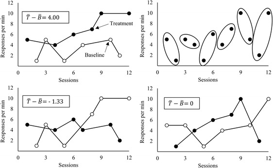
Data from a hypothetical ATD experiment, showing obtained results and associated mean difference (top left), randomization blocks within the experiment (top right) and alternative possible arrangements of data to conditions, with associated mean differences (bottom)

Table 1.

All Possible Mean Differences from Fig. 1 Ranked from Greatest to Least

Rank	$\overline{T}-\overline{B}$	Rank	$\overline{T}-\overline{B}$	Rank	$\overline{T}-\overline{B}$	Rank	$\overline{T}-\overline{B}$	Rank	$\overline{T}-\overline{B}$
1.	4.33	16.	1.33	31.	0.00	46.	-1.33	61.	-3.00
2.	4.00	17.	1.33	32.	0.00	47.	-1.33	62.	-3.33
3.	3.33	18.	1.33	33.	0.00	48.	-1.33	63.	-4.00
4.	3.00	19.	1.33	34.	0.00	49.	-1.33	64.	-4.33
5.	3.00	20.	1.33	35.	0.00	50.	-1.67
6.	2.67	21.	1.00	36.	-0.33	51.	-1.67
7.	2.67	22.	1.00	37.	-0.33	52.	-1.67
8.	2.67	23.	1.00	38.	-0.33	53.	-1.67
9.	2.33	24.	0.67	39.	-0.33	54.	-2.00
10.	2.33	25.	0.67	40.	-0.67	55.	-2.33
11.	2.00	26.	0.33	41.	-0.67	56.	-2.33
12.	1.67	27.	0.33	42.	-1.00	57.	-2.67
13.	1.67	28.	0.33	43.	-1.00	58.	-2.67
14.	1.67	29.	0.33	44.	-1.00	59.	-2.67
15.	1.67	30.	0.00	45.	-1.33	60.	-3.00

This example highlights two important considerations for using randomization tests. One is the direction of the difference being tested. In our earlier example, there are two mean differences that are equal to or greater than the “observed” mean difference (4.00 and 4.33), but there are four mean differences that are equally or more extreme than the observed mean difference (-4.00 -4.33, 4.00 and 4.33). Choosing to calculate ranks based on the value of the difference or the absolute value of the difference is analogous to choosing between one- and two-tailed significance tests. In the context of single-case research, when comparing a treatment to a baseline condition, researchers might predict a directional difference in behavior (e.g., lower rates of problem behavior in a treatment condition relative to baseline). Thus, they may wish to maximize the power of their experiment by only looking for such a difference using a one-tailed test and calculating p-values based on the real value of the mean differences. However, when comparing two treatments, researchers may want to be able to detect a difference favoring either treatment by using a two-tailed test, or by calculating p-values based on the absolute value of the mean differences. This decision should be based on predictions made before data are collected in an experiment. Deciding to use a one-tailed test after observing the difference between conditions increases the probability of Type I errors (Edgington, 1980).

Another consideration is the effect that both the number of data points and the randomization scheme have on test results. All else equal, as the number of data points in an experiment increases, so does the number of possible p-values. More data points mean more possible ways to arrange the data, and therefore more possible mean differences. Likewise, a completely randomized design will produce more possible ways to arrange the data than a randomization scheme in which limits are placed on the number of consecutive sessions from the same condition, or when conditions are randomly ordered within blocks. When the number of possible assignments is small, as in the example above, researchers may calculate each possible difference (this is called a permutation test). When the number of assignments is large (e.g., hundreds of thousands) researchers can calculate values for a randomly selected subset of possible assignments, at the cost of some statistical power (Edgington & Onghena, 2007). In either case, the number of unique possible mean differences affects the number of p-values that can be obtained from the data. In the example above, the total number of possible mean differences is 64, which means the lowest possible p-value in a permutation test is $\frac{1}{64}$ or 0.016.

Because the number of data points can have affect the p-value obtained, the total number of sessions is a decision that is best made before data are collected. Researchers can, whether consciously or unconsciously, bias their results towards smaller p-values if they choose to collect more data points based on observing the graphed data, or if they stop collecting data just as they suspect their results reach significance. In the case of the hypothetical data shown in Fig. 1, early and clear differentiation between conditions is evident. However, such data patterns are not always present in single-case research. When researchers have reason to suspect that differentiation may emerge after participants have been exposed to each condition for several sessions, deciding on a total number of sessions a priori can be difficult. In such cases, a member of the research team may examine graphed data without indication of condition (similar to the top right panel of Fig. 1) as they are collected. This person, a “masked visual analyst,” will be able to offer advice on when to collect more data and when to terminate the experiment without biasing the statistical analysis (Ferron & Levin, 2014).

Eligibility and Inclusion Criteria

We defined inclusion and exclusion criteria for articles (written reports describing the methods and results of one or more original studies), studies (experimental manipulations of independent variables and associated graphical displays of results), and comparisons (evaluations of any pair of conditions in a single study). Articles were eligible for inclusion only if they (a) were published in English in a peer-reviewed journal since 2010; and (b) described and reported the results of an original study on human participants that met inclusion criteria. Studies were eligible for inclusion only if they used an MED or ATD that met current design standards (i.e., experimental manipulations of two or more rapidly alternating conditions where a reversible behavior was measured five or more times in each condition; Kratochwill et al., 2010; Wolery et al., 2018). Further, authors must have alternated conditions according to one of three random or quasi-random methods (e.g., completely randomized, randomized with limits on the maximum number of times a condition could be administered consecutively, or block randomized such that every condition was presented once before any conditions were repeated). Studies in which conditions were alternated using some method other than the three methods described above were excluded. For example, studies were excluded if conditions were alternated in a predetermined counterbalanced order; if two sessions were conducted in a determined order and the third session was randomly assigned; or if conditions were randomized in a block with a limitation on the number of consecutive blocks that could start with the same condition.

Included studies also must have included at least one comparison between conditions that met inclusion criteria. Only pair-wise comparisons that were interpreted by study authors were included in this sample. We considered comparisons to be interpreted if study authors: (a) stated that a functional relation did or did not exist between the independent and dependent variables; (b) used causal language in describing a change in the dependent variable; or (c) used information from a comparison to inform further treatment or analysis (e.g., if a treatment was selected for a “best alone” phase, or if a specific reinforcer from an assessment was used in a treatment). Comparisons were excluded if authors described data patterns (e.g., more responses occurred in Condition A) without including more specific interpretations. Further, interpretations must have been made based on visual analysis, and in accordance with the logic of the alternation design. We excluded comparisons for which interpretations were solely based on quantitative analyses or that were based on comparisons between different phases. Because authors did not always explicitly state their interpretation of a functional relation, or the logic underlying that interpretation, determining whether these inclusion criteria were met involved careful inference. We relied on a coding manual with detailed descriptions of examples and nonexamples to increase the extent to which these inferences were made consistently. This coding manual is presented in Appendix Table 3.

Table 3.

Coding Manual for Determining Inclusion for Articles, Studies, and Comparisons

INCLUSION CODING
ARTICLE LEVEL
Year	Publication year
STUDY LEVEL
Humans	Human participants 0 = no 1 = yes
MED/ATD	Measuring a reversible behavior over two or more rapidly alternating conditions 0 = no 1 = yes
5 Points per	At least two conditions with five or more point each 0 = no 1 = yes
Random	Used a random, semi-random (i.e., random with limits) or block random method of ordering conditions 0 = no 1 = yes Code no if no method of order determination stated, code no if a combination of random methods (e.g., block random with limits on the number of times a given condition could be first)
1 or more included comparison	At least one comparison meets inclusion criteria (determined in the next section of coding) 0 = no 1 = yes
Overall	0 = exclude 1 = include Include if all coded portions are 1 (may stop coding if 0 is coded at any point)
COMPARISON LEVEL
5x5	Both conditions include 5 data points
Visual Analysis	Authors used visual inspection to analyze data 0 = no 1 = yes Assume yes if unstated. If both visual and statistical analyses are used, code yes if visual analysis is the primary method of analysis, or if visual and statistical interpretations are reported in separate sections.
Interpreted	Did the authors come to a conclusion about the presence or absence of a functional relation? 0 = no 1 = yes When present, code first by explicit author interpretation of the presence or absence of a functional relation. Or by explicit author interpretation of a “differentiated” or “undifferentiated” pattern. (Code 1 for both) If none present, consider the following factors: Descriptions or more or less behavior by condition is not enough to code as ‘interpreted’. However, the use of causal language (e.g., “the IV produced” or “the intervention caused” or “reinforcement was effective” or “the treatment failed to change”) can count. Conditional interpretations (“may have an effect” “possibly increased behavior”) should be coded 0. If a group interpretation of results is present (e.g., “the treatment reduced responding in 3 out of four participants”; “for all but one setting, the conditions were not differentiated”) fine to use your own visual analysis skills to figure out which of the graphs/comparisons/participants authors are referring to. FA Interpretation: If a function is identified or ruled out, this is an interpretation of the comparison between the fucntion’s corresponding test condition and the control/play condition. If no functions are identified, (i.e., if FA is undifferentiated) this is an interpretation of all test vs play/control comparisons. Consider “secondary” or “possible” functions to be uninterpreted (code 0). If the FA precedes a treatment, and a reinforcer from the FA is selected for use in the treatment, consider this an interpretation of a functional relation for that reinforcer’s condition. If authors identify an automatic function, no code is implied and you must look for further explanation. If authors justify selection of auto function base on elevated responding in an alone condition, code an interpreted (1) comparison between alone and play. If authors justify selection of auto function based on ruling out all other functions, code comparisons between each test condition and the control condition as interpreted (1). If unclear why, assume not interpreted (0). Test-test comparisons are not interpreted (even if authors report more responding in one vs. another)
Interpretation Consistent with ATD/MED logic	Determination is made by comparing separation by level 0 = no 1 = yes (examples of no: “both treatments worked to reduce problem behavior”—a phase-wise comparison between baseline and intervention ATDs, “treatment A changed problem behavior faster”—AATD-like interpretation of slope, not level)
Overall	0 = exclude 1 = include Include if all coded portions are 1 (may stop coding if 0 is coded at any point)

Finally, studies or comparisons were excluded if the reported randomization scheme did not match the order of conditions depicted in the graph. For example, if authors reported ordering conditions quasi-randomly such that no condition could be repeated more than twice consecutively, but the graph showed three or more consecutive administrations of any condition, that study would be excluded. Studies were also excluded if errors in their graphs made it impossible to extract the necessary data for analysis (e.g., if two conditions were graphed with the same symbol and unlabeled, or if the scale on a y-axis was missing).

Information Sources and Search Strategy

Through ProQuest, we searched the following databases: Published International Literature on Traumatic Stress (PILOTS), ProQuest Criminal Justice, ProQuest Education Journals, ProQuest Family Health, ProQuest Health and Medical Complete, ProQuest Political Science, ProQuest Psychology Journals, ProQuest Social Science Journals, ProQuest Sociology, ProQuest Social Sciences Premium Collection, PsycARTICLES, and PsycINFO. We used the search terms alternating treatment* and multielement or multi-element and restricted results to peer-reviewed journals and articles published after June 2010.

Article Selection and Data Collection Process

We screened the results returned from this search for relevance to the current study. Those that seemed likely to meet inclusion criteria were saved, and their abstracts and graphs were evaluated. Finally, the full text of each article identified in the abstract and graph screening phase was evaluated for adherence to inclusion criteria. For any article selected for inclusion, we coded a series of variables to (a) gather necessary information to construct the research hypothesis (or hypotheses) for each study; (b) determine whether a one- or two-tailed test was appropriate based on that hypothesis; (c) determine the number of possible assignments of sessions to conditions based on the randomization scheme; and (d) note the authors’ interpretation of the data. Then, for all comparisons that met inclusion criteria, we extracted data from the published graphs to perform the randomization tests and calculate p-values.

Coded Variables

At the article level, we collected information on the number of studies that met inclusion criteria and the total number of included comparisons across studies. At the study level, we collected information on the behavior targeted in the study, including how it was measured, and the intended direction (increase or decrease) of behavior change. We noted whether the study was a functional analysis (see “Special considerations,” below). We also recorded the total number of conditions, the number of eligible comparisons, and the randomization scheme used to order conditions (i.e., completely random, random with limits, or block random).

At the comparison level, we coded whether the authors of the article indicated the hypothesized direction of the difference between conditions. We coded this variable first based on any stated hypotheses in the introduction of the article, though these were rarely present. If no hypotheses were stated, we assumed that any comparison between a control, baseline, extinction, typical, or “as usual” condition and an active, treatment, reinforcement, technology-supplemented or novel condition implied a hypothesis that the treatment condition would cause an improvement in behavior relative to the control condition, and we otherwise assumed no directional hypothesis. We also coded whether the authors interpreted the presence or absence of a functional relation. We relied on a coding manual with explicit definitions, examples, and nonexamples to make these decisions consistently, because they frequently involved careful inference (see Appendix Table 4).

Table 4.

Coding Manual for Describing Included Articles, Studies and Comparisons

SAMPLE DESCRIPTION
ARTICLE LEVEL
Author	Enter all authors
Year	Enter publication year
Journal	1—JABA 2—Journal of Special Education Technology 3—American Journal of Speech-Language Pathology 4—Behavior Modification 5—Behaviour Change 6—American Journal of Occupational Therapy 7—Education and Treatment of Children 8—Journal of Autism and Developmental Disorders 9—Journal of Positive Behavior Interventions 10—Analysis of Verbal Behavior 11—Autism 12—Journal of School Psychology 13—Behavior Disorder 14—Developmental Neurorehabilitation 15—Journal of Behavioral Education 16—Disability and Rehabilitation: Assistive Technology 17—Behavioral Interventions 18—Journal of Developmental and Physical Disabilities 19—Research in Autism Spectrum Disorders 20—Journal for the Education of the Gifted 21—Journal of Intellectual Disability Research 22—Learning Disabilities
# of Graphs	Count
STUDY LEVEL
Graph name	Graph identifier—enter name from figure caption
Behavior Target	1 – Decrease 2 – Increase If a purpose is stated by study authors, code based on that. If not, code based on whether the outcome is desirable (e.g., compliance, work accomplished, some measure of learning) or undesirable (e.g., problem behavior, non-engagement). If a traditional FA, the target may be to increase an undesired behavior
DV	1 – count 2 – rate 3 --% of intervals 4—Duration 5--% of trials 6—rating Code by what is presented on the graph’s y-axis
Type	0 – Not FA 1—Yes FA The functional analysis is a method for identifying the effect of environmental variables on the occurrence of behaviors. Code an FA if: a control or play condition is alternated with one or more conditions containing some potentially reinforcing contingency (or potentially evocative condition, if an AB functional analysis or structural analysis). Measured behavior is most likely responses or responses per min, but may also include % of intervals or latency in some cases.
Data Paths	Enter number of data paths on graph, even if only a subset are evaluated (count from graph)
Random	1—block random 2—random with limit 3—completely random Code based on author description of procedures, not based on a guess from the graph. Block random means that all condition are conducted before any are repeated. Authors may use the phrase “block random”, but something like “we conducted each condition each day in a random order” is more likely. Flipping a coin to determine which of two conditions is conducted first is block random if the other condition follows. Drawing lots (without replacement) to determine condition order is also block random. Code 2 if authors indicate a maximum number of times they would repeat a condition consecutively. Code 3 if “random” is indicated, but no limits or information that indicates block randomness is included
Random Method	Describe
# of comparisons	Number of included comparisons
COMPARISON LEVEL
Comparison	Enter name
Directional Hypothesis	1—yes 2—no Code yes if a directional hypothesis explicitly stated in the Introduction. If comparison is obviously comparing a control (or extinction or traditional) condition to an active (or treatment or reinforcement or novel) condition, code yes. If FA code yes. Otherwise code no.
Report Hypothesis	If yes, above, report condition and direction of hypothesis (e.g., “reinforcement higher”; “control lower”)
# of points	Number of points per condition (count from the graph)
Functional relation	0—no 1—yes When present, code first by explicit author interpretation of the presence or absence of a functional relation. Or by explicit author interpretation of a “differentiated” (1) or “undifferentiated” (0) pattern. If none present, consider the following factors: Descriptions or more or less behavior by condition is not enough to code as ‘functional relation’. However, the use of causal language (e.g., “the IV produced” or “the intervention caused” or “reinforcement was effective”) can count. Conditional interpretations (“may have an effect” “possibly increased behavior”) are not interpretations and should have been excluded. Findings of no effect (“no difference between A and B” or “the IV did not change”) code 0. FA Interpretation: If primary behavior function identified, that suggests a functional relation is present for the comparison between that function's condition and Play/Control. If a primary behavior function is ruled out, that function’s condition is undifferentiated with Play/Control, and no functional relation is indicated in that comparison. If behavior function is not identified, (e.g., if FA is described as “inconclusive” or “undifferentiated”) all comparisons between test conditions and Play/Control should be coded 0. If an automatic function is identified, look to the logic of this identification—if an automatic function is identified because all active conditions are ruled out, code a 0 for each comparison between an active condition and Play/Control. If an automatic function is identified because an Alone condition produced higher rates of behavior than the Play/Control condition, code 1 for the Alone vs. Play/Control comparison. Consider “secondary” or “possible” functions to be uninterpreted (should have been excluded). If the FA precedes a treatment, and a reinforcer from the FA is selected for use in the treatment, consider this an interpretation of a functional relation for that reinforcer’s condition. Determinations of functional relations should be drawn from visual analysis of ATD or MED experimental logic. Ignore any conclusions drawn from other logic (e.g., phase-wise logic) if ATD is embedded in another design. If a group interpretation of results (e.g., “the treatment reduced responding in 3 out of four participants”; “for all but one setting, the conditions were not differentiated”) fine to use your own visual analysis skills to figure out which of the graphs/comparisons/participants authors are most likely referring to. If this is impossible to do, default to not interpreted (should have been excluded).

Special Considerations for Functional Analyses

A nontrivial percentage (18%) of the studies we identified reported results of a standard analysis model used to isolate one or more environmental variables that reinforce a targeted behavior (i.e., functional analysis). In a functional analysis, a control or play condition is alternated with one or more conditions designed to test the effects of a potentially relevant reinforcement contingency on the behavior of interest (Hanley, Iwata, & McCord, 2003). The function of a behavior is identified when the level of behavior in a test condition is elevated relative to the control condition. A nonsocial or “automatic” function may be identified if the behavior is elevated in an alone condition relative to other conditions, or if the behavior is elevated and stable in all conditions including the control condition (Hagopian et al., 1997).

We developed a set of guidelines for coding functional analyses in an attempt to align our analysis with the logic of these assessments. First, we associated all comparisons between a test and a control condition in a functional analysis with a directional hypothesis. This is because response differentiation in a functional analysis is considered interpretable if levels of responding in the test condition are higher than, not merely different from, levels in the control condition. If the authors identified or ruled out a specific function, we considered that an interpretation of the comparison between the control condition and the corresponding test condition. If the function was identified, we coded the presence of a functional relation; if the function was ruled out, we coded the absence of a functional relation. If authors identified or ruled out an automatic function, we coded based on the data patterns as described by the authors. If the automatic function was determined because the level of behavior was high and undifferentiated across conditions, we coded this the same as if all tested functions had been ruled out. If the automatic function was interpreted based on elevated responding in an alone or ignore condition relative to other conditions, we coded comparisons between the alone and ignore conditions and those other conditions as having a directional hypothesis and displaying a functional relation.

Interrater Agreement

The first author coded all articles. A second rater (an advanced doctoral student in special education) independently collected data on inclusion/exclusion decisions for studies and comparisons for four randomly selected articles (11% of article sample). Interrater agreement was 92% on study-level inclusion decisions and 94% on comparison-level inclusion decisions. Next, the second rater independently coded all other variables for eight randomly selected articles (22% of article sample). Average agreement was 95% (range, 87%–100%), including 98% agreement on the presence or absence of a functional relation as interpreted by study authors. All disagreements were discussed and resolved.

Data Extraction

We used Plot Digitizer 2.6.8 (Huwaldt, 2015) to extract numerical data from the published graphs. The first author extracted data from all graphs. A second coder extracted data from 42 randomly selected graphs (23% of the sample). We determined that two coders agreed on data extraction for each data point if the extracted x-values (i.e., session numbers) were within 1 and if the extracted y-values were within 1% of the total y-axis. We calculated an exact agreement percentage for each graph by dividing the number of points with agreement by the sum of agreements and disagreements and multiplying by 100. Mean agreement across graphs was 96% (range, 53%–100%). In one graph, an error calibrating the x-axis resulted in many disagreements. This error was corrected for all subsequent graphs, and once the discrepancy from this graph was resolved, mean agreement was 97% (range, 75%–100%). All disagreements were discussed and resolved before data analysis.

Agreement with Author Interpretations

To assess the extent to which errors in author interpretation could have biased our analyses, we randomly selected 20% of included comparisons (32 comparisons that indicated the presence of a functional relation and 23 comparisons that indicated the absence of a functional relation, according to coded author interpretation). We showed the original graphed data to two faculty members and four advanced graduate students in a special education and applied behavior analysis program who regularly conduct single-case research. Each informant independently reviewed the graphs and determined whether each indicated comparison represented the presence or absence of a functional relation based on visual analysis. We calculated agreement between each informant and coded author interpretation, and between each informant and all other informants, by dividing the number of agreements by the number of agreements plus disagreements and multiplying by 100. Independent visual analysts agreed with coded author interpretations about the presence or absence of a functional relation in 90% of cases on average (range, 89%–91%). Independent visual analysts agreed with other visual analysts in 95% of cases on average (range, 92%–98%).

Analytic Strategies

We used the Single-Case Randomization Tests version 1.2 package (Bulté & Onghena, 2017) in R 3.2.4 to analyze the data extracted from included graphs. This package is designed to conduct randomization tests by constructing distributions of possible data arrangements given specific single-case designs and randomization schemes. A thorough description of this package with sample code is available in a tutorial published by the package’s authors (Bulté & Onghena, 2008). We used the pvalue.random function to compare the observed difference between the mean of two conditions to a randomly drawn sample of 10,000 possible differences between the means of the two conditions. Estimates of p-values have been shown to be stable for behavioral data when the distribution contains 10,000 replications (Adams & Anthony, 1996). When the hypothesis was directional, we used the real number difference between means of the condition expected to have a higher level and the condition expected to have a lower level as the test statistic. When the hypothesis was nondirectional we used the absolute value of the difference in means between conditions as the test statistic.

To answer our first two research questions, we calculated means, standard deviations, and ranges for p-values of comparisons judged by authors to (a) demonstrate a functional relation and (b) demonstrate no functional relation, based on visual analysis. To address our third research question, we defined two types of agreements. First, positive agreement was defined as cases in which visual analysis suggested the presence of a functional relation and the p-value was below α (i.e., significant). Second, negative agreement was defined as cases in which visual analysis suggested the absence of a functional relation and the p-value was at or above α (i.e., not significant). We first evaluated agreements when each comparison was considered independent of all others and where α controlled the per comparison rate of Type I error. When studies involved multiple tested comparisons, we also evaluated agreements when α was adjusted using the Holm-Bonferroni method (Holm, 1979) to preserve the family-wise rate of Type I error. For any study with more than one tested comparison, we compared the smallest p-value to $\frac{\alpha }{m}$ where m was the total number of tested comparisons in the study. We compared the next smallest p-value to $\frac{\alpha }{m-1},$ and the next smallest p-value to $\frac{\alpha }{m-2},$ and so on. Any p-value lower than the adjusted α was considered significant. When any comparison had a p-value greater than the adjusted alpha, that p-value and any larger p-values were not significant.

We calculated Cohen’s κ to quantify the agreement between statistical and visual analysis when α was 0.2, 0.1, .05, .01, and .001. Cohen’s κ represents the proportion of agreement after chance agreement is removed (Cohen, 1960). It is calculated with the formula $\mathrm{\kappa }=\frac{p_o-p_c}{1-p_c}$ where p_o is the proportion of cases in which visual and statistical analyses agreed, and p_c is the proportion of cases in which agreement would be expected by chance alone. Here, p_c=(p_VA+ ∗ p_Sig) + (p_VA− ∗ p_Nonsig). That is, chance agreement is estimated as the product of the proportion of cases where visual analysts determined there was a functional relation and the proportion of cases where the p-value was below α, summed with the product of the proportion of cases where visual analysts determined there was no functional relation and the proportion of cases where the p-value was at or above α. Landis and Koch (1977) proposed the following benchmarks for interpreting κ: slight agreement (0.00–0.20), fair agreement (0.21–0.40), moderate agreement (0.41–0.60), substantial agreement (0.61–0.80), and almost perfect agreement (0.81–1.00; p. 165).

Results

Search Results and Sample Selection

Electronic searches returned 1,803 records, 273 of which we identified as likely to meet inclusion criteria and saved for abstract and graph screening. At the graph and abstract screening stage, 106 articles were excluded and 167 articles were saved for full text screening. Of these, we determined that 36 articles met our full inclusion criteria for this analysis. These 36 articles contained 182 eligible studies and 280 eligible comparisons between conditions. The search process is depicted in a flow diagram in Fig. 2.

Fig. 2.

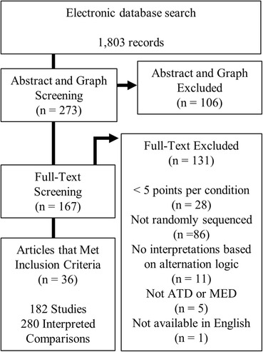
Search process and sample identification

Description of the Sample

The 36 included articles were published in 21 different journals. Ten articles were published in the Journal of Applied Behavior Analysis, five were published in Behavior Modification, and two were published in Education and Treatment of Children and Developmental Neurorehabilitation. The remaining 17 articles were published in 17 different journals. On average, 5.1 eligible studies (range, 1–48) were included per article. Folino et al. (2014) included 48 graphs, presenting results for three dependent variables in four participants four times each day.

Of the 182 included studies, 33 were functional analyses. In 110 studies, the intended direction of change was an increase in behavior, and in 72 studies, the intended direction of change was a decrease in behavior. Across studies, behaviors of interest were measured six ways: percentage of intervals (n = 63), rate (n = 46), count (n = 27), percentage of trials (n = 26), duration (n = 14), and rating (n = 6). Of the 182 studies, 100 used a completely random method of assigning condition order; 33 randomly assigned condition order with a limit on the maximum number of consecutive sessions in any condition; and 49 used a block random method of assigning condition order. Studies contained an average of 2.6 total conditions (range, 2–5) and included an average of 1.5 eligible comparisons (range, 1–4). Included conditions had an average of 7 data points (range, 5–30). Of the 280 included comparisons, the majority (238) had a stated or implied directional hypothesis. For 162 comparisons, authors determined that the data depicted a functional relation between the independent and dependent variables; for 118 comparisons, authors found no functional relation.

P-Value Distributions

The distributions of p-values for comparisons that did and did not indicate functional relations based on visual analysis are depicted in the strip chart in Fig. 3. The vast majority of the p-values from comparisons in which authors detected a functional relation were below .05 and are arranged in a right-skewed distribution. The p-values from comparisons in which authors did not detect a functional relation are arranged in a nearly uniform distribution covering the entire range of possible values. Observed p-values were lower on average (M = 0.035) for comparisons indicating functional relations relative to comparisons that did not indicate a functional relation (M = 0.473). P-values associated with comparisons that did not indicate functional relations were more widely dispersed (SD = 0.347) than those associated with comparisons that did indicate functional relations (SD = 0.09). However, ranges of p-values were similar between comparisons that did (range, <0.0001–0.858) and did not (range, 0.004–0.999) indicate functional relations.

Fig. 3.

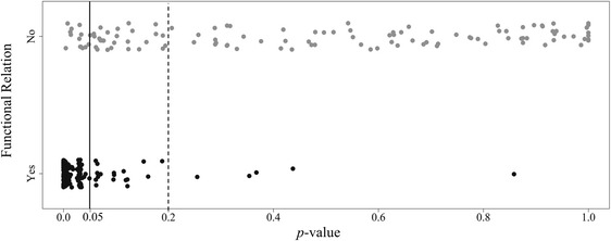
A plot of the distribution of p-values associated with comparisons authors interpreted as demonstrating (black points) and not demonstrating (gray points) functional relations. The solid line marks .05, and the dashed line marks .2

Agreement between Visual and Statistical Analyses with per Comparison α

As displayed in Fig. 4, when α was used to control per comparison Type I error rates, agreement between statistical and visual analyses varied across criterion α values but was highest (and substantial) when α = .05 (κ = 0.746). Agreement was fair when α = .001 (κ = 0.217); moderate when α = .01 (κ = 0.492); and substantial when α = .1 (κ = 0.709) and α = .2 (κ = 0.657; Landis & Koch, 1977). The relationship between α levels and the degree of agreement between visual and statistical analysis can be further inspected in Fig. 3. Gray data points represent comparisons that did not demonstrate a functional relation per author interpretation. When α = .05 (represented by the solid vertical line) and controls per comparison error, gray data points to the left of the solid line represent cases of disagreement between visual and statistical analyses (i.e., no functional relation based on visual analysis and p < .05) and gray data points to the right of the solid line represent cases of negative agreement (i.e., no functional relation based on visual analysis and p > .05). Black data points represent comparisons that did represent a functional relation per author interpretation. When per comparison α = .05, black data points to the left of the solid line indicate cases of positive agreement between visual and statistical analyses (i.e., functional relation based on visual analysis and p < .05) and black data points to the right of the solid line indicate cases of disagreement (i.e., functional relation based on visual analysis and p > .05).

Fig. 4.

A bar graph of Cohen’s κ indicating agreement between visual and statistical analyses, across different α values where family-wise error (white bars) and per comparison error (gray bars) are considered. Error bars represent 95% confidence intervals

To understand how the criterion α alters κ, consider moving the vertical line. If the per comparison α were increased (i.e., if the vertical line shifted to the right) the number of cases representing positive agreements would increase in the black distribution, but the number of cases representing negative agreement would decrease in the gray distribution. For example, if we increase α from .05 to .2, at the dashed vertical line, there would be 17 more cases of agreement in the black distribution (i.e., 17 more black data points to the left of the dashed line), but 27 fewer cases of agreement in the gray distribution (i.e., 27 more gray data points to the right of the dashed line). Thus, overall there would be 10 fewer agreements if α increased from .05 to .2, which accounts for the decline in κ. If α decreased, the number of cases representing positive agreements would decrease in the black distribution, but the number of cases representing negative agreement would increase in the gray distribution.

Because many p-values associated with a functional relation were densely clustered below .05, decreasing α means that many more agreements were lost in the black distribution than were gained in the gray distribution. Overall, there were 40 fewer agreements when α was reduced from .05 to .01, and another 47 fewer agreements when α was reduced from .01 to .001. This accounts for the steeper decline in κ when α decreased, relative to when α increased, as shown in Fig. 4. Frequencies of agreements and disagreements in both distributions by level of per comparison α are presented on the left side of Table 2.

Table 2.

Agreement Matrix Across Per Comparison and Family-wise Alpha Levels

Per Comparison α		Visual Analysis		Family-wise α		Visual Analysis
		Functional Relation	No Functional Relation			Functional Relation	No Functional Relation
.2	Significant Not Significant	157 5	40 78	.2	Significant Not Significant	155 7	32 86
.1	Significant Not Significant	150 12	27 91	.1	Significant Not Significant	140 22	17 101
.05	Significant Not Significant	140 22	13 105	.05	Significant Not Significant	105 57	5 113
.01	Significant Not Significant	89 73	2 116	.01	Significant Not Significant	83 79	2 116
.001	Significant Not Significant	40 122	0 118	.001	Significant Not Significant	39 123	0 118

Note. Bolded numbers indicate cases of agreement

Agreement between Visual and Statistical Analyses with Family-Wise α

As displayed in Fig. 4, when we adjusted α to control family-wise error rates when studies included multiple comparisons, agreement at α = .05 decreased to κ = 0.572, reflecting only moderate agreement. For other values of α, however, similar levels of agreement were identified when we used family-wise and per comparison α. Agreement was still fair when the adjusted α = .001 (κ = 0.211); moderate when α = .01 (κ = 0.455); and substantial when α = .1 and α = .2 (κ = 0.716 and κ = 0.706, respectively). Frequencies of agreements and disagreements in both distributions by level of family-wise α are presented on the right side of Table 2.

As above, the reasons for this change in agreement can be seen in Fig. 3. Many p-values associated with a functional relation were at or near .03; these cases can be seen arranged in a clustered column to the left of .05 in the black distribution in Fig. 3. If a study involved two comparisons (e.g., between baseline and each of two treatments) a p-value of .03 would be significant at an α of .05 but not significant when the α is adjusted to preserve family-wise error rate (.03 >$\frac{.05}{2}$). This clustering of values may be related to our decision to include only studies with sufficient data to meet current design standards (i.e., five or more sessions per condition; Kratochwill Levin et al., 2010). As noted above, the number of data points and the randomization scheme determine the number of possible arrangements of the data, and therefore affect the range of possible p-values. If conditions are randomized in a block, and five sessions are conducted per condition, the number of possible arrangements of the data (and therefore the number of possible differences between means) is 2⁵, or 32. Thus, the largest positive difference between conditions would likely produce a p-value of $\frac{1}{32}$ or .031. Of the 39 p-values associated with a functional relation that were between .025 and .04, 26 are from block randomized comparisons between two conditions with five data points each. Twenty-three of these were cases with multiple comparisons that changed from agreements to disagreements at α = .05 when α was adjusted to preserve family-wise error rate.

Discussion

In this study, we identified a sample of published ATD and MED studies that used random or quasi-random assignment to determine the order of experimental conditions. We extracted data from these studies and used randomization tests to calculate p-values for the comparisons between conditions in these experiments. We compared the distribution of p-values for comparisons identified as representing a functional relation based on visual analysis, and for those identified as representing no functional relation. P-values from comparisons that did and did not suggest functional relations based on visual analysis seemed to form different distributions with different means, shapes and spreads. Finally, we calculated Cohen’s κ to quantify the level of agreement between visual and statistical analyses based on five different values for α. When we considered only per comparison error, we found substantial agreement between visual and statistical analyses when α was set at .05, but declining levels of agreement when α was greater than or less than .05. When we adjusted α to control family-wise error rate in studies with multiple comparisons, we found lower agreement between visual and statistical analyses at α = .05, relative to the agreement when our tests of significance did not consider family-wise error rate. Levels of agreement at other family-wise α levels were similar to their per comparison counterparts. Of course, agreement is not the same as accuracy and an analysis of agreement should not be interpreted as an evaluation of the validity of using .05 as α or of the importance of considering family-wise error.

One way to evaluate the validity of a statistical test is to determine whether the rate of false positives is held at or below α (i.e., if α is .05, whether statistically significant results occur less than 5% of the time when the null hypothesis is true; Edgington & Onghena, 2007). In this case, if we assume visual analysts correctly judged the absence of a functional relation, we may look at the 118 comparisons where they did so, and evaluate the proportion of comparisons that were below each evaluated α. When α controls per comparison error, in those 118 comparisons, 33.8% of p-values were below .2, 24.5% were below .1, 11.0% were below .05, and 1.6% were below .01. No p-values from comparisons judged not to represent a functional relation were below .001. This means the incidence of false positives was 1.6 to 2.5 times higher than expected for every α except .001 when each comparison is evaluated independently. As might be expected, when α is adjusted to control family-wise error rate, the rate of false positives was lower. Only 27% of p-values judged not to represent a functional relation were significant at a family-wise α of .2, 14% at .1, and 4% at .05 (the number of false positives at α = .01 and α = .001 do not change when α is adjusted to preserve family-wise error rate). It should be noted that this subset of comparisons is small and may not be representative of cases where the null hypothesis is true. We only included comparisons that authors explicitly interpreted, which was not every possible comparison in every included study. It is possible that authors were less likely to explicitly identify the absence of a functional relation than they were to identify the presence of a functional relation.

On the other hand, it may be the case that statistical significance correctly identifies a true experimental effect at some value for α. If we assume statistical significance at a per comparison α of .05 is the gold standard, for example, visual analysis misses 8% (13 of 153) of significant comparisons. Visual analysis misses 15% (27 of 177) of significant comparisons when per comparison α is .1, and 2% (2 of 91) of significant comparisons when per comparison α is .01. The uniform distribution of p-values for comparisons judged by visual analysts to not represent a functional relation (Fig. 3, top) may suggest that visual analysis is biased in favor of finding no effect. There is no point along this distribution where p-values become less common than would be predicted by chance; they are approximately uniformly likely across the range of possible p-values. Contrast this with the distribution of p-values associated with a functional relation (Fig. 3, bottom), which is skewed to the right, with many more p-values than would be expected by chance alone falling below .05, and p-values becoming markedly less common above .05. We would expect to see a reciprocal thinning of the frequency of p-values below .05 for comparisons judged to not represent a functional relation, but that is not evident in this data set. Although this could mean visual analysis is too conservative in some cases, a more likely explanation is that visual analysts are attending to features of the data that are not captured in the statistical analysis (e.g., data stability, consistency of difference between conditions, effects observed in other conditions or for other participants).

Limitations

Our results should be interpreted in light of three main limitations. First, given our search and screening procedures this study should not be interpreted as containing an exhaustive set of all ATD and MED experiments. Our search would only have identified articles indexed in the databases we searched, and articles where the authors used the terms “multielement” and “alternating treatment/s” to describe their experiments. Further, we did not assess interrater agreement on inclusion and exclusion decisions related to articles. We did, however, assess interrater agreement on inclusion and exclusion decisions at the study and comparison level for 11% of included articles, and agreement was high (92% and 94%, respectively). The decisions necessary to include or exclude studies and comparisons were much more complex than the decisions necessary to include or exclude articles. Study and comparison inclusion decisions involved decisions about hypotheses, interpretations of effect, and experimental logic. Article inclusion was determined by publication year, and whether the article contained an eligible study. Because we have an estimate of reliability on the most complicated inclusion decisions, we suspect but cannot confirm that agreement on article inclusion decisions would have been similarly high had we assessed it. However, we cannot rule out the possibility that articles were inappropriately excluded from our sample in the screening process.

Second, we relied on author interpretations of functional relations based on visual analysis; we did not ask independent visual analysts to reinterpret the graphed data for all included comparisons. Any errors in visual analysis by authors may have skewed our results. However, we did observe high agreement (90%) between independent visual analysists and coded author decisions on the subset of studies for which we assessed agreement. Finally, in our analyses, we only used the absolute value of the difference between condition means as the test statistic when two novel treatments were compared and authors presented no hypothesis about which treatment was superior. We did not use the absolute value of the differences between condition means to detect countertherapeutic effects of a treatment relative to baseline or no treatment conditions. We made this decision because baseline and no treatment conditions in single-case research are usually constructed to isolate the independent variable, not to represent typical practice (Wolery, 2013). It is important to note that as a consequence of this decision the majority of the p-values we calculated were analogous to one-tailed tests. This could bias our results towards smaller p-values compared to an analysis that made more frequent use of the absolute value of the difference between condition means (analogous to two-tailed tests).

Future Directions

It is unlikely that either visual or statistical analysis using any α were correct about the true relationship between independent and dependent variables in all cases presented in this study. Visual analysts may have had varying levels of skill, and peer review of their conclusions may have been done with varying levels of quality. Data display features, such as the number of data paths on a graph or the variability of data, may have made visual analysis more difficult or prone to error in some cases than others (Bartlett et al., 2011; Matyas & Greenwood, 1990). On the other hand, outliers, trends, or floor/ceiling effects may have skewed statistical analyses in some cases. Though we focused on quantifying agreement in this study, future research on the factors that contribute to disagreement is warranted. For example, in this study we used differences between condition means, but other measures of central tendency (e.g., median, trimmed mean) may be more appropriate for analyzing some single-case experiments and may bring statistical analyses more in line with visual analysis. Moreover, measures that are influenced by the consistency of difference between conditions (e.g., overlap metrics, binomial sign tests) may be better aligned with how visual analysists make decisions for designs involving rapidly alternating conditions. Future work comparing levels of agreement between visual analysis and randomization tests conducted with different test statistics are needed to evaluate the utility of these tests. As an alternative, test statistics may need to be selected a priori for individual single-case experiments based on what features of the data are predicted to change between or among conditions.

In addition, future work will be necessary to consider whether the requirements for sufficiently powered randomization tests are always compatible with the logic of single-case experiments, especially when considering family-wise error rate. In this study, we chose to focus on analyzing ATD and MED experiments with randomization tests, because there is substantial alignment between the requirements of the tests and the logic of the designs. However, this alignment was challenged when we altered α to preserve family-wise error rate at .05. Many cases that represented positive agreement between visual and statistical analysis when .05 was the per comparison α changed to cases of disagreement when we corrected for multiple comparisons. In many of these cases, comparisons were between conditions with few data points that were block randomized, which limited the number of possible arrangements of the data. It is interesting to note that 23 cases (or 66% of the 35 cases that changed from agreement to disagreement on considering family-wise error rate) were perfectly differentiated comparisons between five-session conditions randomized in blocks. In one case, drawn from a functional analysis of nonengaged behavior conducted by Camacho, Anderson, Moore, and Furlonger (2014), problem behavior was observed for 100% of the time in each of five sessions in a test condition and 0% of the time in each of five sessions in a control condition. The p-value associated with this comparison was .031; significant at .05, but not significant when compared to $\frac{.05}{2}$ to account for other tested comparisons from the same functional analysis.

In the context of group design experiments, where the problems of multiple comparisons in a single study are well-documented, increasing sample size to preserve power when multiple comparisons will be conducted is frequently recommended (c.f. Levin, 1975). In this case, researchers might be advised to collect more data or alter the randomization scheme. We suspect that for most single-case researchers, a recommendation to collect more data after observing five pairs of test and control data points at opposite ends of the y-axis would seem unnecessary.

This concern is especially relevant when considering the functional analysis, where two or more test conditions are often compared to a control condition in the same study (Hanley et al., 2003). If two test conditions are conducted and block randomized (as in the example above), even consistent differentiation between fewer than six test and control sessions will not produce a significant p-value when family-wise error rate is controlled at .05. If four block randomized test conditions are conducted, at least seven of each test and control conditions must be consistently differentiated before we would expect a significant p-value. Under current ATD and MED standards, five sessions of each condition would be sufficient to establish a functional relation in either case (Wolery et al., 2018). Work towards developing consensus in the field about when and how to correct α to preserve family-wise error rate is needed, as is empirical work exploring the consequences of considering only the per comparison error rate in ATD and MED studies. Investigating these issues may help single-case researchers evaluate the benefits of statistical testing, and whether the requirements for their use align with single-case logic.

Conclusion

Unlike other statistical tests applied to single-case experiments, applying nonparametric randomization tests to MED and ATD experiments violates neither the assumptions necessary for a statistical analysis nor the logic of the single-case design. Although studies using hypothetical data suggest these applications may be useful, how these tests perform on applied single-case data sets is largely unknown. In this study, we found substantial alignment between decisions made with visual and statistical methods in a sample of published single-case research when comparisons are considered independently. However, many questions remain with respect to how these tests should be applied and interpreted in the context of single-case research.

Compliance with Ethical Standards

Conflict of Interest

The authors declare that they have no conflict of interest.

References

References marked with an asterisk (*) contain data analyzed in this study.
- Adams DC, Anthony CD. Using randomization techniques to analyse behavioural data. Animal Behaviour. 1996;51:733–738. [Google Scholar]
- Baer DM, Wolf MM, Risley TR. Some current dimensions of applied behavior analysis. Journal of Applied Behavior Analysis. 1968;1:91–97. doi: 10.1901/jaba.1968.1-91. [DOI] [PMC free article] [PubMed] [Google Scholar]
- Bartlett SM, Rapp JT, Henrickson ML. Detecting false positives in multielement designs: implications for brief assessments. Behavior Modification. 2011;35:531–552. doi: 10.1177/0145445511415396. [DOI] [PubMed] [Google Scholar]
- *Betz, A. M., Fisher, W. W., Roane, H. S., Mintz, J. C., & Owen, T. M. (2013). A component analysis of schedule thinning during functional communication training. Journal of Applied Behavior Analysis, 46, 219–241. 10.1002/jaba.23. [DOI] [PubMed]
- Branch MN. Statistical inference in behavior analysis: some things significance testing does and does not do. Behavior Analyst. 1999;22(2):87–92. doi: 10.1007/BF03391984. [DOI] [PMC free article] [PubMed] [Google Scholar]
- Branco F, Oliveira TA, Oliveira A, Minder CE. The impact of outliers on the power of the randomization test for two independent groups. American Institute of Physics Conference Proceedings. 2011;1389:1545–1548. [Google Scholar]
- *Bredin-Oja, S., & Fey, M. E. (2014). Children’s responses to telegraphic and grammatically complete prompts to imitate. American Journal of Speech-Language Pathology, 23(1), 15–26. 10.1044/1058-0360(2013/12-0155). [DOI] [PubMed]
- *Bryant, B. R., Kim, M. K., Ok, M. W., Kang, E. Y., Bryant, D. P., Lang, R., & Son, S. H. (2015). A comparison of the effects of reading interventions on engagement and performance for fourth-grade students with learning disabilities. Behavior Modification, 39(1), 167–190. 10.1177/0145445514561316. [DOI] [PubMed]
- Bulté I, Onghena P. An R package for single-case randomization tests. Behavior Research Methods. 2008;40:467–478. doi: 10.3758/brm.40.2.467. [DOI] [PubMed] [Google Scholar]
- Bulté, I., & Onghena, P. (2017). SCRT: single-case randomization tests. R package version. 1.2. Retrieved from https://CRAN.R-project.org/package=SCRT [DOI] [PubMed]
- *Camacho, R., Anderson, A., Moore, D. W., & Furlonger, B. (2014). Conducting a function-based intervention in a school setting to reduce inappropriate behaviour of a child with autism. Behaviour Change, 31(1), 65–77. 10.1017/bec.2013.33.
- *Casella, S. E., Wilder, D. A., Neidert, P., Rey, C., Compton, M., & Chong, I. (2010). The effects of response effort on safe performance by therapists at an autism treatment facility. Journal of Applied Behavior Analysis, 43, 729–734. 10.1901/jaba.2010.43-729. [DOI] [PMC free article] [PubMed]
- *Chung, Y., & Cannella-Malone, H. (2010). The effects of presession manipulations on automatically maintained challenging behavior and task responding. Behavior Modification, 34(6), 479–502. 10.1177/0145445510378380. [DOI] [PubMed]
- Cohen J. A coefficient of agreement for nominal scales. Education & Psychological Measurement. 1960;20(1):37–46. [Google Scholar]
- Cooper JO, Heron TE, Heward WL. Applied behavior analysis. 2. Upper Saddle River, NJ: Pearson; 2007. [Google Scholar]
- *Crowe, T. K., Perea-Burns, S., Sedillo, J. S., Hendrix, I. C., Winkle, M., & Deitz, J. (2014). Effects of partnerships between people with mobility challenges and service dogs. American Journal of Occupational Therapy, 68(2), 194–202. 10.5014/ajot.2014.009324. [DOI] [PubMed]
- *Crowley-Koch, B. J., Houten, R., & Lim, E. (2011). Effects of pedestrian prompts on motorist yielding at crosswalks. Journal of Applied Behavior Analysis, 44, 121–126. 10.1901/jaba.2011.44-121. [DOI] [PMC free article] [PubMed]
- *Davis, T. N., Durand, S., Fuentes, L., Dacus, S., & Blenden, K. (2014). The effects of a school-based functional analysis on subsequent classroom behavior. Education & Treatment of Children, 37(1), 95–110. 10.1353/etc.2014.0009.
- DeProspero A, Cohen S. Inconsistent visual analyses of intrasubject data. Journal of Applied Behavior Analysis. 1979;12:573–579. doi: 10.1901/jaba.1979.12-573. [DOI] [PMC free article] [PubMed] [Google Scholar]
- *Devlin, S., Healy, O., Leader, G., & Hughes, B. M. (2011). Comparison of behavioral intervention and sensory-integration therapy in the treatment of challenging behavior. Journal of Autism & Developmental Disorders, 41, 1303–1320. 10.1007/s10803-010-1149-x. [DOI] [PubMed]
- Edgington ES. Validity of randomization tests for one-subject experiments. Journal of Educational Statistics. 1980;5(3):235–251. [Google Scholar]
- Edgington E, Onghena P. Randomization tests. Boca Raton, FL: CRC Press; 2007. [Google Scholar]
- *Faul, A., Stepensky, K., & Simonsen, B. (2012). The effects of prompting appropriate behavior on the off-task behavior of two middle school students. Journal of Positive Behavior Interventions, 14(1), 47–55. 10.1177/1098300711410702.
- *Ferreri, S. J., & Plavnick, J. B. (2011). A functional analysis of gestural behaviors emitted by young children with severe developmental disabilities. Analysis of Verbal Behavior, 27, 185–190. 10.1007/BF03393101. [DOI] [PMC free article] [PubMed]
- Ferron J, Foster-Johnson L, Kromrey JD. The functioning of single-case randomization tests with and without random assignment. Journal of Experimental Education. 2003;71(3):267–288. [Google Scholar]
- Ferron JM, Levin JR. Single-case permutation and randomization statistical tests: present status, promising new developments. In: Kratochwill TR, Levin JR, editors. Single-case intervention research: methodological and statistical advances. Washington, DC: American Psychological Association; 2014. pp. 153–183. [Google Scholar]
- *Finnigan, E., & Starr, E. (2010). Increasing social responsiveness in a child with autism: a comparison of music and non-music interventions. Autism, 14, 321–348. 10.1177/1362361309357747. [DOI] [PubMed]
- *Folino, A., Ducharme, J. M., & Greenwald, N. (2014). Temporal effects of antecedent exercise on students' disruptive behaviors: an exploratory study. Journal of School Psychology, 52, 447–462. 10.1016/j.jsp.2014.07.002. [DOI] [PubMed]
- Hagopian LP, Fisher WW, Thompson RH, Owen-DeSchryver J, Iwata BA, Wacker DP. Toward the development of structured criteria for interpretation of functional analysis data. Journal of Applied Behavior Analysis. 1997;30:313–326. doi: 10.1901/jaba.1997.30-313. [DOI] [PMC free article] [PubMed] [Google Scholar]
- *Hammond, J. L., Iwata, B. A., Rooker, G. W., Fritz, J. N., & Bloom, S. E. (2013). Effects of fixed versus random condition sequencing during multielement functional analyses. Journal of Applied Behavior Analysis, 46, 22–30. 10.1002/jaba.7. [DOI] [PubMed]
- Hanley GP, Iwata BA, McCord BE. Functional analysis of problem behavior: a review. Journal of Applied Behavior Analysis. 2003;36:147–185. doi: 10.1901/jaba.2003.36-147. [DOI] [PMC free article] [PubMed] [Google Scholar]
- *Haydon, T., Hawkins, R., Denune, H., Kimener, L., McCoy, D., & Basham, J. (2012). A comparison of iPads and worksheets on math skills of high school students with emotional disturbance. Behavioral Disorders, 37, 232–243.
- Holm S. A simple sequentially rejective multiple test procedure. Scandinavian Journal of Statistics. 1979;6(2):65–70. [Google Scholar]
- Hopkins BL, Cole BL, Mason TL. A critique of the usefulness of inferential statistics in applied behavior analysis. Behavior Analyst. 1998;21:125–137. doi: 10.1007/BF03392787. [DOI] [PMC free article] [PubMed] [Google Scholar]
- Howell DC. Statistical methods for psychology. 8. Belmont, CA: Wadsworth; 2013. [Google Scholar]
- Huwaldt, J. A. (2015). Plot Digitizer 2.6.8 [computer software]. Retrieved from https://sourceforge.net/projects/plotdigitizer/.
- Kahng SW, Chung KM, Gutshall K, Pitts SC, Kao J, Girolami K. Consistent visual analyses of intrasubject data. Journal of Applied Behavior Analysis. 2010;43:35–45. doi: 10.1901/jaba.2010.43-35. [DOI] [PMC free article] [PubMed] [Google Scholar]
- *Kang, S., O'Reilly, M. F., Fragale, C. L., Aguilar, J. M., Rispoli, M., & Lang, R. (2011). Evaluation of the rate of problem behavior maintained by different reinforcers across preference assessments. Journal of Applied Behavior Analysis, 44, 835–846. 10.1901/jaba.2011.44-835. [DOI] [PMC free article] [PubMed]
- Kazdin AE. Single-case research designs: methods for clinical and applied settings. New York, NY: Oxford University Press; 1982. [Google Scholar]
- *Kenzer, A. L., Bishop, M. R., Wilke, A. E., & Tarbox, J. R. (2013). Including unfamiliar stimuli in preference assessments for young children with autism. Journal of Applied Behavior Analysis, 46(3), 689–694. 10.1002/jaba.56. [DOI] [PubMed]
- Kratochwill, T. R., Hitchcock, J., Horner, R. H., Levin, J. R., Odom, S. L., Rindskopf, D. M., & Shadish, W. R. (2010). Single-case designs technical documentation. Retrieved from http://files.eric.ed.gov/fulltext/ED510743.pdf.
- Kratochwill TR, Levin JR. Enhancing the scientific credibility of single-case intervention research: randomization to the rescue. Psychological Methods. 2010;15:124–144. doi: 10.1037/a0017736. [DOI] [PubMed] [Google Scholar]
- Kratochwill TR, Levin JR, Horner RH, Swoboda CM. Visual analysis of single-case intervention research: conceptual and methodological issues. In: Kratochwill TR, Levin JR, editors. Single-case intervention research: methodological and statistical advances. Washington, DC: American Psychological Association; 2014. pp. 91–125. [Google Scholar]
- Landis JR, Koch GG. The measurement of observer agreement for categorical data. Biometrics. 1977;33(1):159–174. [PubMed] [Google Scholar]
- Levin JR. Determining sample size for planned and post hoc analysis of variance comparisons. Journal of Educational Measurement. 1975;12(2):99–108. [Google Scholar]
- Lieberman RG, Yoder PJ, Reichow B, Wolery M. Visual analysis of multiple baseline across participants graphs when change is delayed. School Psychology Quarterly. 2010;25:28–44. [Google Scholar]
- Lee A, Lang R, Davenport K, Moore M, Rispoli M, van der Meer L, Chung C. Comparison of therapist implemented and iPad-assisted interventions for children with autism. Developmental Neurorehabilitation. 2015;18(2):97–103. doi: 10.3109/17518423.2013.830231. [DOI] [PubMed] [Google Scholar]
- *Legray, M. W., Dufrene, B. A., Sterling-Turner, H., Olmi, D. J., & Bellone, K. (2010). A comparison of function-based differential reinforcement interventions for children engaging in disruptive classroom behavior. Journal of Behavioral Education, 19(3), 185–204. 10.1007/s10864-010-9109-2.
- *Lemoncello, R., Sohlberg, M. M., Fickas, S., Albin, R., & Harn, B. E. (2011). Phase I evaluation of the television assisted prompting system to increase completion of home exercises among stroke survivors. Disability & Rehabilitation: Assistive Technology, 6, 440–452. 10.3109/17483107.2010.542571. [DOI] [PubMed]
- *Lequia, J., Machalicek, W., & Lyons, G. (2013). Parent education intervention results in decreased challenging behavior and improved task engagement for students with disabilities during academic tasks. Behavioral Interventions, 28, 322–343. 10.1002/bin.1369.
- Levin JR, Ferron JM, Kratochwill TR. Nonparametric statistical tests for single-case systematic and randomized ABAB. .. AB and alternating treatment intervention designs: new developments, new directions. Journal of School Psychology. 2012;50:599–624. doi: 10.1016/j.jsp.2012.05.001. [DOI] [PubMed] [Google Scholar]
- Lloyd, B. P., Finley, C. I., & Weaver, E. S. (2015). Experimental analysis of stereotypy with applications of nonparametric statistical tests for alternating treatments designs. Developmental Neurorehabilitation, 1–11. 10.3109/17518423.2015.1091043. [DOI] [PubMed]
- *Long, R. D., Wilder, D. A., Betz, A., & Dutta, A. (2012). Effects of and preference for pay for performance: an analogue analysis. Journal of Applied Behavior Analysis, 45, 821–826. 10.1901/jaba.2012.45-821. [DOI] [PMC free article] [PubMed]
- *Losinski, M., Maag, J. W., Katsiyannis, A., & Ryan, J. B. (2015). The use of structural behavioral assessment to develop interventions for secondary students exhibiting challenging behaviors. Education & Treatment of Children, 38(2), 149–174. 10.1353/etc.2015.0006.
- Matyas TA, Greenwood KM. Visual analysis of single-case time series: effects of variability, serial dependence, and magnitude of intervention effects. Journal of Applied Behavior Analysis. 1990;23:341–351. doi: 10.1901/jaba.1990.23-341. [DOI] [PMC free article] [PubMed] [Google Scholar]
- *Neely, L., Rispoli, M., Gerow, S., & Ninci, J. (2015). Effects of antecedent exercise on academic engagement and stereotypy during instruction. Behavior Modification, 39(1), 98–116. 10.1177/0145445514552891. [DOI] [PubMed]
- Nuzzo R. Statistical errors. Nature. 2014;506:150–152. doi: 10.1038/506150a. [DOI] [PubMed] [Google Scholar]
- Park HS, Marascuilo L, Gaylord-Ross R. Visual inspection and statistical analysis in single-case designs. Journal of Experimental Education. 1990;58:311–320. [Google Scholar]
- *Petrongolo, M., DuBard, M., & Luiselli, J. K. (2015). Effects of an idiosyncratic stimulus on functional analysis of vocal stereotypy in two settings. Developmental Neurorehabilitation, 18(3), 209–212. 10.3109/17518423.2013.869271. [DOI] [PubMed]
- *Rispoli, M., Camargo, S., Neely, L., Gerow, S., Lang, R., Goodwyn, F., & Ninci, J. (2014). Pre-session satiation as a treatment for stereotypy during group activities. Behavior Modification, 38(3), 392–411. 10.1177/0145445513511631. [DOI] [PubMed]
- *Rispoli, M., Ganz, J., Neely, L., & Goodwyn, F. (2013). The effect of noncontingent positive versus negative reinforcement on multiply controlled behavior during discrete trial training. Journal of Developmental & Physical Disabilities, 25(1), 135–148. 10.1007/s10882-012-9315-z.
- Roane HS, Fisher WW, Kelley ME, Mevers JL, Bouxsein KJ. Using modified visual-inspection criteria to interpret functional analysis outcomes. Journal of Applied Behavior Analysis. 2013;46:130–146. doi: 10.1002/jaba.13. [DOI] [PubMed] [Google Scholar]
- *Rosales, R., Worsdell, A., & Trahan, M. (2010). Comparison of methods for varying item presentation during noncontingent reinforcement. Research in Autism Spectrum Disorders, 4(3), 367–376. 10.1016/j.rasd.2009.10.004.
- *Roxburgh, C. A., & Carbone, V. J. (2013). The effect of varying teacher presentation rates on responding during discrete trial training for two children with autism. Behavior Modification, 37, 298–323. 10.1177/0145445512463046. [DOI] [PubMed]
- Shadish WR, Hedges LV, Horner RH, Odom SL. The role of between-case effect size in conducting, interpreting, and summarizing single-case research (NCER 2015-002) Washington, DC: National Center for Education Research, Institute of Education Sciences, U.S. Department of Education; 2015. [Google Scholar]
- Siegel S. Nonparametric statistics. American Statistician. 1957;11(3):13–19. [Google Scholar]
- *Simonsen, B., Little, C. A., & Fairbanks, S. (2010). Effects of task difficulty and teacher attention on the off-task behavior of high-ability students with behavior issues. Journal for the Education of the Gifted, 34, 245–260.
- *Taber-Doughty, T., Shurr, J., Brewer, J., & Kubik, S. (2010). Standard care and telecare services: comparing the effectiveness of two service systems with consumers with intellectual disabilities. Journal of Intellectual Disability Research, 54, 843–859. 10.1111/j.1365-2788.2010.01314.x. [DOI] [PubMed]
- *Tanners, A., McDougall, D., Skouge, J., & Narkon, D. (2012). Comprehension and time expended for a doctoral student with a learning disability when reading with and without an accommodation. Learning Disabilities: A Multidisciplinary Journal, 18(1), 3–10.
- *Tiger, J. H., Toussaint, K. A., & Roath, C. T. (2010). An evaluation of the value of choice-making opportunities in single-operant arrangements: simple fixed- and progressive-ratio schedules. Journal of Applied Behavior Analysis, 43, 519–524. 10.1901/jaba.2010.43-519. [DOI] [PMC free article] [PubMed]
- *Watkins, N., & Rapp, J. T. (2014). Environmental enrichment and response cost: immediate and subsequent effects on stereotypy. Journal of Applied Behavior Analysis, 47, 186–191. 10.1002/jaba.97. [DOI] [PubMed]
- Wolery, M. (2013). A commentary: single-case design technical document of the What Works Clearinghouse. Remedial & Special Education, 34, 39–43. 10.1177/0741932512468038.
- Wolery M, Gast DL, Ledford JR. Comparative designs. In: Ledford JR, Gast DL, editors. Single case research methodology: applications in special education and behavioral sciences. 3. New York, NY: Routledge; 2018. pp. 283–334. [Google Scholar]
- *Woods, K. E., Luiselli, J. K., & Tomassone, S. (2013). Functional analysis and intervention for chronic rumination. Journal of Applied Behavior Analysis, 46, 328–332. 10.1002/jaba.24. [DOI] [PubMed]