The Integrated Calibration Index (ICI) and related metrics for quantifying the calibration of logistic regression models

Abstract

Assessing the calibration of methods for estimating the probability of the occurrence of a binary outcome is an important aspect of validating the performance of risk‐prediction algorithms. Calibration commonly refers to the agreement between predicted and observed probabilities of the outcome. Graphical methods are an attractive approach to assess calibration, in which observed and predicted probabilities are compared using loess‐based smoothing functions. We describe the Integrated Calibration Index (ICI) that is motivated by Harrell's E_max index, which is the maximum absolute difference between a smooth calibration curve and the diagonal line of perfect calibration. The ICI can be interpreted as weighted difference between observed and predicted probabilities, in which observations are weighted by the empirical density function of the predicted probabilities. As such, the ICI is a measure of calibration that explicitly incorporates the distribution of predicted probabilities. We also discuss two related measures of calibration, E50 and E90, which represent the median and 90th percentile of the absolute difference between observed and predicted probabilities. We illustrate the utility of the ICI, E50, and E90 by using them to compare the calibration of logistic regression with that of random forests and boosted regression trees for predicting mortality in patients hospitalized with a heart attack. The use of these numeric metrics permitted for a greater differentiation in calibration than was permissible by visual inspection of graphical calibration curves.

1. INTRODUCTION

Assessing the accuracy of predictions is an important issue in the development and validation of prediction models. When predicting the occurrence of binary outcomes (eg, presence of disease, death within a given duration of time, or hospital readmission within a given duration of time), calibration refers to the agreement between observed and predicted probabilities of the outcome. Assessment of model calibration is an important aspect of validating the performance of a clinical prediction model.

Cox described a method of assessing calibration in which the observed binary response variable is regressed on the linear predictor of the predictor probabilities (ie, on the log odds of the predicted probability).1 An estimated regression slope equal to one corresponds to agreement between the observed response and the predicted probabilities. A regression slope that exceeds one denotes underfitting, implying that the predicted probabilities display too little variation in the validation sample: high risks are underestimated and low risks are overestimated. A regression slope less than one denotes overfitting, implying that the predicted probabilities display too much variation in the validation sample: high risks are overestimated and low risks are underestimated.2 An increasingly popular alternative is to use graphical assessments of calibration, in which observed and predicted probabilities are compared across the range of predicted probabilities.3, 4, 5 Harrell described a numeric summary measure of calibration that describes the maximal absolute difference between observed and predicted probabilities of the outcome (“E_max”).3

In this paper, we describe a numerical measure of calibration that is defined as the weighted mean absolute difference between observed and predicted probabilities, in which the differences are weighted by the empirical distribution of predicted probabilities. This paper is structured as follows. In Section 2, we define our proposed calibration metric. In Section 3, we provide a case study illustrating its application. In Section 4, we use Monte Carlo simulations to compare the estimation of this and other metrics when different methods are used to graphically describe the relation between observed and predicted probabilities. We conclude in Section 5 with a summary.

2. INTEGRATED CALIBRATION INDEX

In this section, we describe the Integrated Calibration Index (ICI) that provides a numerical summary of model calibration over the observed range of predicted probabilities. For each subject in the validation or test sample, a binary outcome (Y_i) is observed and a predicted probability ( ${\widehat{\mathrm{P}}}_i$) of the occurrence of the binary outcome has been estimated. The predicted probability can be obtained using any prediction method whose calibration we now want to assess. For example, the predicted probabilities can be obtained using parametric methods such as logistic regression or by using algorithmic methods from the machine learning literature such as random forests or generalized boosting methods.6, 7, 8, 9, 10

The proposed method is based upon a graphical assessment of calibration in which the occurrence of the observed binary outcome (Y_i) is regressed on the predicted probability of the outcome ( ${\widehat{\mathrm{P}}}_i$).3, 4, 5 A common approach is to use a locally weighted scatter plot smoother, such as a locally weighted least squares regression smoother (ie, the loess algorithm)11 (while other methods for modeling nonlinear relationships such as restricted cubic splines or fractional polynomials can be used, loess‐based approaches appear to be the most commonly used method). Plotting the smoothed regression line permits an examination of calibration across the range of predicted values. The figure is complemented by a diagonal line with unit slope that denotes the line of perfect calibration. Deviation of the smoothed calibration line from this diagonal line indicates a lack of calibration. An advantage to this approach is that it allows a simple graphical summary of calibration. Furthermore, one can easily determine whether overprediction or underprediction is occurring within different risk strata (ie, whether underprediction is occurring in subjects with low observed probability of the outcome and overprediction is occurring in subjects with a high observed probability of the outcome). The graph can be characterized by a calibration intercept reflecting baseline risk differences, and a calibration slope reflecting the overall prognostic effects in the predictions. In the hierarchy of calibration described by van Calster et al, our description of calibration refers to the common, moderate form of calibration.2

Despite the appeal of the graphical assessment of calibration, there are some difficulties in interpreting graphical calibration curves. First, the calibration intercept and slope can be equal to their ideal values of 0 and 1, respectively, while deviations can still occur around the line of identity. These deviations can be identified by the loess smoother,5 but a numerical summary of such deviations is not straightforward. Second, while the calibration curve is plotted over the entire empirical range of the predicted probabilities, the empirical distribution of predicted probabilities is frequently not uniform. Thus, regions of the space of predicted probabilities in which poor calibration are evident may contain only a very small proportion of the sample. Poor calibration in a sparse subregion of the space of predicted probabilities should not disqualify a model that displays excellent calibration over the range of predicted probabilities in which the large majority of subjects lie. Third, when comparing the calibration of two competing prediction methods, it can be difficult to determine which method had superior calibration. Depending on the nature of the resultant calibration curves, readers may have difficulty determining which method had, on average, superior calibration. This is particularly true when the calibration plots are reported in separate figures or in separate papers.

Harrell proposed a numeric summary of calibration that was based on graphical calibration curves.3 He defined ${\mathrm{E}}_{\text{max}}\left(\mathrm{a},\mathrm{b}\right)={\max }_{\mathrm{a}\le \widehat{\mathrm{P}}\le \mathrm{b}}\mid \widehat{\mathrm{P}}-{\widehat{\mathrm{P}}}_c\mid$, where $\widehat{\mathrm{P}}$ denotes the predicted probability and ${\widehat{\mathrm{P}}}_c$ denotes the smoothed or predicted probability based on the loess calibration curve ( ${\widehat{\mathrm{P}}}_c$ is an estimate of the observed probability of the outcome that corresponds to the given predicted probability). E_max(a, b) is the maximal absolute vertical distance between the calibration curve and the diagonal line denoting perfect calibration over the interval [a, b]. Frequently, one would be most interested in E_max(0, 1): the maximal distance between observed and predicted probabilities over the entire range of predicted probabilities. Harrell's E_max hence provides a numeric summary of a calibration curve. An advantage of E_max(0, 1) is that it provides a simple metric for comparing the calibration of competing methods. A potential drawback of E_max(0, 1) is that the greatest distance between observed and predicted probabilities may occur at a point at which the distribution of predicted probabilities is sparse. When comparing two competing prediction methods, it is possible that one method, despite having a greater value of E_max(0, 1), actually displays greater calibration in the region of predicted probabilities in which most predicted probabilities lie.

Our proposed method is based on defining a function whose domain is the unit interval (0, 1), and whose value is equal to the absolute difference between the calibration curve and the diagonal line of perfect calibration: f (x) =   ∣ x − x_c∣, where x denotes a predicted probability in the interval (0, 1) and x_c denotes the value of the calibration curve at x (if using Harrell's notation, we have that $f\left(\widehat{\mathrm{P}}\right)=\mid \widehat{\mathrm{P}}-{\widehat{\mathrm{P}}}_c\mid$). Let ϕ(x) denote the density function of the distribution of predicted probabilities. We define $\text{ICI}={\text{∫}}_0^{1}f\left(x\right)\varphi \left(x\right)\mathit{\text{dx}}$. The ICI is a weighted average of the absolute difference between the calibration curve and the diagonal line of perfect calibration, where the absolute differences are weighted by the density function of the weights. This is equivalent to integrating f (x) over the distribution of the predicted probabilities.

The ICI is the weighted average absolute difference between observed and predicted probabilities. While the mean is a commonly used summary statistic, other metrics can be used for summarizing the absolute difference between observed and predicted probabilities. We use EP to refer the Pth percentile of the absolute difference between observed and predicted probabilities across the sample of subjects in the validation sample. Thus, E50 denotes the median absolute difference between observed and predicted probabilities, while E90 denotes the 90th percentile of this absolute difference.

3. CASE STUDY

We provide a case study to illustrate the application and utility of the ICI and related calibration metrics. Our case study is based on an earlier study that compared the predictive accuracy of logistic regression with that of ensemble‐based machine learning methods for predicting mortality in patients hospitalized with cardiovascular disease.12 In the current case study, we restrict our attention to predicting 30‐day mortality in patients hospitalized with acute myocardial infarction (AMI).

To summarize the previous study briefly, we used 9298 patients hospitalized with an AMI between April 1, 1999, and March 31, 2001, as the training sample for model derivation. We used 6932 patients hospitalized with an AMI between April 1, 2004, and March 31, 2005, as the test sample for model validation. For the current case study, we consider four prediction methods: (i) a logistic regression model that assumed linear relations between the continuous covariates and the log odds of 30‐day death; (ii) a logistic regression model that used restricted cubic splines to model the relations between continuous covariates and the log odds of 30‐day death; (iii) random forests; and (iv) boosted regression trees of depth 4. While the original study examined more prediction methods, we restrict our attention to four prediction methods in this case study. Thirty‐three covariates were used for the analyses, representing demographic characteristics, presenting signs and symptoms, vital signs on admission, classic cardiac risk factors, comorbid conditions and vascular history, and results from initial laboratory tests.

In the earlier paper, the performance of each method applied to the validation sample was assessed using the c‐statistic, the generalized R² statistic, and the scaled Brier's score. While the logistic regression model that incorporated restricted cubic splines had the best performance of the competing methods on these three metrics, it was difficult to assess whether one method had superior calibration compared to the other approaches.

The ranges of the predicted probabilities in the validation sample for the four methods were as follows: 0.001 to 0.964 (logistic regression with linear effects), 0.001 to 0.961 (logistic regression with restricted cubic splines), 0 to 0.817 (random forests), and 0.023 to 0.910 (boosted regression trees of depth 4). The calibration curves of the four methods are reported in Figure 1. These calibration curves were estimated using the loess function in R. While the calibration curve for the random forests model is qualitatively different from that of the other three methods, it is difficult to determine visually if one method had superior calibration to the others.

Figure 1.

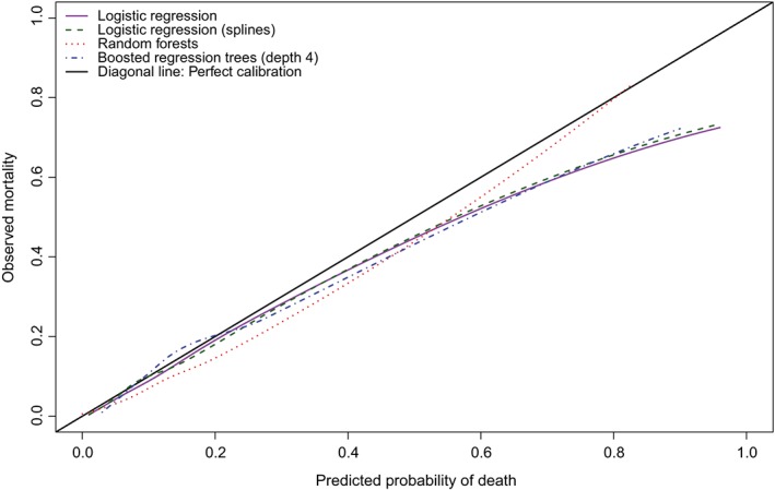
Calibration in validation sample (loess) (Figure 1 is a modification of a previously‐published figure12)[Colour figure can be viewed at wileyonlinelibrary.com]

The values of the calibration metrics for the four prediction methods when applied to the validation sample are reported in Table 1. Based on the E_max statistic, random forests resulted in predictions that displayed substantially better calibration than the other three methods, with the maximum difference between observed and predicted probabilities being 0.066, while logistic regression with linear main effects had the worst calibration, with an E_max of 0.238. Based on the ICI and the E50, the logistic regression model that incorporated restricted cubic splines had the best calibration; however, its values of these two metrics were only negligibly lower than that of the logistic regression model with linear effects. The value of the E90 was lowest for the logistic regression model with linear effects; however, its value of the E90 was only negligibly lower than that of the logistic regression model that incorporated restricted cubic splines. The mean weighted difference between observed and predicted probabilities was 38% smaller for the logistic regression model incorporating restricted cubic splines than for the boosted regression trees of depth four, while it was 52% smaller than for the random forest. Note that the 95% confidence intervals for the E_max metric were substantially larger than the 95% confidence intervals for the other three metrics, indicating greater uncertainty in the estimates of E_max compared to that of the other metrics.

Table 1.

Calibration metrics and associated 95% confidence intervals in the validation sample

Calibration	Logistic	Logistic regression	Random forests	Boosted regression
metric	regression with	with restricted		trees of depth four
	linear effects	cubic splines
ICI	0.014	0.013	0.027	0.021
	(0.008, 0.024)	(0.008, 0.023)	(0.020, 0.036)	(0.015, 0.029)
E50	0.007	0.006	0.024	0.019
	(0.003, 0.014)	(0.002, 0.011)	(0.007, 0.032)	(0.013, 0.024)
E90	0.023	0.024	0.063	0.039
	(0.009, 0.065)	(0.01, 0.073)	(0.046, 0.098)	(0.020, 0.071)
Emax	0.238	0.227	0.066	0.182
	(0.083, 0.452)	(0.076, 0.437)	(0.054, 0.239)	(0.066, 0.384)

Note: Each cell contains the appropriate calibration metric and its 95% confidence interval.

Abbreviation: ICI, Integrated Calibration Index.

The 95% confidence intervals for the calibration metrics reported in Table 1 were constructed using bootstrap methods. The following procedure was used: (i) a bootstrap sample was drawn from the derivation sample; (ii) a bootstrap sample was drawn from the validation sample; (iii) the given prediction method was fit to the bootstrap sample drawn from the derivation sample; (iv) the prediction method developed in the derivation sample in the previous step was applied to the bootstrap sample drawn from the validation sample; (v) each of the four calibration metrics was assessed in the bootstrap sample drawn from the validation sample for the prediction method developed in the third step. Two thousand bootstrap replicates were used (ie, steps (i) to (v) were conducted 2000 times). Percentile‐based bootstrap confidence intervals were then constructed using these 2000 bootstrap replications. Thus, for a given calibration metric and prediction method, the endpoints of the estimated 95% confidence interval were the empirical 2.5th and 97.5th percentiles of the distribution of the given calibration metric across the 2000 bootstrap replicates.

Pairwise differences between calibration metrics and associated 95% confidence intervals for these differences are reported in Table 2. The approach for computing 95% confidence intervals was similar to that described in the previous paragraph. We infer that two prediction methods had comparable performance on a given calibration metric if the 95% confidence included zero. The four prediction methods all had comparable calibration when assessed using E_max. When using the ICI and E50, the two logistic regression‐based methods had superior calibration compared to the two tree‐based methods.

Table 2.

Difference in calibration metrics (95% confidence interval) between different prediction methods

Method	Logistic regression with	Logistic regression	Random forests	Boosted regression
	linear effects	with RCS		trees of depth four
ICI
Logistic regression with	0 (0,0)	0.001	−0.013	−0.007
linear effects		(−0.005, 0.004)	(−0.019, −0.007)	(−0.016, 0)
Logistic regression with	−0.001	0 (0, 0)	−0.014	−0.008
RCS	(−0.004, 0.005)	(−0.02, −0.006)	(−0.015, 0)
Random forests	0.013 (0.007, 0.019)	0.014	0 (0, 0)	0.006
		(0.006, 0.02)		(−0.004, 0.014)
Boosted regression trees	0.007	0.008	‐0.006	0 (0, 0)
	(0, 0.016)	(0, 0.015)	(−0.014, 0.004)
E50
Logistic regression with	0 (0, 0)	0.001	−0.017	−0.012
linear effects		(−0.003, 0.007)	(−0.024, 0)	(−0.016, −0.004)
Logistic regression with	−0.001	0 (0,0)	−0.018	−0.013
RCS	(−0.007, 0.003)		(−0.025, −0.001)	(−0.018, −0.006)
Random forests	0.017	0.018	0 (0, 0)	0.005
	(0, 0.024)	(0.001, 0.025)		(−0.012, 0.014)
Boosted regression trees	0.012	0.013	−0.005	0 (0, 0)
	(0.004, 0.016)	(0.006, 0.018)	(−0.014, 0.012)
E90
Logistic regression with	0 (0, 0)	−0.001	−0.04	−0.016
linear effects		(−0.024, 0.015)	(−0.064, −0.015)	(−0.036, 0.022)
Logistic regression with	0.001	0 (0, 0)	−0.039	−0.015
RCS	(−0.015, 0.024)		(−0.061, −0.008)	(−0.032, 0.026)
Random forests	0.04	0.039	0 (0, 0)	0.024
	(0.015, 0.064)	(0.008, 0.061)		(0.005, 0.057)
Boosted regression trees	0.016	0.015	−0.024	0 (0, 0)
(−0.022, 0.036)	(−0.026, 0.032)	(−0.057, −0.005)
Emax
Logistic regression with	0 (0, 0)	0.011	0.172	0.056
linear effects		(−0.137, 0.151)	(−0.046, 0.343)	(−0.121, 0.23)
Logistic regression with	−0.011	0 (0, 0)	0.161	0.045
RCS	(−0.151, 0.137)		(−0.049, 0.334)	(−0.107, 0.208)
Random forests	−0.172	−0.161	0 (0, 0)	−0.116
	(−0.343, 0.046)	(−0.334, 0.049)		(−0.257, 0.08)
Boosted regression trees	−0.056	−0.045	0.116	0 (0, 0)
	(−0.23, 0.121)	(−0.208, 0.107)	(−0.08, 0.257)

Each cell reports the difference between the given metric for the method in the given row and the method in the given column (row method – column method) and associated 95% confidence interval. Negative values imply that the method in the given row has superior calibration than the method in the given column.

Abbreviations: ICI, Integrated Calibration Index; RCS, restricted cubic splines.

We conducted a further set of analyses to examine whether the statistical method used to estimate the calibration curve had an impact on the estimated calibration metrics. As noted above, our impression is that the most common approach is to use a locally weighted scatter plot smoother, such as a locally weighted least squares regression smoother. We considered two different R functions for implementing this: loess and lowess (loess is newer with different defaults). We used loess(Y∼P) and lowess(Y∼P,iter = 0), where Y denotes the observed binary outcome and P denotes the predicted probability. We also considered a method based on using a logistic regression model and restricted cubic splines.2 We used logistic regression to regress the observed binary outcome on the estimated predicted probability of the outcome, using restricted cubic splines to model the relation between the predicted probabilities and the log odds of the outcome. We used the probabilities themselves rather than the log odds of the probabilities, since the random forest method resulted in some predicted probabilities of zero, for which the log odds is undefined. We used restricted cubic splines with either 3 or 4 knots (the larger of the two for which there were no numerical estimation problems). The calibration curves for the second and third methods are reported in Figures 2 and 3, respectively. The calibration metrics for the different methods of estimating calibration curves are reported in Table 3. For a given performance metric and prediction method, differences between the two different implementations of a locally weighted scatter plot smoother tended to be minimal. Differences between the two implementations of this approach were the greatest for E_max. For the logistic regression model with linear effects, the two values of E_max were 0.238 and 0.158. The use of locally weighted scatter plot smoothing methods and the use of restricted cubic splines to estimate the calibration curve tended to result in similar values of the calibration metrics. Regardless of how the calibration curve was estimated, random forests had the lowest value of E_max. Again, differences between the methods were most evident for E_max. Regardless of how the calibration curve was estimated, one of the two logistic regression models had the lowest value of ICI, E50, and E90 (with minimal differences between the values of the calibration metric between the two logistic regression‐based approaches).

Figure 2.

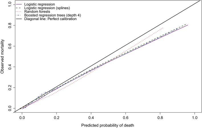
Calibration in validation sample (lowess) [Colour figure can be viewed at wileyonlinelibrary.com]

Figure 3.

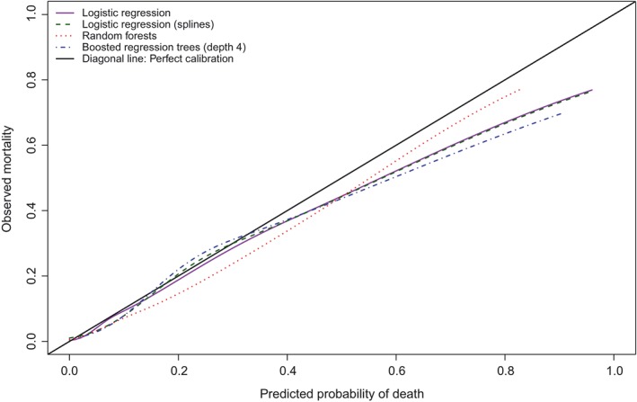
Calibration in validation sample (logistic regression with restricted cubic splines) [Colour figure can be viewed at wileyonlinelibrary.com]

Table 3.

Calibration metrics for three different methods of producing calibration curves

Metric	Logistic regression	Logistic regression with	Random	Boosted
	with linear effects	restricted cubic splines	forests	regression trees
loess function for estimating calibration curve
ICI	0.014	0.013	0.027	0.021
E50	0.007	0.006	0.024	0.019
E90	0.023	0.024	0.063	0.039
Emax	0.238	0.227	0.066	0.182
lowess function for estimating calibration curve
ICI	0.013	0.012	0.026	0.020
E50	0.007	0.006	0.022	0.018
E90	0.026	0.025	0.058	0.033
Emax	0.158	0.148	0.061	0.142
Restricted cubic spline for estimating calibration curve
ICI	0.013	0.015	0.027	0.021
E50	0.010	0.009	0.021	0.016
E90	0.019	0.023	0.061	0.025
Emax	0.193	0.195	0.063	0.209

Abbreviation: ICI, Integrated Calibration Index.

Harrell's E_max(a, b) metric denotes the maximum difference between observed and predicted probabilities within a subinterval of the unit interval. This allows for a quantification of calibration within specified risk intervals. A similar restriction can be implemented with each of the calibration methods. We categorized subjects in the validation sample into low‐risk, medium‐risk, and high‐risk strata, based on the following (admittedly subjective) thresholds: subjects whose predicted probability was less than or equal to 0.05 were classified as low‐risk, subjects whose predicted probability was greater than 0.05 and less than or equal to 0.10 were classified as medium‐risk, while subjects whose predicted probabilities exceeded 0.10 were classified as high‐risk. The values of the four calibration metrics for each of the four prediction methods within each of the three risk strata are reported in Table 4. Within the low‐risk stratum, the value of the ICI was comparable for the two logistic regression‐based approaches and for the random forest. In the medium‐risk stratum, the use of logistic regression that incorporated restricted cubic splines had the best performance for all four calibration metrics. In the high‐risk stratum, the two logistic regression‐based approaches had the lowest values of the ICI, E50, and E90.

Table 4.

Calibration metrics in low, medium, and high risk strata

Metric	Logistic regression	Logistic regression with	Random	Boosted
	with linear effects	restricted cubic splines	forests	regression trees
Low risk subjects (predicted probability ≤0.05)
ICI	0.007	0.006	0.006	0.019
E50	0.007	0.006	0.005	0.020
E90	0.007	0.007	0.014	0.022
Emax	0.007	0.007	0.019	0.022
Medium risk subjects (predicted probability 0.05 to 0.10)
ICI	0.009	0.003	0.025	0.006
E50	0.009	0.003	0.026	0.005
E90	0.011	0.005	0.029	0.011
Emax	0.012	0.005	0.030	0.012
High risk subjects (predicted probability >0.10)
ICI	0.026	0.028	0.052	0.035
E50	0.012	0.020	0.056	0.021
E90	0.060	0.062	0.066	0.080
Emax	0.238	0.227	0.066	0.182

Abbreviation: ICI, Integrated Calibration Index.

Finally, for comparative purposes, we used the Hosmer‐Lemeshow test to test the null hypothesis of model fit.13 The p‐values for testing the null hypothesis of model fit for the logistic regression model with linear main effects, the logistic regression model with restricted cubic splines, the random forests, and the boosted regression trees were 0.0035, 0.0043, <0.0001, and <0.0001, respectively. Thus, based on the Hosmer‐Lemeshow test, we would reject the null hypothesis of model fit. The Hosmer‐Lemeshow test is a formal statistical test of model fit and lacks further interpretation. In comparison, the methods described in the current study are descriptive methods for quantifying the magnitude of differences between observed and predicted probabilities. The Hosmer‐Lemeshow test does not provide a quantification of the magnitude of the lack of calibration.

Code for computing the ICI, E50, and E90 using the R statistical programming language is provided in the Appendix.

4. MONTE CARLO SIMULATIONS

We conducted two sets of Monte Carlo simulations to study the behavior of the four different calibration metrics for summarizing graphical calibration curves and of three different methods for producing calibration curves. In the first set of simulations, there was a true quadratic relation between a continuous covariate and the log odds of the binary outcome. In the second set of simulations, there was an interaction between two continuous covariates. In each set of simulations, we fit both a correctly specified model and an incorrectly specified model.

4.1. Design of Monte Carlo simulations

We simulated derivation and validation data from the same population. We considered two different logistic regression models that related a binary outcome to continuous covariates.

4.1.1. Simulation 1: quadratic relationship

We simulated derivation and validation samples of size N (see below for the values of N). For each subject in each of the two samples, we simulated a continuous covariate from a standard normal distribution: x_i ∼ N(0, 1). For each subject, a linear predictor was defined as ${\text{LP}}_i=x_i+a_2{x}_i^2$ (see below for the values of a ₂). Then, a binary outcome was simulated from a Bernoulli distribution: Y_i = Be(p_i), where $p_i=\frac{\text{exp}\left({\text{LP}}_i\right)}{1+\text{exp}\left({\text{LP}}_i\right)}$. Two logistic regression models were then fit to the simulated derivation sample: (i) a correctly specified regression model in which the binary outcome was regressed on both the continuous covariate and the square of the continuous covariate; (ii) an incorrectly specified regression model in which the binary outcome was regressed on only the continuous covariate (and the quadratic term was omitted). Each of the two fitted regression models was then applied to the simulated validation sample and predicted probabilities of the occurrence of the outcome were estimated for each subject in the validation sample. The three methods described above were then used to compute calibration curves in the validation sample (use of the R functions loess and lowess, and the use of logistic regression with restricted cubic splines). Each of the four calibration metrics (ICI, E50, E90, and E_max) was computed using each of the three calibration curves. This process was repeated 1000 times. For each method of estimating the calibration curve, the mean of each calibration metric was computed across the 1000 simulation replicates.

The size of the simulated data sets (N) was allowed to take on three values: 1000, 2000, and 5000. The regression coefficient (a ₂) for the quadratic term was allowed to take on 10 values: from 0.1 to 1, in increments of 0.1. We used a full factorial design and hence considered 30 different scenarios.

4.1.2. Simulation 2: interactions

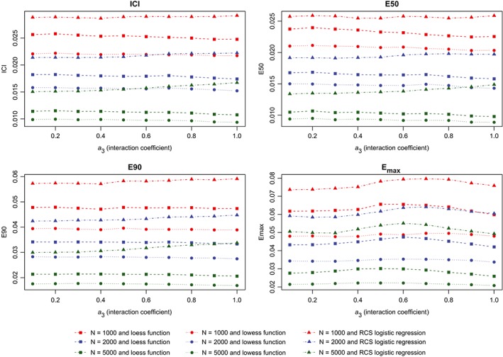
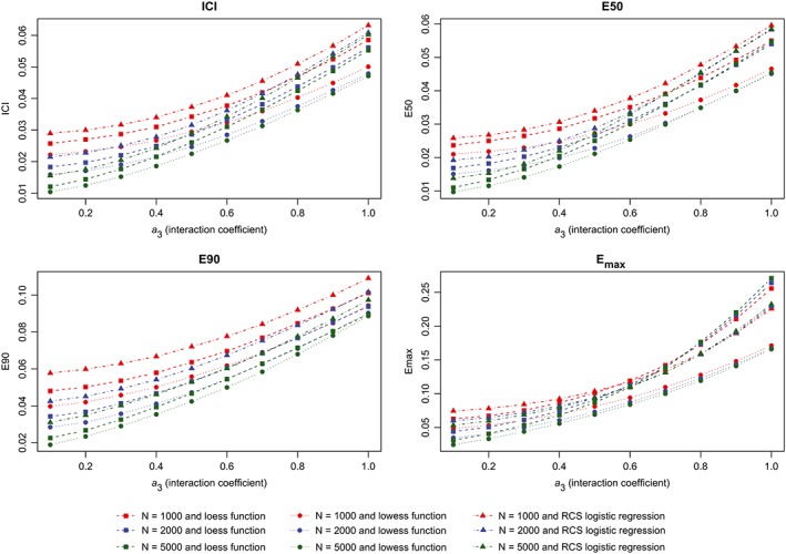
The second set of simulations was similar to the first, except that the logistic regression model included an interaction between two continuous covariates. For each subject, we simulated two continuous covariates, x_1i and x_2i, from independent standard normal distributions. The linear predictor used to generate outcomes was LP_i = x_1i + x_2i + a₃x_1ix_2i. In the simulated derivation sample, we fit two models: (i) a correctly specified logistic regression model in which the binary outcome was regressed on the two covariates and their interaction and (ii) an incorrectly specified logistic regression model in which the binary outcome was regressed on only the two covariates (and the interaction was omitted). Apart from these design differences, this second set of simulations was identical to the first set.

The size of the simulated data sets (N) was allowed to take on three values: 1000, 2000, and 5000. The regression coefficient (a ₃) for the interaction term was allowed to take on 10 values: from 0.1 to 1, in increments of 0.1. We used a full factorial design and hence considered 30 different scenarios.

4.2. Results of Monte Carlo simulations

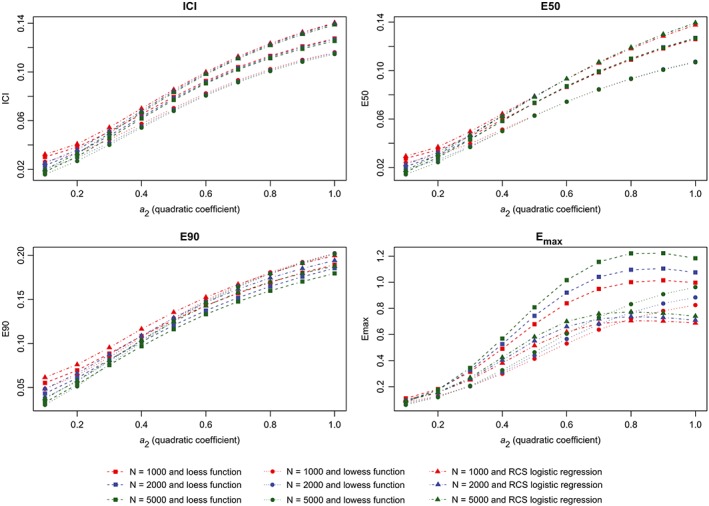
The results of the first set of simulations are reported in Figure 4 (calibration metrics for the correctly specified regression model), Figure 5 (calibration metrics for the incorrectly specified model), and Figure 6 (differences in calibration metrics between the correctly specified and incorrectly specified models). When the correctly specified model was fit, each calibration metric decreased toward zero with increasing sample size. In general, for a given sample size, the use of the lowess function to estimate the calibration curve resulted in the lowest value of a given calibration metric, while the use of a logistic regression model with restricted cubic splines resulted in the highest value of a given calibration metric. The effect of increasing sample size was greatest on E_max. When the incorrectly specified model was fit, the mean value of each calibration metric increased with degree of misspecification (as measured by the magnitude of the coefficient for the quadratic term) (Figure 5). Similarly, the difference in a given performance metric between the correctly specified and incorrectly specified regression models increased with degree of misspecification (Figure 6).

Figure 4.

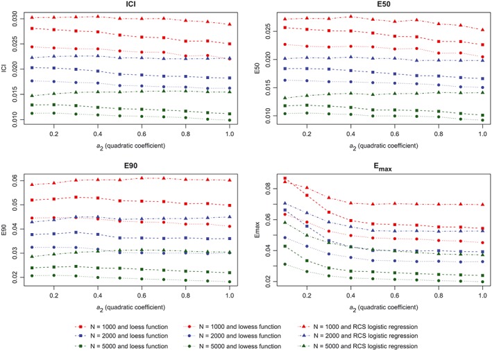
Metrics for correctly specified model (quadratic). ICI, Integrated Calibration Index [Colour figure can be viewed at wileyonlinelibrary.com]

Figure 5.

Metrics for incorrectly specified model (quadratic). ICI, Integrated Calibration Index [Colour figure can be viewed at wileyonlinelibrary.com]

Figure 6.

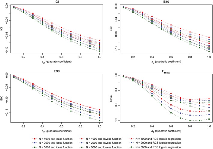
Change in metrics between two models (quadratic). ICI, Integrated Calibration Index [Colour figure can be viewed at wileyonlinelibrary.com]

The results of the second set of simulations are reported in Figure 7 (calibration metrics for the correctly specified regression model), Figure 8 (calibration metrics for the incorrectly specified model) and Figure 9 (differences in calibration metrics between the correctly specified and incorrectly specified models). The results were similar to those observed for the first set of simulations.

Figure 7.

Metrics for correctly specified model (interaction). ICI, Integrated Calibration Index [Colour figure can be viewed at wileyonlinelibrary.com]

Figure 8.

Metrics for incorrectly specified model (interaction). ICI, Integrated Calibration Index [Colour figure can be viewed at wileyonlinelibrary.com]

Figure 9.

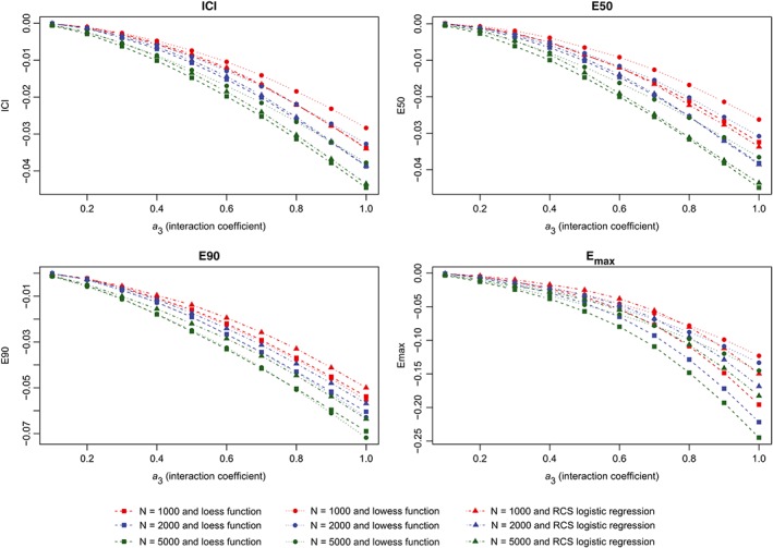
Change in metrics between two models (interaction). ICI, Integrated Calibration Index [Colour figure can be viewed at wileyonlinelibrary.com]

5. DISCUSSION

We have described the ICI, which is a simple numerical method for quantifying the calibration of methods for predicting probabilities of the occurrence of a binary outcome. The ICI is the weighted mean difference between observed and predicted probabilities of the occurrence of the outcome, where differences are weighted by the empirical density function of predicted probabilities. An advantage of the proposed metric is that it provides a numeric summary of differences between observed and predicted probabilities across the entire range of predicted probabilities in a way that accounts for the distribution of predicted probabilities.

The greatest utility of the ICI and related measures such as E50 and E90 is for comparing the relative calibration of different prediction methods. When comparing different prediction methods, these measures allow for a quantitative assessment of which method has the best calibration. While our primary intent is that these metrics will facilitate choosing the best performing prediction method from a set of candidate prediction methods, it is possible that these metrics can be used to evaluate a single prediction method in isolation. However, to do so would require specification of the maximum acceptable value of the ICI (or of E50 or E90). This value would likely depend on the clinical context and on the costs associated with inaccurate predictions. We would argue that there is not a single universal threshold of the ICI that denotes acceptable calibration. Our suggestion to use these calibration metrics to compare the relative calibration of different prediction methods is similar in spirit to a miscalibration index proposed by Dalton that was an extension of the method proposed by Cox that was described in the Introduction.14 Dalton defined a miscalibration ratio to be the ratio of the miscalibration indices for two different prediction methods; this ratio allows one to determine the relative decrease in miscalibration for one method compared to a competing method. The impact of miscalibration on decision making can be examined in more detail with a measure such as Net Benefit or Relative Utility.15, 16

Our ICI is motivated by Harrell's E_max statistic, which is the maximal absolute difference between the smoothed calibration curve and the diagonal line denoting best fit.3 Similarly, Harrell provides a one‐sentence suggestion that the average absolute difference between observed and predicted probabilities can be used.3 While not described or evaluated in the peer‐reviewed literature, E90 and E_avg (which is equivalent to our ICI metric) have been implemented in the rms package for the R statistical programming language.17 E_avg and ICI use the mean as the measure of central tendency for summarizing the absolute differences in between predicted and observed probabilities. We also proposed E50, in which the median is used to summarize absolute differences between predicted and observed probabilities. By using the median, E50 will be less influenced by a small minority of subjects for whom there is a large discrepancy between observed and predicted probabilities. By using the 90th percentile of the distribution of absolute differences between observed and predicted probabilities, we are able to summarize the limit to the absolute discrepancy for the large majority of subjects in the sample.

There are several advantages to the ICI and E50. First, like E_max(a, b), they provide a simple numeric summary of calibration. They thereby provide a simple method to compare the calibration of competing prediction models. Second, they have a simple interpretation as the weighted mean or median difference between observed and predicted probabilities. Third, because they provide a single numeric summary, they permit comparison of calibration reported in different studies. If the distribution of predicted probabilities differed between studies, this could complicate comparison of the ICI or E50 between studies. However, if individual patient data were available for the different studies, a form of standardization could be performed so that an “adjusted” ICI or E50 could be computed using the distribution of the predicted probabilities from one study as the reference distribution. Fourth, unlike a graphical assessment of calibration, they explicitly incorporate the distribution of the predicted probabilities and assign greater weight to differences where predicted probabilities are more common compared to differences where predicted probabilities are less common. Unlike graphical calibration curves, which readers can be tempted to interpret as though predicted probabilities were uniformly distributed across the unit interval, the ICI and E50 explicitly incorporate the distribution of the predicted probabilities into its calculation. Fifth, when comparing the calibration of competing prediction methods, they do not require that the range of predicted probabilities be the same for all methods. Since they integrate over the empirical distribution of predicted probabilities, they allow for a comparison of calibration between methods that result in different ranges of predicted probabilities. Sixth, as was observed in our case study, they can permit the identification of differences in calibration that are not possible from a naïve visual inspection of the graphical calibration curves.

Calibration curves can be difficult to interpret in isolation because, while the calibration curve is plotted over the entire empirical range of the predicted probabilities, the empirical distribution of predicted probabilities is frequently not uniform. A partial remedy for this limitation is to superimpose on the figure a depiction of the density function of the probabilities (or to display this in a panel directly under the calibration curve). Similarly, shaded confidence bands for the calibration curve can be added the graph to illustrate uncertainty in the calibration curve. While these additions can aid in the interpretation of calibration curves, the metrics examined in the current study permit a quantification of calibration and facilitate the comparison of the calibration of different prediction methods.

Harrell proposed the metric E_max(a, b), which denotes the maximum difference between predicted and observed probabilities over the interval (a, b).3 As illustrated in the case study, each of the four calibration metrics considered in the current study (ICI [or E_avg], E50, E90, and E_max) can be evaluated over a restricted interval rather than over the unit interval (0, 1). We would argue that, in most scenarios, one would be interested in the value of the calibration metric when evaluated over the entire range of predicted probabilities rather than over a restricted interval. When evaluated over the entire unit interval, the given calibration metric describes model performance in the entire validation sample. This is similar to the area under the Receiver Operating Characteristic curve quantifying discrimination over the full range of potential decision thresholds. In specific settings, one may be particularly interested in model performance in a subset of patients, such as those subjects with a high predicted probability of the outcome. In some clinical scenarios, miscalibration for low risk subjects may be of less importance than miscalibration for the smaller number of high‐risk subjects. In such settings, estimating the calibration metrics within an interval denoting high‐risk may be the preferred approach.

When comparing the calibration of two prediction models, it is possible that they may have the same calibration, as quantified by the ICI. Thus, on average, the difference between predicted and observed probabilities of the outcome is similar for the two methods. However, the two methods may differ in the region in the risk dimension in which miscalibration occurs. For instance, one method may display better calibration in low‐risk subjects and poorer calibration in high‐risk subjects, while the other method may display poorer calibration in low‐risk subjects and better calibration in high‐risk subjects. Evaluating the different calibration metrics within different subintervals of the unit interval will permit a more comprehensive comparison of the two methods. In our case study, we found that logistic regression‐based approaches tended to have superior calibration in low‐risk, medium‐risk, and high‐risk subjects compared to the two competing tree‐based methods. Decision curve analysis may be preferred when assessing the clinical usefulness of a prediction model, reflecting the impact of discrimination and calibration for a range of relevant decision thresholds.18

In summary, the ICI, which is weighted average of the absolute mean difference between a smoothed calibration curve and the diagonal line of perfect calibration, provides a single numeric summary of calibration. It has a simple and intuitively appealing interpretation. Its use in studies validating prediction models will enhance comparisons of the relative performance of different prediction methods. Its value can be simultaneously reported with graphical displays of calibration and its companion metrics E50 and E90.

R CODE FOR COMPUTING THE ICI

# This code is provided for illustrative purposes and comes with ABSOLUTELY NO

# WARRANTY.

# Let Y denote a vector of observed binary outcomes.

# Let P denote a vector of predicted probabilities.

loess.calibrate <‐ loess(Y ∼ P)

# Estimate loess‐based smoothed calibration curve

P.calibrate <‐ predict (loess.calibrate, newdata = P)

# This is the point on the loess calibration curve corresponding to a given predicted probability.

ICI <‐ mean (abs(P.calibrate – P))

# The value of the ICI

E50 <‐ median (abs(P.calibrate – P))

E90 <‐ quantile (abs(P.calibrate – P), probs = 0.9)

Emax <‐ max (abs(P.calibrate – P))

Austin PC, Steyerberg EW. The Integrated Calibration Index (ICI) and related metrics for quantifying the calibration of logistic regression models. Statistics in Medicine. 2019;38:4051–4065. 10.1002/sim.8281

REFERENCES

- 1. Cox DR. Two further applications of a model for binary regression. Biometrika. 1958;45(3‐4):592‐565. 10.1093/biomet/45.3-4.562 [DOI] [Google Scholar]
- 2. Van Calster B, Nieboer D, Vergouwe Y, De CB, Pencina MJ, Steyerberg EW. A calibration hierarchy for risk models was defined: from utopia to empirical data. J Clin Epidemiol. 2016;74:167‐176. 10.1016/j.jclinepi.2015.12.005 [DOI] [PubMed] [Google Scholar]
- 3. Harrell FE Jr. Regression Modeling Strategies: With Applications to Linear Models, Logistic Regression, and Survival Analysis. New York, NY: Springer‐Verlag; 2001. [Google Scholar]
- 4. Steyerberg EW. Clinical Prediction Models: A Practical Approach to Development, Validation, and Updating. New York, NY: Springer‐Verlag; 2009. [Google Scholar]
- 5. Austin PC, Steyerberg EW. Graphical assessment of internal and external calibration of logistic regression models by using loess smoothers. Stat Med. 2014;33(3):517‐535. 10.1002/sim.5941 [DOI] [PMC free article] [PubMed] [Google Scholar]
- 6. Breiman L. Random forests. Machine Learning. 2001;45(1):5‐32. [Google Scholar]
- 7. Buhlmann P, Hathorn T. Boosting algorithms: regularization, prediction and model fitting. Statistical Science. 2007;22:477‐505. [Google Scholar]
- 8. Freund Y, Schapire R. Experiments with a new boosting algorithm. In: Proceedings of the Thirteenth International Conference on International Conference on Machine Learning; 1996; San Francisco, CA. [Google Scholar]
- 9. Friedman J, Hastie T, Tibshirani R. Additive logistic regression: a statistical view of boosting (with discussion). Ann Stat. 2000;28:337‐407. [Google Scholar]
- 10. Hastie T, Tibshirani R, Friedman J. The Elements of Statistical Learning. New York, NY: Springer; 2009. [Google Scholar]
- 11. Cleveland WS, Grosse E, Shyu WM. Local regression models In: Chambers JM, Hastie TJ, eds. Statistical Models in S. New York, NY: Chapman & Hall; 1993:309‐376. [Google Scholar]
- 12. Austin PC, Lee DS, Steyerberg EW, Tu JV. Regression trees for predicting mortality in patients with cardiovascular disease: what improvement is achieved by using ensemble‐based methods? Biom J. 2012;54(5):657‐673. 10.1002/bimj.201100251 [DOI] [PMC free article] [PubMed] [Google Scholar]
- 13. Hosmer DW, Lemeshow S. Applied Logistic Regression. New York, NY: John Wiley & Sons; 1989. [Google Scholar]
- 14. Dalton JE. Flexible recalibration of binary clinical prediction models. Statist Med. 2013;32(2):282‐289. [DOI] [PubMed] [Google Scholar]
- 15. Steyerberg EW, Vickers AJ, Cook NR, et al. Assessing the performance of prediction models: a framework for traditional and novel measures. Epidemiology. 2010;21(1):128‐138. [DOI] [PMC free article] [PubMed] [Google Scholar]
- 16. Van CB, Vickers AJ. Calibration of risk prediction models: impact on decision‐analytic performance. Med Decis Mak. 2015;35(2):162‐169. 10.1177/0272989X14547233 [DOI] [PubMed] [Google Scholar]
- 17. rms: Regression Modeling Strategies. https://cran.r-project.org/web/packages/rms/index.html
- 18. Vickers AJ, Van CB, Steyerberg EW. Net benefit approaches to the evaluation of prediction models, molecular markers, and diagnostic tests. BMJ. 2016;352:i6 10.1136/bmj.i6 [DOI] [PMC free article] [PubMed] [Google Scholar]