PyFrag 2019—Automating the exploration and analysis of reaction mechanisms

Abstract

We present a substantial update to the PyFrag 2008 program, which was originally designed to perform a fragment‐based activation strain analysis along a provided potential energy surface. The original PyFrag 2008 workflow facilitated the characterization of reaction mechanisms in terms of the intrinsic properties, such as strain and interaction, of the reactants. The new PyFrag 2019 program has automated and reduced the time‐consuming and laborious task of setting up, running, analyzing, and visualizing computational data from reaction mechanism studies to a single job. PyFrag 2019 resolves three main challenges associated with the automated computational exploration of reaction mechanisms: it (1) computes the reaction path by carrying out multiple parallel calculations using initial coordinates provided by the user; (2) monitors the entire workflow process; and (3) tabulates and visualizes the final data in a clear way. The activation strain and canonical energy decomposition results that are generated relate the characteristics of the reaction profile in terms of intrinsic properties (strain, interaction, orbital overlaps, orbital energies, populations) of the reactant species. © 2019 The Authors. Journal of Computational Chemistry published by Wiley Periodicals, Inc.

Introduction

In recent decades, significant progress has been made in the field of quantum chemistry,1, 2 especially toward the development of density functional theory methods.3, 4, 5 In combination with the vast increase in computational resources now available to researchers, chemical modeling has become a modern discipline. Indeed, nowadays computational chemistry programs allow not only the modeling of a large variety of chemical systems and processes with sufficient accuracy,6, 7, 8, 9 but they also provide a better, more thorough understanding of chemical phenomena, based on first principles.10, 11, 12 The obtained insight and understanding of a given reaction mechanism can then be used for the systematic optimization of reaction conditions and other parameters, thereby enhancing the efficiency of the chemical reaction and reducing unwanted side products.13, 14 Computational insight, thus, greatly enhances the capabilities of the chemists and provides them with an additional and often complementary perspective to tackle chemical problems with little limitations from experimental conditions.15, 16

A number of theoretical models have been developed to analyze different aspects of chemical reactions and the associated changes in the chemical bonding situation. Examples are frontier molecular orbital (FMO) theory,17, 18 Marcus theory,19, 20 and the curve‐crossing model in valence bond (VB) theory.21, 22 An even more extensive analysis technique is the Activation Strain Model23 (ASM), also known as the distortion/interaction model.24, 25 The ASM is a fragment‐based approach that characterizes reactions in terms of simple and intuitive concepts, such as the effect of geometrical deformations of the reactants and various interaction terms due to changes in the electronic structure along the reaction path. For instance, we have previously used the ASM to understand how the reaction barrier varies when different bonds are activated by palladium,26 or how ligands can change the activating capability of palladium,27 or how and why other metal centers perform differently in cross‐coupling reactions compared to palladium.28 In addition, the ASM has been successfully applied to understand the quantitative factors governing molecular reactivity in other systems like cycloadditions,29, 30, 31, 32, 33, 34, 35 metalorganic catalysis,11, 36, 37 and substitution reactions.38, 39, 40

The original version of PyFrag 200841 allowed for the routine exploration and analysis of potential energy surfaces using the ASM. That version consisted of a driver invoking the Amsterdam Density Functional (ADF) software,42, 43, 44 which in turn made use of the concept of molecular fragments for the analysis of chemical bonds.12 After many successful applications, we have now overhauled the original PyFrag 2008 code with the aim to (1) make extensive usage of the scripting framework provided by the Python Library for Automating Molecular Simulations (PLAMS)45 and QMflows;46 thereby enabling PyFrag 2019 to (2) be compatible with other quantum chemistry programs such as Gaussian,47 Orca,48 and Turbomole49 and their respective analysis tools; and (3) completely automate the workflow of the ASM approach. In order to monitor the computational progress at runtime, PyFrag 2019 uses Bokeh,50 an interactive visualization Python library, to generate an html file summarizing the computational results in tables, figures, and videos.

PyFrag 2019 requires the user to simply supply approximate geometries of the stationary points (reactants, transition states, and products). PyFrag 2019 then sets up and runs the optimizations of the stationary points and also the complex workflows associated with the ASM approach involving many calls to computational chemistry programs in sequential order or, where possible, in parallel. The computational progress and the convergence of the required geometry and transition state optimizations can be monitored at runtime. After completing the computations, PyFrag 2019 then visualizes the results in a clear, automated, and informative way.

The remainder of this article is organized as follows: the subsequent section describes the ASM and energy decomposition analysis (EDA) method, which are used to analyze properties and quantities along the reaction path. Afterward, we provide specific examples of the complete workflow as implemented in PyFrag 2019 being employed to understand the reactivity of, among many others tested, three widely studied reactions: the oxidative addition of C–X bonds by iron catalyst,28 1,3‐dipolar cycloaddition reactions,29 and the analysis of the nucleophilicity and leaving‐group ability of backside S_N2 reactions.38

Methods

The ASM is a fragment‐based approach used to understand the character of the reaction mechanism and to gain insights into the overall reaction energy profile. Usually, the reaction profile is determined by the interplay between two reactants or fragments. The bonding energy ΔE is decomposed along the intrinsic reaction coordinate (IRC)51, 52 into the strain energy ΔE _strain that is associated with the geometrical deformation of the individual reactants as the process takes place, plus the actual interaction energy ΔE _int between the deformed reactants (see eq. 1).

$$\mathrm{\Delta }E=\mathrm{\Delta }{E}_{\text{strain}}+\mathrm{\Delta }{E}_{\mathrm{int}}$$ (1)

The interaction energy ΔE _int between the deformed reactants is further analyzed in the conceptual framework provided by the Kohn‐Sham molecular orbital (KS‐MO) model, using a quantitative EDA scheme (eq. 2).12, 53, 54, 55 While any of the aforementioned computational chemistry programs can be used to perform the activation strain analysis, it should be noted that the EDA presented in this article is a unique feature of ADF.42, 43, 44

$$\mathrm{\Delta }{E}_{\mathrm{int}}=\mathrm{\Delta }{V}_{\text{elstat}}+\mathrm{\Delta }{E}_{\text{Pauli}}+\mathrm{\Delta }{E}_{\mathrm{oi}}$$ (2)

The ΔV _elstat energy corresponds to the classical Coulomb interaction between the unperturbed charge distributions of the deformed reactants and is usually attractive. The Pauli repulsion energy ΔE _Pauli comprises the destabilizing interactions between occupied orbitals (more precisely, between same‐spin spin orbitals) on the respective reactants and is responsible for steric repulsion. The orbital interaction energy ΔE _oi accounts for charge transfer (interaction between occupied orbitals on one fragment with unoccupied orbitals on the other fragment, including the HOMO–LUMO interactions) and polarization (empty‐occupied orbital mixing on one fragment due to the presence of another fragment).

Description of the Program

An overview of the complete PyFrag 2019 workflow is shown in Figure 1. Our new implementation consists of three parts: calculation and preparation of the whole reaction path, activation strain analysis based on this computed reaction path, and finally the tabulation and visualization of all results. The user only needs to provide basic information like initial guesses for the molecular structures and the specific parameters required for the DFT calculations (see the Supporting Information for an example input file). PyFrag 2019 then automatically submits the necessary computational jobs to (eventually remote) computing nodes and gathers the corresponding results after the completion of each job. The structures of the reactants and products of the reaction are optimized first, followed by a search for the transition state starting from a reasonable initial guess for its geometry. A frequency analysis is then performed to ensure that the previously optimized structures and the transition state are indeed stationary points on the potential energy surface. A deeper understanding of a reaction mechanism can often be gained only by inspecting the entire reaction path rather than the stationary points alone.56, 57 For this reason, a reaction path between the transition state and the initial and final structures, respectively, is then generated by means of an IRC calculation.51, 52 The activation strain analysis is then performed to identify the main mechanistic characteristics of a given reaction. During the execution of the workflow, relevant information about the current status is collected and written into an html output file, an example of which is depicted in Figure 2a‐c. Upon completion of the workflow, the activation strain diagram is generated (Fig. 2d). The activation strain analysis results are also collected and stored as a text file, which can be exported and plotted in MS Excel either manually or automatically with the help of a supplementary function in PyFrag 2019. In cases where the reaction path is already available, PyFrag 2019 is also able to import the coordinates and directly proceed with the activation strain analysis workflow using either ADF,42 Gaussian,47 ORCA,48 or Turbomole.49 ExcelAutomat 1.358 (compatible with Gaussian47 and GAMESS‐US59, 60, 61) and autoDIAS62 (compatible with Gaussian,47 ORCA,48 NWChem,63 and Q‐Chem64) have recently been published and have been shown to be useful in automating the activation strain analysis along a provided reaction coordinate. Note, however, that while making advances toward an automated process, both of these programs are incompatible with ADF and thus are unable to perform the EDA.12, 53, 54, 55 We should also note that the present version of PyFrag 2019 is not yet compatible with open‐shell calculations.

Figure 1.

Schematic flowchart of the PyFrag 2019 program, including the three steps of (i) preparations, (ii) analysis, and (iii) visualization. [Color figure can be viewed at wileyonlinelibrary.com]

Figure 2.

Snapshots from the html page generated by PyFrag 2019 that shows (a) the current job status (Transition State); (b) corresponding movies of each geometrical optimization process; (c) the summary of the geometries and energies of stationary points on the potential energy surface [reactant (R1), reactant complex (RC), transition state (TS), and product (P)]; and (d) after completion of the workflow, the results of the activation strain analysis. For the current job status, various types of information are provided, including: a plot of energy (E) against each step, convergence information like energy change (e), constrained gradient max (c_max), their responding converge standard (e_, c_max), as well as if they are converged (e_TF, gm_TF). The user can click the box and select other stationary points, such as the reactant or product and obtain relevant data. [Color figure can be viewed at wileyonlinelibrary.com]

To facilitate the rapid evaluation of the workflow and to display the status of the entire computation, PyFrag 2019 provides the functionality to periodically extract relevant data from the running calculation and visualize it as an html output (see Fig. 2). A continuously updated video can be generated to examine the reaction path in real time. In the case of a failure of a computation, such as geometry optimization, the workflow will continue carrying out all other computations, unless they explicitly depend on the job that has failed. When such erratic behavior occurs, the user can modify the input file, which in turn will be detected and accounted for by PyFrag 2019 and used to restart any affected computational jobs automatically.

Results and Discussion

To demonstrate the ability of PyFrag 2019 to automate the steps necessary for the mechanistic analysis summarized in Figure 1, we proceed by presenting three application cases involving different chemical reactions: an (1) oxidative addition to an iron catalyst, a (2) series of 1,3‐dipolar cycloadditions, and (3) bimolecular nucleophilic substitution (S_N2) reactions. In order to perform these analyses, as mentioned above, the user must only supply approximate geometries of the stationary points (reactants, transition state, and products). After completion of the calculation, the user can then plot the activation strain and EDA that were generated by PyFrag 2019 with the selected quantum chemistry program. In this section, we limit our discussion to the final step involving the visualization step, since this step of the workflow is the most informative for understanding the factors governing the reactivity of the specific reactions and to check the correct performance of PyFrag 2019.

Reaction 1: Oxidative addition by an iron catalyst

Catalytic reactions are a key transformation in modern synthetic chemistry65, 66 and the oxidative addition step is generally the first and rate‐determining step in most catalytic cycles.67, 68 Our first example involves the C─X bond activation via oxidative addition of CH₃X substrates (X = H, Cl, CH₃) to a model iron catalyst Fe(CO)₄ with singlet spin state.28 The results from the activation strain analysis carried out with PyFrag 2019 using ADF, Gaussian, ORCA, and Turbomole as computational engines are shown in Figure 3a‐d. As expected, but still important, we find comparable results and the same trends in reactivity for all programs employed, which confirms these individual implementations.

Figure 3.

Activation strain analysis for the oxidative addition of CH₃─X bonds (X=H, Cl, CH₃: black, blue, red, respectively) to singlet Fe(CO)₄ computed at (a) ZORA‐OPBE/TZ2P level with ADF 2017; (b) DKH‐OPBE/6–311++G(d,p) level with Gaussian 09; (c) ZORA‐OPBE/ZORA‐def2‐TZVP SARC/J level with ORCA 4.0; and (d) DKH‐BLYP/TZVP level with Turbomole 6.5. Energy barriers relative to the reactants for the transition state are included (see upper left corner) and the positions of TS are marked by diamonds. [Color figure can be viewed at wileyonlinelibrary.com]

The activation barrier (ΔE) depends on two chemically intuitive terms, namely the strain (ΔE _strain) and interaction (ΔE _int) energies (see eq. 1). We focus the following discussion on the results obtained with ADF as summarized in Figure 3a. The energy barriers for the bond activation of C─H, C─Cl, and C─C by Fe(CO)₄ increase from 10.4 to 25.5 to 48.0 kcal mol⁻¹, respectively. A weaker catalyst–substrate interaction results in a higher barrier for the C─Cl activation compared to the C─H activation. The C─C bond activation exhibits the highest barrier due to a highly destabilizing activation strain and a weakly stabilizing interaction energy compared to the activation of the C─H and the C─Cl bonds. The strength of the ΔE _int for these bond activation processes was traced back to the nature of the σ and σ* orbitals of the C─H, C─Cl or C─C bonds. In particular, the σ_{C─ H} lacks a nodal plane and has a significant overlap with the iron catalyst 3d _σ orbital in a σ‐donating manner. At variance, the σ_{C─ Cl} and σ_{C─ C} for C─Cl and C─C, respectively, have a 2p‐nodal plane that results in the cancellation of orbital overlap with the iron 3d _σ. These orbital overlap values are easily printed by PyFrag 2019 in the same manner as the activation stain terms. Finally, the more destabilizing ΔE _strain for C─C activation compared to C─Cl activation simply originates from the higher strength of the C─C bond.69

Reaction 2: 1,3‐dipolar cycloaddition reactions

Our second example investigates the 1,3‐dipolar cycloaddition (1,3‐DCA) reactivities of a series of aza‐1,3‐dipoles 1 (black), 2 (blue), 3 (red) with ethylene (e) as shown in Figure 4. 1,3‐DCA cycloadditions are important reactions in heterocyclic chemistry,70 materials chemistry,71, 72, 73 and chemical biology.74, 75, 76 The cycloaddition barrier increases from 1 to 2 to 3 corresponding to a sharp decrease in reactivity. Our activation strain analysis (Fig. 4a) reveals that the differences in the barrier heights for these 1,3‐DCA reactions originate from differences in ΔE _int and not from ΔE _strain, as originally proposed.25, 77, 78 Despite the reaction of 1 having the most destabilizing ΔE _strain, it goes with the lowest barrier due to a highly stabilizing ΔE _int. Decomposition of the interaction energy reveals that the trends in the Pauli repulsion, ΔE _Pauli, are more or less offset by the trends in the electrostatic interaction, ΔV _elstat (Fig. 4b). The orbital interactions, ΔE _oi, on the other hand, play a dominant role in determining the trend in interaction energy, and thus, the height of the reaction barriers. The orbital interaction becomes weaker from 1 to 2 to 3 due to a larger, less favorable FMO energy gaps. In addition, as the number of nitrogen atoms in the 1,3‐dipole increases from 1 to 3 for compounds 1, 2, and 3, respectively, the FMO overlap decreases, due to the more contracted 2p‐orbitals of nitrogen compared to those of carbon.79 These two effects, the larger FMO energy gaps and a decrease in FMO overlap, reinforce each other and result in a less stabilizing orbital interaction curve, and thus a higher and less favorable activation barrier.

Figure 4.

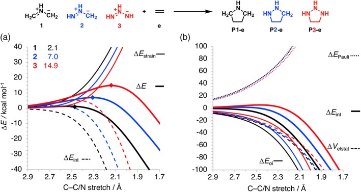
(a) Activation strain analyses and (b) energy decomposition analyses of the cycloaddition reactions between 1,3‐dipoles 1–3 and ethylene (e), computed at the BP86/TZ2P level. Energy barriers relative to the reactants for the transition state are included (see upper left corner), and the positions of TS are marked by diamonds. [Color figure can be viewed at wileyonlinelibrary.com]

Reaction 3: Bimolecular nucleophilic substitution (S_N2)

Our third example involves the textbook bimolecular nucleophilic substitution (S_N2) reaction.80 We have analyzed the nucleophilicity and leaving‐group ability of halogens in backside S_N2 reactions for X⁻ + CH₃Cl (X⁻ = F⁻, Cl⁻, Br⁻, and I⁻) and Cl⁻ + CH₃Y (Y = F, Cl, Br, and I), respectively.38 In Figure 5a, we show that for a given leaving group, the S_N2 barrier increases as the nucleophile is varied from F⁻ to I⁻. This trend stems entirely from the ΔE _int curves, as the ΔE _strain curves are nearly identical and superimposed. The nucleophilicity of these halides is determined by the electron‐donor capability of the nucleophile. Specifically, the HOMO–LUMO interaction becomes less stabilizing as the nucleophile is varied along X⁻ = F⁻, Cl⁻, Br⁻, and I⁻ and this, in turn, leads to a systematically less stabilizing interaction. This can be understood in terms of the orbital energy of the X⁻ HOMO, which is the highest (most destabilized) for F⁻ and decreases (becomes stabilized) to I⁻, thus leading to a larger HOMO–LUMO gap.

Figure 5.

Activation strain analysis of the S_N2 reactions for (a) X⁻ + CH₃Cl (X⁻ = F⁻, Cl⁻, Br⁻, and I⁻) and (b) Cl⁻ + CH₃Y (Y = F, Cl, Br, and I), computed at the OLYP/TZ2P level. Energy barriers relative to the reactants for the transition state are also included (see upper left corner), and the positions of TS are marked by diamonds. [Color figure can be viewed at wileyonlinelibrary.com]

For a given nucleophile, the S_N2 barrier decreases as the leaving group is varied from F to I for the Cl⁻ + CH₃Y (Y = F, Cl, Br, and I) reactions. Interestingly, in this case, the reactivity trend is entirely determined by the ΔE _strain curves, as the ΔE _int curves are nearly identical for the different reactions. The ΔE _strain curves become less destabilizing as the leaving group is varied from Y = F, Cl, Br, and I. The leaving group ability is directly related to the trend in C─Y bond strengths, with C─F being the strongest bond (ΔH _BDE = 113.7 kcal mol⁻¹) and C─I the weakest one (ΔH _BDE = 60.7 kcal mol⁻¹).81, 82

Conclusions

The PyFrag 2019 program is presented, featuring significant improvements over its predecessor,41 with the aim to facilitate the computational exploration and analysis of reaction mechanisms in an automated fashion. In particular, PyFrag 2019 resolves three main challenges associated with computing the potential energy surface of a particular reaction: it now (1) computes the reaction path by carrying out multiple parallel calculations using initial coordinates provided by the user; (2) monitors the entire workflow process; and (3) tabulates and visualizes the final data in a clear way. The automated activation strain analysis in PyFrag 2019 is compatible with many quantum chemical software packages, including ADF42, Gaussian47, Orca,48 and Turbomole.49

PyFrag 2019 requires the user to only provide approximate geometries for the respective stationary points on the potential energy surface (reactants, transition states, products, and intermediates). The steps of the reaction path workflow involve first running the geometry optimizations of stationary points using the supplied coordinates followed by an IRC calculation to generate the potential energy surface. Next, an activation strain and canonical EDA (when using ADF) is performed. The final step of the workflow involves the visualization (plotting/tabulation) of the results. These activation strain and energy decomposition results generated from PyFrag 2019 allow the user to relate the characteristics of the reaction profile in terms of intrinsic properties (strain, interaction, orbital overlaps, orbital energies, populations) of the reactant species. PyFrag 2019 has been tested, among many others, on three widely studied chemical reactions, including the oxidative addition of C─X bonds by an iron catalyst, the reactivity of 1,3‐dipolar cycloaddition reactions, and the analysis of the nucleophilicity and leaving‐group ability of S_N2 reactions. The novel workflow implemented in PyFrag 2019 has been extensively parallelized to make efficient usage of the available computational resources.

We expect PyFrag 2019 to facilitate the systematic analysis of mechanistic features involving the screening, with detailed analyses, of large amounts of potential reaction candidates. To improve the efficiency of such screening workflows even further, also additional quantum chemistry codes such as DFTB83 or GFN‐xTB84 can be employed. The open source PyFrag 2019 code can be retrieved online along with an introductory tutorial.85, 86

Supporting information

Table S1 Cartesian coordinates (in Å) and ADF total bonding energies (in kcal mol–1), and in parentheses the imaginary frequency of transition state structure (in cm‐1) of all stationary points in this study, including oxidative addition to an iron catalyst (ZORA‐OPBE/TZ2P level), 1,3‐dipolar cycloadditions (ZORA‐BP86/TZ2P level), and the study of the nucleophilicity and leavinggroup ability in backside SN2 reactions (ZORA‐OLYP/TZ2P).

Sun X., Soini T. M., Poater J., Hamlin T. A., Bickelhaupt F. M.. J. Comput. Chem. 2019, 40, 2227–2233. DOI: 10.1002/jcc.25871

References

- 1. Albright T. A., Burdett J. K., Whangbo M. H., Orbital Interactions in Chemistry, 2nd ed., John Wiley & Sons, Hoboken, NJ, 2013. [Google Scholar]
- 2. Piela L., Ideas of Quantum Chemistry, Elsevier, Amsterdam, NL, 2013. [Google Scholar]
- 3. Becke A. D., J. Chem. Phys. 2014, 140, 18A301. [DOI] [PubMed] [Google Scholar]
- 4. Goerigk L., Grimme S., J. Chem. Theory Comput. 2011, 7, 291. [DOI] [PubMed] [Google Scholar]
- 5. Zhao Y., Truhlar D. G., Theor. Chem. Acc. 2008, 120, 215. [Google Scholar]
- 6. Perdew J. P., Constantin L. A., Phys. Rev. B 2007, 75, 155109. [Google Scholar]
- 7. Becke A. D., J. Chem. Phys. 2013, 138, 074109. [DOI] [PubMed] [Google Scholar]
- 8. Zhao Y., Schultz N. E., Truhlar D. G., J. Chem. Phys. 2005, 123, 161103. [DOI] [PubMed] [Google Scholar]
- 9. Zhao Y., Truhlar D. G., Acc. Chem. Res. 2008, 41, 157. [DOI] [PubMed] [Google Scholar]
- 10. Baerends E. J., Gritsenko O. V., van Leeuwen R., In Chemical Applications in Density Functional Theory; Laird B. B., Ross R. B., Ziegler T., Eds., American Chemical Society, Washington, DC, 1996, p. 20. [Google Scholar]
- 11. Green A. G., Liu P., Merlic C. A., Houk K. N., J. Am. Chem. Soc. 2014, 136, 4575. [DOI] [PubMed] [Google Scholar]
- 12. Bickelhaupt F. M., Baerends E. J., In Reviews in Computational Chemistry, Vol. 15; Lipkowitz K. B., Boyd D. B., Eds., Wiley‐VCH, New York, 2000. [Google Scholar]
- 13. Hamlin T. A., Levandowski B. J., Narsaria A. K., Houk K. N., Bickelhaupt F. M., Chem. Eur. J. 2019, 25, 6342. [DOI] [PMC free article] [PubMed] [Google Scholar]
- 14. Wolters L. P., van Zeist W. J., Bickelhaupt F. M., Chem. Eur. J. 2014, 20, 11370. [DOI] [PubMed] [Google Scholar]
- 15. van Bochove M. A., Roos G., Fonseca Guerra C., Hamlin T. A., Bickelhaupt F. M., Chem. Commun. 2018, 54, 3448. [DOI] [PubMed] [Google Scholar]
- 16. Narsaria A. K., Poater J., Fonseca Guerra C., Ehlers A. W., Lammertsma K., Bickelhaupt F. M., J. Comput. Chem. 2018, 39, 2690. [DOI] [PMC free article] [PubMed] [Google Scholar]
- 17. Hoffmann R., Angew. Chem. Int. Ed. Engl. 1982, 21, 711. [Google Scholar]
- 18. Fukui K., Angew. Chem. Int. Ed. Engl. 1982, 21, 801. [Google Scholar]
- 19. Marcus R. A., J. Chem. Phys. 1956, 24, 966. [Google Scholar]
- 20. Marcus R. A., J. Chem. Phys. 1956, 24, 979. [Google Scholar]
- 21. Pross A., Shaik S., Acc. Chem. Res. 1983, 16, 363. [Google Scholar]
- 22. Usharani D., Janardanan D., Li C., Shaik S., Acc. Chem. Res. 2013, 46, 471. [DOI] [PubMed] [Google Scholar]
- 23. Bickelhaupt F. M., Houk K. N., Angew. Chem. Int. Ed. 2017, 56, 10070. [DOI] [PMC free article] [PubMed] [Google Scholar]
- 24. Ess D. H., Houk K. N., J. Am. Chem. Soc. 2007, 129, 10646. [DOI] [PubMed] [Google Scholar]
- 25. Ess D. H., Houk K. N., J. Am. Chem. Soc. 2008, 130, 10187. [DOI] [PubMed] [Google Scholar]
- 26. Vermeeren P., Sun X., Bickelhaupt F. M., Sci. Rep. 2018, 8, 10729. [DOI] [PMC free article] [PubMed] [Google Scholar]
- 27. van Zeist W. J., Visser R., Bickelhaupt F. M., Chem. Eur. J. 2009, 15, 6112. [DOI] [PubMed] [Google Scholar]
- 28. Sun X., Rocha M. V. J., Hamlin T. A., Poater J., Bickelhaupt F. M., Phys. Chem. Chem. Phys. 2019, 21, 9651. [DOI] [PMC free article] [PubMed] [Google Scholar]
- 29. Hamlin T. A., Svatunek D., Yu S., Ridder L., Infante I., Visscher L., Bickelhaupt F. M., Eur. J. Org. Chem. 2019, 378. [Google Scholar]
- 30. Liu S., Lei Y., Qi X., Lan Y., Phys J., Chem. A 2014, 118, 2638. [DOI] [PubMed] [Google Scholar]
- 31. Jin R., Liu S., Lan Y., RSC Adv. 2015, 5, 61426. [Google Scholar]
- 32. García‐Rodeja Y., Fernández I., J. Org. Chem. 2017, 82, 8157. [DOI] [PubMed] [Google Scholar]
- 33. García‐Rodeja Y., Solà M., Fernández I., Phys. Chem. Chem. Phys. 2018, 20, 28011. [DOI] [PubMed] [Google Scholar]
- 34. Fell J. S., Martin B. N., Houk K. N., J. Org. Chem. 2017, 82, 1912. [DOI] [PubMed] [Google Scholar]
- 35. Champagne P. A., Houk K. N., J. Org. Chem. 2017, 82, 10980. [DOI] [PMC free article] [PubMed] [Google Scholar]
- 36. Roy S., Mondal K. C., Meyer J., Niepötter B., Köhler C., Herbst‐Irmer R., Stalke D., Dittrich B., Andrada D. M., Frenking G., Roesky H. W., Chem. Eur. J. 2015, 21, 9312. [DOI] [PubMed] [Google Scholar]
- 37. Couce‐Rios A., Lledós A., Fernández I., Ujaque G., ACS Catal. 2019, 9, 848. [Google Scholar]
- 38. Bento A. P., Bickelhaupt F. M., J. Org. Chem. 2008, 73, 7290. [DOI] [PubMed] [Google Scholar]
- 39. Galabov B., Koleva G., H. F. Schaefer, III., Allen W. D., Chem. Eur. J. 2018, 24, 11637. [DOI] [PubMed] [Google Scholar]
- 40. Gonzales J. M., Pak C., Cox R. S., Allen W. D., H. F. Schaefer, III., Császár A. G., Tarczay G., Chem. Eur. J. 2003, 9, 2173. [DOI] [PubMed] [Google Scholar]
- 41. van Zeist W. J., Fonseca Guerra C., Bickelhaupt F. M., J. Comput. Chem. 2008, 29, 312. [DOI] [PubMed] [Google Scholar]
- 42.ADF2017, SCM, Theoretical Chemistry, Vrije Universiteit, Amsterdam, The Netherlands, http://www.scm.com. Baerends E. J., Ziegler T., Atkins A. J., Autschbach J., Baseggio O., Bashford D., Bérces A., Bickelhaupt F. M., Bo C., Boerrigter P. M., Cavallo L., Daul C., Chong D. P., Chulhai D. V., Deng L., Dickson R. M., Dieterich J. M., Ellis D. E., van Faassen M., Fan L., Fischer T. H., Guerra C. Fonseca, Franchini M., Ghysels A., Giammona A., van Gisbergen S. J. A., Goez A., Götz A. W., Groeneveld J. A., Gritsenko O. V., Grüning M., Gusarov S., Harris F. E., van den Hoek P., Hu Z., Jacob C. R., Jacobsen H., Jensen L., Joubert L., Kaminski J. W., van Kessel G., König C., Kootstra F., Kovalenko A., Krykunov M. V., van Lenthe E., McCormack D. A., Michalak A., Mitoraj M., Morton S. M., Neugebauer J., Nicu V. P., Noodleman L., Osinga V. P., Patchkovskii S., Pavanello M., Peeples C. A., Philipsen P. H. T., Post D., Pye C. C., Ramanantoanina H., Ramos P., Ravenek W., Rodríguez J. I., Ros P., Rüger R., Schipper P. R. T., Schlüns D., van Schoot H., Schreckenbach G., Seldenthuis J. S., Seth M., Snijders J. G., Solà M., Stener M., Swart M., Swerhone D., Tognetti V., te Velde G., Vernooijs P., Versluis L., Visscher L., Visser O., Wang F., Wesolowski T. A., van Wezenbeek E. M., Wiesenekker G., Wolff S. K., Woo T. K., Yakovlev A. L..
- 43. Fonseca Guerra C., Snijders J., te Velde G., Baerends E. J., Theor. Chem. Acc. 1998, 99, 391. [Google Scholar]
- 44. te Velde G., Bickelhaupt F. M., Baerends E. J., Fonseca Guerra C., van Gisbergen S. J. A., Snijders J. G., Ziegler T., J. Comput. Chem. 2001, 22, 931. [Google Scholar]
- 45. Handzlik M., PLAMS (Python Library for Automating Molecular Simulations). Available at https://www.scm.com/doc/plams/. (Accessed May 24, 2019).
- 46. Zapata F., Ridder L., Hidding J., QMflows. Available at 10.5281/zenodo.1045523. (Accessed May 24, 2019). [DOI]
- 47. Frisch M. J., Trucks G. W., Schlegel H. B., Scuseria G. E., Robb M. A., Cheeseman J. R., Scalmani G., Barone V., Mennucci B., Petersson G. A., Nakatsuji H., Caricato M., Li X., Hratchian H. P., Izmaylov A. F., Bloino J., Zheng G., Sonnenberg J. L., Hada M., Ehara M., Toyota K., Fukuda R., Hasegawa J., Ishida M., Nakajima T., Honda Y., Kitao O., Nakai H., Vreven T., J. A. Montgomery, Jr. , Peralta J. E., Ogliaro F., Bearpark M., Heyd J. J., Brothers E., Kudin K. N., Staroverov V. N., Kobayashi R., Normand J., Raghavachari K., Rendell A., Burant J. C., Iyengar S. S., Tomasi J., Cossi M., Rega N., Millam J. M., Klene M., Knox J. E., Cross J. B., Bakken V., Adamo C., Jaramillo J., Gomperts R., Stratmann R. E., Yazyev O., Austin A. J., Cammi R., Pomelli C., Ochterski J. W., Martin R. L., Morokuma K., Zakrzewski V. G., Voth G. A., Salvador P., Dannenberg J. J., Dapprich S., Daniels A. D., Farkas Ö., Foresman J. B., Ortiz J. V., Cioslowski J., Fox D. J., Gaussian 09, Revision E. 01, Gaussian, Inc., Wallingford, CT, 2009.
- 48. Neese F., WIREs Comput. Mol. Sci. 2012, 2, 73. [Google Scholar]
- 49. Furche F., Ahlrichs R., Hättig C., Klopper W., Sierka M., Weigend F., WIREs Comput. Mol. Sci. 2014, 4, 91. [Google Scholar]
- 50.Bokeh, Available at https://bokeh.pydata.org/en/latest/. (Accessed May 24, 2019).
- 51. Fukui K., Acc. Chem. Res. 1981, 14, 363. [Google Scholar]
- 52. Deng L., Ziegler T., Fan L., J. Chem. Phys. 1993, 99, 3823. [Google Scholar]
- 53. Zhao L., von Hopffgarten M., Andrada D. M., Frenking G., WIRES Comput. Mol. Sci. 2018, 8, e1345. [Google Scholar]
- 54. Ziegler T., Rauk A., Inorg. Chem. 1979, 18, 1558. [Google Scholar]
- 55. Ziegler T., Rauk A., Inorg. Chem. 1979, 18, 1755. [Google Scholar]
- 56. Diefenbach A., Bickelhaupt F. M., J. Chem. Phys. 2001, 115, 4030. [Google Scholar]
- 57. van Zeist W. J., Koers A. H., Wolters L. P., Bickelhaupt F. M., J. Chem. Theory Comput. 2008, 4, 920. [DOI] [PubMed] [Google Scholar]
- 58. Laloo J. Z. A., Savoo N., Laloo N., Rhyman L., Ramasami P., J. Comput. Chem. 2019, 40, 619. [DOI] [PubMed] [Google Scholar]
- 59. Schmidt M. W., Baldridge K. K., Boatz J. A., Elbert S. T., Gordon M. S., Jensen J. H., Koseki S., Matsunaga N., Nguyen K. A., Su S., Windus T. L., Dupuis M., J. A. Montgomery, Jr. , J. Comput. Chem. 1993, 14, 1347. [Google Scholar]
- 60. Gordon M. S., Schmidt M. W., In Theory and Applications of Computa‐tional Chemistry: The First Forty Years; Dykstra C. E., Frenking G., Kim K. S., Scuseria G. E., Eds., Elsevier, Amsterdam, Netherlands, 2005, p. 1167. [Google Scholar]
- 61.GAMESS (The General Atomic and Molecular Electronic Structure System). Available at http://www.msg.ameslab.gov/gamess/index.html. (Accessed May 24, 2019).
- 62. Svatunek D., Houk K. N., ChemRxiv 2019, DOI: 10.26434/chemrxiv.7789940.v1. [DOI]
- 63. Valiev M., Bylaska E. J., Govind N., Kowalski K., Straatsma T. P., van Dam H. J. J., Wang D., Nieplocha J., Apra E., Windus T. L., de Jong W. A., Comput. Phys. Commun. 2010, 181, 1477. [Google Scholar]
- 64. Shao Y., Gan Z., Epifanovsky E., Gilbert A. T. B., Wormit M., Kussmann J., Lange A. W., Behn A., Deng J., Feng X., Ghosh D., Goldey M., Horn P. R., Jacobson L. D., Kaliman I., Khaliullin R. Z., Kuś T., Landau A., Liu J., Proynov E. I., Furlani T. R., Brooks B. R., Truhlar D. G., Van Voorhis T., Krylov A. I., Gill P. M. W., Head‐Gordon M., Mol. Phys. 2015, 113, 184. [Google Scholar]
- 65. Hartwig J. F., Organotransition Metal Chemistry‐From Bonding to Catalysis, University Science Books, Sausalito, CA, 2010. [Google Scholar]
- 66. Smith M. B., March's Advanced Organic Chemistry: Reactions, Mechanisms, Structure, Wiley, New York, 2013. [Google Scholar]
- 67. Negishi E. I., Angew. Chem. Int. Ed. 2011, 50, 6738. [DOI] [PubMed] [Google Scholar]
- 68. Suzuki A., Angew. Chem. Int. Ed. 2011, 50, 6722. [DOI] [PubMed] [Google Scholar]
- 69. de Jong G. T., Bickelhaupt F. M., ChemPhysChem 2007, 8, 1170. [DOI] [PubMed] [Google Scholar]
- 70. Huisgen R., J. Org. Chem. 1976, 41, 403. [Google Scholar]
- 71. Collman J. P., Devaraj N. K., Chidsey C. E. D., Langmuir 2004, 20, 1051. [DOI] [PMC free article] [PubMed] [Google Scholar]
- 72. Speers A. E., Adam G. C., Cravatt B. F., J. Am. Chem. Soc. 2003, 125, 4686. [DOI] [PubMed] [Google Scholar]
- 73. Golas P. L., Tsarevsky N. V., Sumerlin B. S., Matyjaszewski K., Macromolecules 2006, 39, 6451. [Google Scholar]
- 74. Seo T. S., Bai X., Kim D. H., Meng Q., Shi S., Ruparel H., Li Z., Turro N. J., Ju J., Proc. Natl. Acad. Sci. U. S. A. 2005, 102, 5926. [DOI] [PMC free article] [PubMed] [Google Scholar]
- 75. Jewett J. C., Bertozzi C. R., Chem. Soc. Rev. 2010, 39, 1272. [DOI] [PMC free article] [PubMed] [Google Scholar]
- 76. Ning X., Guo J., Wolfert M. A., Boons G. J., Angew. Chem. Int. Ed. 2008, 47, 2253. [DOI] [PMC free article] [PubMed] [Google Scholar]
- 77. Schoenebeck F., Ess D. H., Jones G. O., Houk K. N., J. Am. Chem. Soc. 2009, 131, 8121. [DOI] [PubMed] [Google Scholar]
- 78. Breugst M., Huisgen R., Reissig H. U., Eur. J. Org. Chem. 2018, 2477. [Google Scholar]
- 79. Fleming I., Michael J. P., Overman L. E., Taylor G. F., Tetrahedron Lett. 1978, 19, 1313. [Google Scholar]
- 80. Hamlin T. A., Swart M., Bickelhaupt F. M., ChemPhysChem 2018, 19, 1315. [DOI] [PMC free article] [PubMed] [Google Scholar]
- 81. Deng L., Branchadell V., Ziegler T., J. Am. Chem. Soc. 1994, 116, 10645. [Google Scholar]
- 82. Bickelhaupt F. M., Hermann H., Boche G., Angew. Chem. Int. Ed. 2006, 45, 823. [DOI] [PubMed] [Google Scholar]
- 83. Luschtinetz R., Frenzel J., Milek T., Seifert G., J. Phys. Chem. 2009, 113, 5730. [Google Scholar]
- 84. Grimme S., Bannwarth C., Shushkov P., J. Chem. Theory Comput. 2017, 13, 1989. [DOI] [PubMed] [Google Scholar]
- 85. Sun X., Soini T. M., Poater J., Hamlin T. A., Bickelhaupt F. M.. PyFrag 2019 Source. https://github.com/sunxb05/PyFrag. (Accessed May 24, 2019).
- 86. Sun X., Soini T. M., Poater J., Hamlin T. A., Bickelhaupt F. M.. PyFrag 2019 tutorial. https://pyfragdocument.readthedocs.io/en/latest/includeme.html. (Accessed May 24, 2019).
Associated Data
This section collects any data citations, data availability statements, or supplementary materials included in this article.
Supplementary Materials