Protein Structure Elucidation from NMR Data with the Program Xplor-NIH

Abstract

Xplor-NIH is a popular software package for biomolecular structure determination from NMR (and other) experimental data. This chapter illustrates its use with the de novo structure determination of the B1 domain of streptococcal protein G (GB1), based on distances from nuclear Overhauser effects, torsion angles from scalar couplings, and bond-vector orientations from residual dipolar couplings. Including Xplor-NIH’s latest developments, a complete structure calculation script is discussed in detail, and is intended to serve as a basis for other applications.

1. Introduction

In its simplest form, the biomolecular structure elucidation problem can be cast as follows: Finding the three-dimensional all-atom model that optimally satisfies both the available experiments and general preconceived notions of what a good model should be (the so-called prior information). The latter involve covalent geometry (e.g., bond lengths and angles), nonbonded interactions (e.g., steric clashes), and conformation (e.g., protein side chain rotamers). The optimization is achieved by creating an energy expression, function of the molecular conformation, comprised of terms for both the experimental data and prior information, that is subsequently minimized using a conformational sampling technique. A large number of structural models (also simply referred to as “structures”) are independently calculated in this fashion. In the NMR field, it is standard practice to keep the k-lowest-energy structures (where k is typically 10 or 20), to indicate how tightly the system is defined by the data.

Xplor-NIH [1, 2] is a popular software package for biomolecular structure determination from experimental restraints, able to search conformational space with a variety of methods, including molecular dynamics and gradient minimization. In active development since its introduction in 2002, Xplor-NIH has maintained and improved on the functionality of its predecessor XPLOR program [3], and added new functionality to take advantage of emerging experiments. Examples from NMR include improved treatment of residual dipolar coupling (RDC) data [2, 4] and paramagnetic relaxation enhancements [5], to name two. Increasingly, however, other experimental sources are being supported, such as small-angle X-ray and neutron scattering (reviewed in ref. [6]) and cryo-electron microscopy [7]. This experimental versatility, coupled with sophisticated (albeit easy-to-implement) modeling capabilities, such as the use of a conformational ensemble approach to account for the effects of molecular motion in the data [8], makes Xplor-NIH a powerful addition to the structural biologist’s toolbox.

This chapter illustrates the use of Xplor-NIH with the de novo structure determination of the B1 domain of streptococcal protein G (GB1), based on NMR distances from nuclear Overhauser effects (NOEs) and inferred hydrogen bonds, torsion angles from scalar couplings, and bond-vector orientations from RDCs [9]. A structure calculation script is described in detail, and is intended to serve as a reference for other applications. Basic knowledge of the Python programming language is assumed.

2. Materials

2.1. Software

Xplor-NIH is freely available to academic and non-profit institutions (version 2.43 or higher is required to run the example script described below). It is officially supported on Unix/Linux and Mac-OS X operating systems, and can be run on Windows-based computers within a Linux virtual machine, such as VirtualBox [10], WMware [11], or QEMU [12]. Details on downloading, licensing, and installing Xplor-NIH can be found at https://nmr.cit.nih.gov/xplor-nih. Xplor-NIH provides a scripting interface based on the Python language [13].

2.2. Input Files

The Xplor-NIH structure calculation of a monomeric protein, such as the GB1 example considered in this chapter, requires the amino acid sequence and the available experimental data as inputs. The sequence (provided in a file named, e.g., gb1.seq) is expressed in the 3-character amino acid nomenclature: MET THR TYR LYS LEU ILE LEU ASN GLY LYS …, and is used to generate a PSF file (file extension .psf) that describes the specific covalent topology of the system (see below for details). The experimental data, in this case NOE-derived distances, torsion angles from scalar couplings, and RDCs for different nuclear spin pairs in two molecular alignment media, are condensed into corresponding restraint files (arbitrarily named, although customarily ending with extension .tbl; see Table 1 for details). Entries (i.e., restraints) from each restraint file type are shown below as examples.

Table 1.

GB1 NMR restraints

File name	Data Descriptiona	Restraint Type
noe.tbl	NOEs and hydrogen bonds	Distance
dihedral.tbl	Scalar couplings	Torsion angle
bicelles_nh.tbl	RDCs for directly bound N−HH pairs in bicelle alignment medium	Bond-vector orientation
bicelles_hnc.tbl	RDCs for ${\text{C}}_i^{\prime }-{\text{H}}_{i+1}^{\text{H}}$ pairs in bicelle alignment medium	Bond-vector orientation
bicelles_nc.tbl	RDCs for ${\text{C}}_i^{\prime }-{\text{N}}_{i+1}$ pairs in bicelle alignment medium	Bond-vector orientation
tmv107_nh.tbl	RDCs for directly bound N-HH pairs in phage alignment medium	Bond-vector orientation
tmv107_hnc.tbl	RDCs for ${\text{C}}_i^{\prime }-{\text{H}}_{i+1}^{\text{H}}$ pairs in phage alignment medium	Bond-vector orientation
tmv107_nc.tbl	RDCs for ${\text{C}}_i^{\prime }-{\text{N}}_{i+1}$ pairs in phage alisnment medium	Bond-vector orientation

^ai denotes the residue number.

2.2.1. Distance Restraints

Distance restraint (from file noe.tbl):

assign (resid 2 and name HA)(resid 18 and name HN) 4.0 2.2 1.0

where the expressions in parenthesis (here and in all other restraint examples below) represent atom selections (in this case involving H^α of residue 2 and H^N of residue 18), and the sequence of numbers represents d, d_minus, and d_plus, respectively, which define the distance restraint bounds: (d−d_minus, d +d_plus). Atom selections can refer to more than one atom, for instance in the cases of non-stereospecifically assigned NOEs or methyl groups [2]. In addition to directly NOE-derived restraints, such as the above example, there are distance restraints that enforce hydrogen bonds in secondary structure elements (e.g., as determined by characteristic NOE patterns). Each hydrogen bond is represented by two “hydrogen bond restraints” in order to loosely capture the proper hydrogen bond geometry. Here, an example hydrogen bond between residue 26 and 30, in the middle of GB1’s single α-helix (from file noe.tbl):

assign (resid 26 and name O)(resid 30 and name HN) 2.3 0.8 0.2
assign (resid 26 and name O)(resid 30 and name N ) 3.3 0.8 0.2

2.2.2. Torsion Angle Restraints

Torsion angle restraint (from file dihedral.tbl):

assign (resid 1 and name C) (resid 2 and name N)
(resid 2 and name CA)(resid 2 and name C) 1.0 −105.0 40.0 2

where the atom selections define the torsion angle (in this case, ϕ of residue 2), the first number is a scale factor for the energy of this particular restraint, the second number is the target value (in degrees) to which the torsion is restrained, the third is a tolerance around the target torsion (in degrees), and the last number is the exponent that defines the shape of the energy bounds (in this case, quadratic). In general, the restraint scale factor and the exponent are uniformly given values of 1.0 and 2, respectively, in all torsion angle restraints. Although GB1’s restraints are derived from scalar couplings, current common practice is to extract torsion angle restraints directly from chemical shifts (e.g., see ref. [14]).

2.2.3. RDC Bond-Vector Orientation Restraints

RDC restraint (directly bound N–H^N pair in bicelle alignment medium; from file bicelles nh.tbl):

assign (resid 600 and name OO)
(resid 600 and name Z )
(resid 600 and name X )
(resid 600 and name Y )
(resid 2 and name N )
(resid 2 and name HN) 2.2690 0.2000

where the first four selections (here involving a dummy residue 600) are ignored, are present solely for backwards compatibility with old XPLOR energy terms, and can be empty (although the parentheses must be present). The last two selections define the bond vector (in this case, the N–H^N of residue 2), and the two numbers are the experimental RDC value and its error (in Hz), respectively. RDCs associated with different alignment media involve independent alignment tensors, and must therefore be input in separate restraint files. Additionally, RDCs that stem from different nuclear spin pairs are also input in separate files, as it allows normalization relative to a reference spin pair (if RDCs have not been pre-normalized) and/or the assignment of different weights during structure calculations (see below).

3. Methods

3.1. Energy Function

Through changes in atomic positions Xplor-NIH minimizes the potential energy function

$$E_{\text{total}}=E_{\text{expt}}+E_{\text{prior}}.$$ (1)

E_expt is associated with the available experimental data; in the present example with protein GB1,

$$E_{\text{expt}}=w_{\text{dist}}{E}_{\text{dist}}+w_{\text{torsion}}{E}_{\text{torsion}}+w_{\text{RDC}}{E}_{\text{RDC,}}$$ (2)

where subscripts “dist”, “torsion”, and “RDC”, refer to the distance, torsion angle, and RDC restraints, respectively, and w_j is the weight or energy scale for term j (as in all equations herein). Since the experimental data is insufficient to reliably define all atom positions, it is supplemented with information known a priori, via the E_prior energy term,

$$E_{\text{prior}}=w_{\text{bond}}{E}_{\text{bond}}+w_{\text{angle}}{E}_{\text{angle}}+w_{\text{impr}}{E}_{\text{impr}}+w_{\text{repel}}{E}_{\text{repel}}+\sum _{db}{w}_{\text{db}}{E}_{\text{db}},$$ (3)

which relies on values of bond lengths, bond angles, improper dihedral angles that specify chirality and planarity of functional groups, and van der Waals radii (subscripts “bond”, “angle”, “impr”, and “repel”, respectively). Although not completely intractable (e.g., see ref. [15]), high computational expense and poor convergence during conformational sampling challenge a detailed description of electrostatic and van der Waals interactions. As a result, the latter are represented by a repulsive-only energy term (E_repel in Eq. 3) that simply discourages atomic overlap [16].

The remaining energy terms in E_prior (Eq. 3) are knowledge-based in nature (also known as empirical or statistical), derived from protein structure databases. Specifically,

$$\sum _{db}{w}_{\text{db}}{E}_{\text{db}}=w_{\text{torsionDB}}{E}_{\text{torsionDB}}+w_{\text{hbdb}}{E}_{\text{hbdb}},$$ (4)

where E_hbdb represents a hydrogen bond potential used to improve backbone–backbone hydrogen bond geometry [17], and E_torsionDB represents the torsionDB potential [18] that acts on torsion angles to improve backbone and side chain conformation.

3.2. Conformational Sampling

Minimization of the total potential energy (Eq. 1), starting from an arbitrary, extended conformation, results in a compactly folded structure. The energy minimization is primarily achieved by molecular dynamics with simulated annealing, in a protocol that comprises the following stages:

1. High Temperature Stage. High temperature molecular dynamics in torsion angle space with small energy scales, and C^α-only repulsions.

2. Simulated Annealing Stage. Annealing in torsion angle space with energy scales ramped up, and all-atom repulsions.

3. Torsion Angle Minimization. Gradient minimization in torsion angle space.

4. Cartesian Minimization. Gradient minimization in Cartesian space.

The high temperature stage, with a relatively smooth energy surface and atoms able to go through each other, is intended for efficient sampling of conformational space. In the simulated annealing stage, the temperature is gradually decreased, while the energy surface becomes more restrictive, allowing the system to settle into an energy minimum. The final minimizations result in small conformational adjustments. A successful run yields a structure that fits the experimental restraints, has few or no atomic clashes, and does not deviate significantly from ideal covalent geometry.

3.3. Structure Calculation

Structure calculation protocols are implemented as Python scripts that take advantage of modules specifically written for Xplor-NIH. Below, the script used to calculate and analyze a set of GB1 structures, is discussed. First, the outline of the script is presented, followed by a detailed description of the script itself.

3.3.1. Script Outline

The general script outline of an Xplor-NIH structure calculation protocol is as follows:

1. System Definition. Define the molecular covalent topology and associated covalent and van der Waals parameters.

2. Extended Structure. Generate a provisional extended molecular conformation.

3. Important Collections. Create empty collections to hold:

   1. All energy terms.
   2. Objects that handle changes (e.g., energy scale ramping) between and during the different stages of the protocol (as defined in Subheading 3.2 above).

4. Energy Terms. Set up each energy term and populate the above collections.

5. Degrees of Freedom. Set up objects that define degrees of freedom (e.g., torsion angle) allowed during the different stages of the protocol (as defined in Subheading 3.2).

6. Structure Calculation. Define the function that calculates a single structure.

7. Structure Gathering. Define the object that runs the above function N times and gathers statistics on the resulting structures.

While Python offers considerable flexibility in the implementation of the structure calculation protocol, this specific outline is dictated by adaptability of the script to other scenarios. For example, most actions associated with the use of a particular energy term are condensed into a snippet of adjacent lines of code, which facilitates the removal of the term when not applicable (e.g., when the associated experimental data is not available), and, similarly, the addition of extra energy terms. Thus, the same script can be easily reused for different purposes.

3.3.2. The Script

Below, the complete Python script, named fold.py, is presented in sections that correspond to those of the outline above. The script lines appear in Listings interspersed with the explanatory main text. A complete uninterrupted version of this script can be found at the end of this chapter in a Supplemental Listing. The script can be executed from the command line by typing:

xplor -py fold.py > fold.out

where fold.out is the log file. All modules mentioned below, explicitly (in the main text) and/or implicitly (in the Listings), are further documented on the web at http://nmr.cit.nih.gov/xplor-nih/doc/current/python/ref/. In addition, a commented version of fold.py, along with all the files necessary to execute it, can be found in the eginput/protein directory distributed with Xplor-NIH versions 2.45 and later.

System Definition

The topology file is a library of amino acid definitions that specifies the atoms and their covalent connectivity, and provides “patches” for chemical modifications (e.g., peptide bond, disulfide bridge, N- and C-termini). The topology of a specific molecule is built from its sequence and stored in the PSF file. Although the PSF can be generated within the structure calculation script itself, it is recommended to create the PSF ex situ when the protein is not relatively standard (e.g., there are post-translational modifications or non-natural amino acids). The latter scenario is exemplified with protein GB1 (despite being a standard system) in Note 1, which describes the generation of its PSF, gb1.psf. The protocol module provides a function to read in the PSF:

Listing 1.

The topology file (and, consequently, the PSF) defines the atoms and covalent connectivity of the system, but does not contain specific values of bond lengths, bond angles, improper dihedral angles, and van der Waals radii (respectively required for energy terms E_bond, E_angle, E_impr, and E_repel; see Eq. 3 above). Such information is provided by the associated parameter file, which is loaded as follows:

Listing 2.

where the “protein” keyword specifies the use of the default parameter file for proteins. It is noteworthy that, as with any aspect of Xplor-NIH, topology and parameter files undergo updates; since old file versions are kept for backwards compatibility, reliance on the keyword (instead of the specific file name) ensures that the latest version is being used. (Alternatively, the file name protein.par is a shortcut to the latest parameter file.) The parameter file loaded must be consistent with the topology file used to create the PSF. In most instances these files come in pairs.

Extended Structure

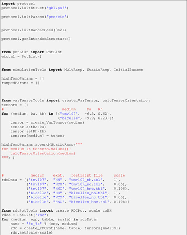
Although the protein’s covalent topology and associated parameters are established at this point, atomic positions are still undefined (or “unknown” in Xplor-NIH terminology). While the structure calculation itself is still many lines away in the script, some energy terms require valid coordinates for their setup. Thus, an arbitrary extended conformation is generated with the function genExtendedStructure, from the protocol module. An arbitrary seed number initializes Xplor-NIH’s random number generator, which is used in the computation of this conformation and in subsequent molecular dynamics stages (see Note 2). These two operations are performed as follows:

Listing 3.

Important Collections

A PotList instance (from the potList module) is an ordered collection (i.e., a sequence) specialized to hold objects that represent energy terms. It behaves itself as an energy term, so that, for example, a PotList that contains several RDC terms (e.g., associated to different restraint files) evaluates to the sum of its constituent terms. Although PotList instances are used throughout the script, a particularly central one is named etotal, created to group all the energy terms that will be used in the structure calculation (i.e., it corresponds to E_total in Eq. 1):

Listing 4.

Other important collections are the regular Python lists highTempParams and rampedParams:

Listing 5.

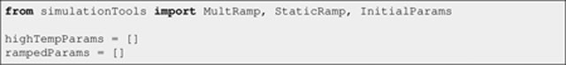
They are used to handle (i) changes in both energy scales and atomic repulsion setups (e.g., C^α-only versus all-atom interactions) between the high temperature and simulated annealing stages, and (ii) energy scale ramping within the simulated annealing stage itself. As its name suggests, objects added to highTempParams deal solely with the high temperature stage. Only instances of MultRamp or StaticRamp objects (imported here from the simulationTools module) will be added to highTempParams and rampedParams. The roles of the latter are exemplified below with the creation and configuration of the different energy terms, and should become completely clear when the structure calculation function is explained.

Energy Terms

RDC Restraints

The RDC energy term [2] requires the definition of the alignment tensor for each of the available media. The tensors dictionary, defined below, maps a user-selected medium name (the key) to the corresponding tensor object (the value). In the generation of each tensor, an estimate of its axial component D_a (Da in the Listing) and rhombicity (Rh) (e.g., as obtained from the powder pattern method [19]; see Note 3) are provided:

Listing 6.

Each molecular alignment tensor is represented by seven pseudoatoms, which describe the orientation, D_a, and the rhombicity. These pseudoatoms do not contact the protein (i.e., they are “van der Waals-invisible”), are generated automatically, and, thus, can be almost ignored. They are, however, present at the end of each output coordinate file, and can be helpful to understand and communicate the nature of the alignment, for instance, by visualizing the tensor orientation relative to the structure.

Next, a StaticRamp instance is added to highTempParams, instructing the function calcTensorOrientation (from the varTensorTools module) to optimize the orientation of each alignment tensor prior to the high temperature stage:

Listing 7.

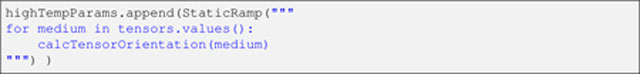
The “static” in StaticRamp’s name refers to the fact that the snippet of code used in its instantiation (i.e., the for loop) will be run as is (as opposed to a MultRamp instance). This will become obvious below.

Next, the list rdcData is created, packed with the information associated with each input RDC restraint file (see Table 1). Each item within this list is a tuple that contains the following information (in this order): the medium’s name, an arbitrary user-selected experiment name (e.g., ‘NH’ for N–H^N RDCs), the path name of the restraint file, and a relative scale factor.

Listing 8.

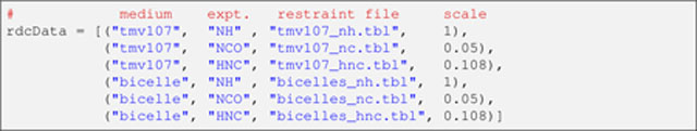
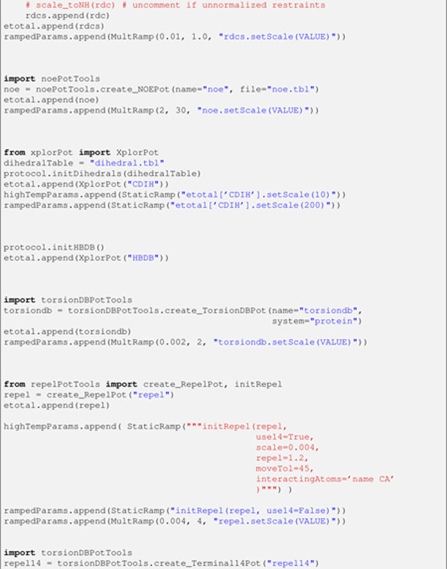
The medium’s name is used to identify the corresponding alignment tensor (i.e., it must be one of those in Listing 6). In this example, the RDCs in the restraint files have been normalized relative to the N–H^N spin pair, which increases the apparent magnitudes of the less sensitive (therefore, more error prone) non-N–H^N RDCs. So that the latter do not dominate the calculation, their respective contribution to the RDC energy term will be scaled down by the square of the inverse of the normalization factor. These relative scale constants are specified in the right-most column in Listing 8. (To use unnormalized RDCs in an Xplor-NIH calculation see Note 4.)

The RDC energy term itself is created next, by looping through each item in rdcData, and creating an individual energy term associated with the data therein:

Listing 9.

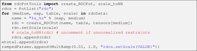
Specifically, for each loop iteration, a name is generated by combining the experiment and medium names (useful for reporting statistics later on), in turn, used in the creation of an RDC energy object. The iteration is concluded by setting the energy term’s relative scale and adding the term to rdcs (a PotList). At loop exit, rdcs involves the entire RDC dataset and, thus, represents the complete RDC energy term (i.e., E_RDC in Eq. 2), which is added to etotal. Appended to rampedParams is a MultRamp instance, which defines a range of values (from 0.01 to 1.0) for the overall RDC energy scale (w_RDC in Eq. 2). Throughout the high temperature stage, the energy scale will be given its “initial” value of 0.01 (i.e., the range’s minimum), whereas during the simulated annealing stage, it will be geometrically increased from this minimum to the maximum value of 1.0.

Distance Restraints

The NOE energy term is used to implement distance restraints (E_dist in Eq. 2). As opposed to the RDC term above, no loop is required to set up the NOE term, because all GB1 distance restraints are encapsulated in a single file:

Listing 10.

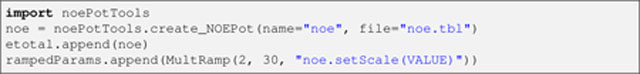
With this caveat, the setup is very similar to that of the RDC term. The energy object is created by giving it a user-selected name and the path name of the restraint file. After being added to etotal, the term is further configured within rampedParams for energy scale handling, as explained above with the RDC term.

Torsion Angle Restraints

Xplor-NIH inherits facilities from the older XPLOR program on which it is based. With continued development of Xplor-NIH, older XPLOR facilities have been deprecated in favor of rewritten versions, such as the RDC and NOE energy terms discussed above (see Note 5). The legacy XPLOR energy terms, however, can still be accessed from Xplor-NIH Python scripts (via the xplorPot module), which is useful for terms that have no native counterpart in the Python interface. This is the case of the torsion angle restraint term (E_torsion in Eq. 2) (and other terms below):

Listing 11.

To facilitate reuse of the restraint file’s path name (also required below), it is assigned to a variable (dihedralTable). The call to the protocol.initDihedrals function sets up the term, which is added to etotal as indicated. As opposed to the RDC and NOE terms above, where the energy scale is set to be uniform throughout the high temperature stage and ramped during the simulated annealing stage, here, it is configured to hold (different) uniform values in both stages. This is achieved by invoking the highTempParams list, to which a StaticRamp object is appended, specifying the constant value (of 10.0) for the high temperature stage. Similarly, the StaticRamp instance added to rampedParams specifies the energy scale value (to 200) for the entire annealing stage.

Knowledge-Based Energy Terms

With all the energy terms associated with experimental data, E_expt (Eq. 2), already configured, the first term in E_prior (Eq. 3) that we encounter is the knowledge-based hydrogen bond term E_hbdb (from Eq. 4) [17]:

Listing 12.

Since the overall energy scale of this term remains uniform throughout the entire protocol (i.e., w_hbdb in Eq. 4 is always one), there is no need for entries in highTempParams and/or rampedParams. The term is added to etotal as usual.

Next, the knowledge-based torsion angle energy term, torsionDB (E_torsionDB in Eq. 4) [18], is configured:

Listing 13.

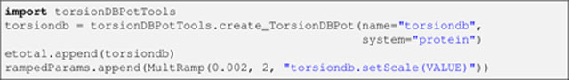
The similarities with the NOE energy term setup (Listing 10 above) are obvious. It is noteworthy that, since there is a version of this term for RNA [20], the system argument is used to choose the correct application upon the term’s creation (i.e., “protein” for GB1).

Atomic Repulsions

The generation of the atomic repulsion energy term, and its addition to etotal is performed as follows:

Listing 14.

The behavior of this term throughout the structure calculation protocol is among the most complicated, as it not only involves changes in its energy scale (exemplified with previously discussed terms) but also in the atomic interactions that are active. During the high temperature stage, only repulsions between “inflated” C^α atoms are wanted in order to promote efficient conformational sampling. Since this configuration will not change throughout that stage, it is specified with a StaticRamp instance, correspondingly added to highTempParams:

Listing 15.

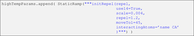
Here, noteworthy arguments to the initRepel function are use14, repel, and interactingAtoms, respectively specifying the use of 1–4 interactions (i.e., between atoms separated by three bonds), van der Waals radii (stored in the parameter file) enlarged by a factor of 1.2, and C^α repulsions only. Note that throughout the text, it is implied that interactions of (i) order lower than 1–4 are never active, and (ii) order higher than 1–4 are always active.

During the simulated annealing stage, it is required for all atoms, exhibiting realistic radii, to repel each other (excluding 1–4 interactions; see below for an explanation). Since this configuration remains unchanged during that stage, it is specified with a StaticRamp instance, added to rampedParams:

Listing 16.

The energy scale factor is familiarly configured (e.g., as in the RDC term):

Listing 17.

which specifies the geometrical increase during the simulated annealing stage from 0.004 to 4.

The torsionDB energy term introduced above (Listing 13) affects all the heavy-atom-based torsion angles of a protein (ϕ,ψ, χ₁,…, χ₄) [18], hence the exclusion of 1–4 repulsions within the simulated annealing stage (implied in Listing 16 above with the use14 argument). However, torsion angles of terminal, protonated groups, such as that involved in methyl rotation, are not considered by torsionDB. Thus, to prevent eclipsed conformations in such groups, the corresponding 1–4 interactions are introduced with an extra, repulsive energy term:

Listing 18.

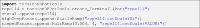
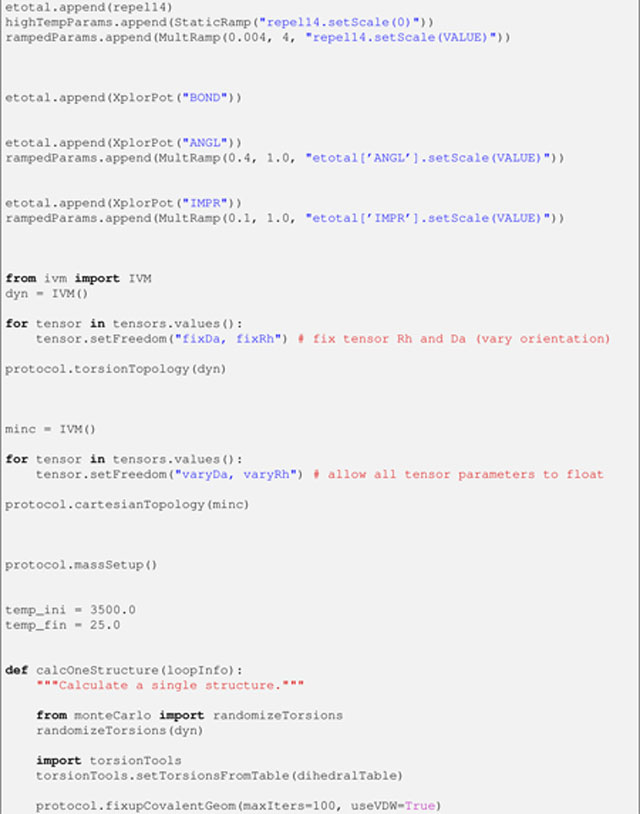
The StaticRamp instance within highTempParams nullifies the term during the high temperature stage so that only the wanted C^α repulsions are active.

The two repulsive terms just discussed embody E_repel in Eq. 3.

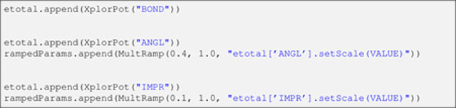
Bond Length, Bond Angle, and Improper Dihedral Energy Terms

The remaining energy terms needed to complete E_prior (Eq. 3) and E_total (Eq. 1) are those that involve bond lengths, bond angles, and improper dihedral angles (to define group chirality and planarity), which are respectively set up below without introducing any new concepts:

Listing 19.

Degrees of Freedom

Having already defined and set up all the energy terms, we focus on the configuration of the degrees of freedom used in the conformational search. This requires the introduction of IVM objects (from the ivm module, where the initials stand for Internal Variable Module [21]), which are central for performing molecular dynamics and gradient minimization. Briefly anticipating its functions, an IVM object works as follows: it is given particular degrees of freedom (e.g., torsion angle), associated to energy terms, set up according to a conformational sampling technique (e.g., for molecular dynamics: define the temperature, duration, etc.), and, finally, it is “run”, which performs the desired sampling operation. At this point in the script, however, the IVM objects are just created and assigned degrees of freedom, pending further configuration later on.

The protein evolves in torsion angle space during the entire protocol (see Note 6), except for the final Cartesian minimization stage. Thus, two IVM instances are created, starting with that configured for torsion angle space:

Listing 20.

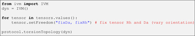
where dyn is the IVM object instance. An IVM object controls the degrees of freedom of all the atoms in the system. As previously described, each RDC molecular alignment tensor is represented by a set of (pseudo)atoms, whose degrees of freedom—and, consequently, the variables they represent, namely, the orientation, D_a, and rhombicity—are therefore under the purview of the IVM object. Since dyn will be used from the start of the structure calculation, when the protein conformation is far from optimal, the D_a and rhombicity of each tensor are fixed to their initial values (input in Listing 6), as allowing them to vary in an attempted optimization would likely distort them. This is achieved inside the above loop. Finally, the function protocol.torsionTopology configures the protein’s torsional setup.

The IVM instance reserved for the final Cartesian minimization stage, minc, is introduced next:

Listing 21.

Since the overall protein shape is not expected to change significantly during that stage, the D_a and rhombicity of each alignment tensor are allowed to vary in order to optimize them.

Finally, all atoms are given a uniform mass and friction coefficient:

Listing 22.

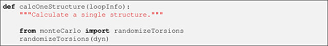
Structure Calculation

The calculation of a single structure is specified by the function calcOneStructure defined below. It relies on two useful variables, which correspond to the initial and final temperatures of the system:

Listing 23.

The initial temperature of 3500 K (temp ini variable) is that of the high temperature stage, and the starting temperature of the simulated annealing stage. The final temperature of 25 K (temp fin variable) is that at the end of the simulated annealing stage.

At this juncture, the protein atoms assume an arbitrary, extended conformation with satisfied covalent geometry, as produced by the function protocol.genExtendedStructure early on in the script (see Listing 3). The initial actions of calcOneStructure further modify the starting atomic coordinates in preparation for the high temperature stage. First, all torsion angles defined in the dyn IVM instance are randomized:

Listing 24.

Second, each torsion angle with an associated torsion angle restraint is set to the restraint’s target value:

Listing 25.

[Here is where the dihedralTable variable, assigned to the restraint file path name in Listing 11 above, becomes useful.] Finally, it is ensured that the covalent geometry is satisfied:

Listing 26.

The reason to start with the correct covalent geometry is that it cannot be improved in the calculations that take place in torsion angle space (i.e., all but the final Cartesian minimization) (see Note 6). It is also noteworthy that while the function protocol.fixupCovalentGeom silently performs molecular dynamics and minimization using the covalent energy terms and atomic repulsions, the latter (triggered by the useVDW argument) are only enabled sporadically, not necessarily enough to remove atomic clashes. Indeed, the purpose of this function (as well as protocol.genExtendedStructure) is on correcting the covalent geometry and not atomic contacts. This is certainly not an issue because the generated structure is intended to go through the high temperature molecular dynamics stage, where atomic repulsions are also limited.

Before the start of the high temperature stage, the appropriate energy scale values and atomic repulsive interactions have to be established. This is achieved in the following two lines, which clearly reveal the inner workings of lists highTempParams and rampedParams:

Listing 27.

The InitialParams function (discussed for the first time here, but originally imported from the simulationTools module in Listing 5 above) invokes the code snippet specified in each MultRamp or StaticRamp instance provided to it in an input list (here, highTempParams or rampedParams); in the case of a MultRamp instance, it does so with the first value in the associated range. The above Listing performs InitialParams(highTempParams) after InitialParams(rampedParams). The effect is to override settings of a common parameter in rampedParams by those in highTempParams. For example, InitialParams(rampedParams) configures repulsive interactions between all atom types, which is immediately reconfigured to the C^α-only mode by InitialParams(highTempParams), as desired for the high temperature stage. By contrast, InitialParams(rampedParams) sets the RDC energy scale to the initial value of the corresponding MultRamp instance, a setting that persists because it is not involved in highTempParams.

The stage is now set to configure the IVM object for torsion angle molecular dynamics. The object dyn has already been set up for torsion angle degrees of freedom (see Listing 20 above); it remains for the molecular dynamics details to be specified:

Listing 28.

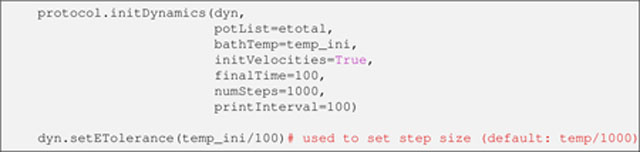
Here, with help from the function protocol.initDynamics, the input dyn is associated with the energy terms in etotal (via the potList argument), the initial temperature (via the bathTemp argument), and a dynamics duration (whichever is reached first: 100 ps, as specified by the finalTime argument, or 1000 molecular dynamics steps, as specified by the numSteps argument). In addition, it is directed that the initial atomic velocities be randomized (via the initVelocities argument) to values consistent with the temperature value. The printInterval argument specifies that every 100 steps of molecular dynamics a report is printed in the output log file, which details the energy values of each term in etotal, the kinetic energy, size of the molecular dynamics step and the current time.

An IVM objects’ eTolerance value (set on the above Listing’s last line) controls the level of energy conservation to follow when determining the time step size [21]. During high temperature dynamics this value is increased from its default of T/1000 (where T is the temperature) so that conformational space is more widely sampled.

Finally, the IVM object is run, thus performing the molecular dynamics task for which it has been configured:

Listing 29.

Since the subsequent simulated annealing stage also relies on torsion angle molecular dynamics, the dyn IVM object can be repurposed. Here, however, the temperature will be lowered in discrete steps, and dyn run for each one of them. With this in mind, dyn’s configuration follows:

Listing 30.

The configuration is similar to that previously performed (see Listing 28 above), except that (i) atomic velocities are taken from the end of the previous molecular dynamics stage (the default behavior of the initVelocities argument, implied by its absence), (ii) the energy terms are inherited from the previous configuration (etotal) and, therefore, the potList argument is left unspecified, and (iii) temperature is not specified, in anticipation of its variability within the annealing schedule. The latter is set up and run via a newly introduced object:

Listing 31.

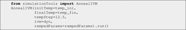
where the dyn IVM instance is provided (via the ivm argument), and the initial and final temperatures are specified (via the initTemp and finalTemp arguments, respectively), along with the temperature step (via the tempStep argument). That is, dyn is run with its latest setup (in Listing 30 above) for each of the (3500–25)/12.5 values of temperature. The rampedParams list is provided (via the rampedParams argument). For a MultRamp instance in rampedParams, the corresponding code snippet is invoked at the beginning of each step (i.e., before dyn is run), with the involved value geometrically increased in a stepwise fashion using the associated range; this is the case of energy scales such as, for example, that of the RDC term, which geometrically increases from 0.01 to 1.0 throughout the annealing schedule. For a StaticRamp instance in rampedParams, the corresponding code snippet is simply invoked as it is at the beginning of each step; this is the case of the torsion angle restraints’ energy scale, which remains at a constant value of 200, as well as the configuration of atomic repulsions (except for their energy scaling).

Gradient minimization in torsion angle space follows, not surprisingly relying on the dyn IVM object, which is configured for the Powell algorithm and run:

Listing 32.

Gradient minimization in Cartesian space is the final action of the calcOneStructure function. It relies on the IVM instance minc, already configured with Cartesian degrees of freedom (in Listing 21 above) for this purpose. The same function protocol.initMinimize above can be used to set up minc for Powell minimization, which is subsequently run:

Listing 33.

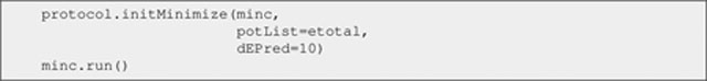
Unlike dyn, minc was not assigned the applicable energy terms (etotal) prior to minimization, hence the need to do it here (via the potList argument). The dEPred argument provides the Powell conjugate gradient algorithm [22] an estimate of the expected drop in the energy. It has been found that specifying a value of 10 for Cartesian minimization results in better optimization (the value would otherwise be 10⁻³).

Structure Gathering

At this point, the end of indentation in the script lines signifies that the calcOneStructure function definition is finished. It remains to run calcOneStructure N times, and generate statistics on the resulting structures, a task conveniently handled by a StructureLoop object (from the simulationTools module), which is setup and run as follows:

Listing 34.

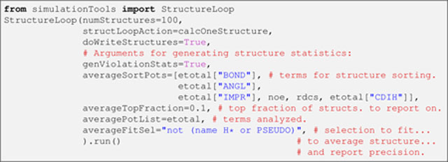
In this instantiation two kinds of arguments are noted, related to either the structure calculation or the subsequent structural analysis. numStructures, structLoopAction, and doWriteStructures belong to the former type, and respectively specify the total number of structures (N), the function used in the calculation of each of them (i.e., calcOneStructure), and whether the corresponding coordinate files (in PDB format) will be written. Each coordinate file is accompanied by an analysis file with the same name, except that the .viols extension is appended. This file contains information for each term in argument averagePotList (typically, all the terms used in the structure calculation, i.e., etotal), including detailed information about violations in each term, atomic clashes, etc. The more global structural analysis is triggered by the genViolationStats argument, and is based on the top fraction of structures specified by averageTopFraction, after all structures have been sorted from low to high energy using the terms in averageSortPots. The results of the analysis are stored in a file with the .stats extension, which reports on all the energy terms specified in averagePotList. The .stats file contains averages of fit metrics for each energy term, and a list of the most violated restraints for each energy term. averagePotList is also used to compute a regularized average structure to which the analyzed structures are fit (using the selection string given in the argument averageFitSel) to report the coordinate precision. Although not exercised here, the average structure can be written out by specifying the extra argument averageFilename to StructureLoop. StructureLoop transparently handles simultaneous parallel calculation of multiple structures either on a local computer with multiple cores, or on a cluster of computers. It is noteworthy that, after the initial folding, as done here with GB1, structures are usually refined by running a similar script (see Note 7 for details).

4. Notes

1. The PSF file of a standard protein, such as GB1, can be generated directly from the command line, by using one of the helper programs provided with Xplor-NIH (within the bin directory of Xplor-NIH’s distribution package). Assuming GB1’s amino acid sequence is stored in the file gb1.seq (see Subheading 2.2 for more details), the PSF, gb1.psf, is generated simply by typing:

   seq2psf gb1.seq
   

   The command automatically recognizes the system type (in this case, protein), and uses the corresponding default topology file (i.e., the latest version). Alternatively, when a PDB coordinate file is available (e.g., representing a conformation different from that under study), it can be similarly used to generate the PSF with the helper program pdb2psf. Additional examples of PSF generation, including less standard cases, can be found in Xplor-NIH’s distribution package, within the directory eginput/PSF generation.

2. Use of the same seed number on the same computer yields the same results.

3. Initial values for the alignment tensor D_a and rhombicity can be obtained using a maximum likelihood approach [19] which is implemented in the Xplor-NIH helper program calcDaRh. For example, based on the RDCs measured in bicelle media for GB1, this program can be run from the command line by typing:

   calcDaRh -normtype none bicelles_nh.tbl bicelles_hnc.tbl bicelles_nc.tbl
   

   The -help option of the calcDaRh command can be invoked for more details.

4. It is frequently simpler to use unnormalized RDCs. In such case, the relative energy scales in Listing 8 should be set to one, and the scale toNH line in Listing 9 should be uncommented. Additionally, the Xplor-NIH convention is for the gyromagnetic ratio of ¹⁵N to be effectively treated as positive, when it is in fact negative. If the RDC restraints have not been prepared using the Xplor-NIH convention, the function correctGyromagneticSigns (from the rdcPotTools module) should be called before create RDCPot in Listing 9.

5. Care has been taken to ensure that restraint formats supported by the old XPLOR program [3] are compatible in the newer Xplor-NIH [1, 2].

6. It is tempting (and erroneous) to think that when an IVM object (i.e., an instance of ivm.IVM) is configured with torsion angle degrees of freedom, as is the case with dyn in the main text (see Listing 20 above), there is no need to include covalent energy terms (i.e., for bond lengths and angles, and improper dihedral angles) in molecular dynamics or minimization. Indeed, while a great part of the covalent geometry remains unchanged in torsion angle space, making such energy terms unnecessary, some functional groups, however, require them. This is the case for conformationally flexible rings, such as that of proline residues, which require one endocyclic bond to behave as a spring (as restrained by the bond energy term) instead of being rigid. (Note that bond angles and improper dihedral angles involving the atoms in the mentioned bond also need to be restrained by the corresponding terms.) In addition, the default torsion angle configuration of an IVM object (applied to dyn via the protocol.torsionTopology function in Listing 20) allows flexibility in the peptide ω angle, increasing the reliance on covalent energy terms (this behavior is controlled by the optional fixedOmega argument of the above function).

7. A script for refinement of a reasonable starting structure is quite similar to fold.py presented above. The per-Listing differences are enumerated here:

   1. The call to protocol.genExtendedStructure in Listing 3 should be replaced by protocol.initCoords (′file.pdb′), where file.pdb is an input structure file to be refined.
   2. The call to calcTensorOrientation in Listing 7 should be replaced with a call to function calcTensor, after importing it from the varTensorTools module. This function computes the D_a, rhombicity, and orientation of an input alignment tensor object via singular value decomposition [23]. This full calculation (as opposed to just the orientation with calcTensorOrientation) is possible in the refinement case because a reasonable starting structure is available at the beginning of the calculation.
   3. The initial temperature (temp_ini in Listing 23) should be lowered to 3000 K.
   4. The calls to randomizeTorsions in Listing 24 and to setTorsions in Listing 25 should be removed.
   5. Finally, if one desires to refine more than one structure, a glob wildcard expression can be specified by adding the pdbFilesIn argument of StructureLoop in Listing 34 (e.g., pdbFilesIn=′fold_*.best′ would refine all the structures whose file names match the pattern fold_*.best).
      A refinement script is included in the eginput/protein directory within the Xplor-NIH distribution (as of version 2.45).

Supplemental Listing

File fold.py (a commented version can be found in the eginput/protein directory within the Xplor-NIH distribution, starting with version 2.45):

References

- 1.Schwieters CD, Kuszewski JJ, Tjandra N and Clore GM (2003) The Xplor-NIH NMR molecular structure determination package. J Magn Reson 160:66–74 [DOI] [PubMed] [Google Scholar]
- 2.Schwieters CD, Kuszewski JJ, and Clore GM (2006) Using Xplor-NIH for NMR molecular structure determination. Progr Nucl Magn Reson Spectrosc 48:47–62 [DOI] [PubMed] [Google Scholar]
- 3.Brünger AT (1993) XPLOR Manual Version 3.1. Yale University Press, New Haven: http://xplor.csb.yale.edu/xplor-info/ [Google Scholar]
- 4.Huang J-r and Grzesiek S (2010) Ensemble calculations of unstructured proteins constrained by RDC and PRE data: a case study of urea-denatured ubiquitin. J Am Chem Soc 132:694–705 [DOI] [PubMed] [Google Scholar]
- 5.Iwahara J, Schwieters CD and Clore GM (2004) Ensemble approach for NMR structure refinement against 1H paramagnetic relaxation enhancement data arising from a flexible paramagnetic group attached to a macromolecule. J Am Chem Soc 126:5879–5896 [DOI] [PubMed] [Google Scholar]
- 6.Schwieters CD and Clore GM (2014) Using small angle solution scattering data in Xplor-NIH structure calculations. Progr Nucl Magn Reson Spectrosc 80:1–11 [DOI] [PMC free article] [PubMed] [Google Scholar]
- 7.Gong Z, Schwieters CD, Tang C (2015) Conjoined use of EM and NMR in RNA structure refinement. Plos One 10:e0120445. [DOI] [PMC free article] [PubMed] [Google Scholar]
- 8.Clore GM and Schwieters CD (2004) How much backbone motion in ubiquitin is required to account for dipolar coupling data measured in multiple alignment media as assessed by independent cross-validation. J Am Chem Soc 126:2923–2938 [DOI] [PubMed] [Google Scholar]
- 9.Kuszewski J, Gronenborn AM, Clore GM (1999) Improving the packing and accuracy of NMR structures with a pseudopotential for the radius of gyration. J Am Chem Soc 121:2337–2338 [Google Scholar]
- 10. https://www.virtualbox.org.
- 11. https://www.vmware.com/products/workstation.
- 12. http://qemu.org/
- 13. http://python.org.
- 14.Shen Y and Bax A (2013) Protein backbone and sidechain torsion angles predicted from NMR chemical shifts using artificial neural networks. J Biomol NMR 56:227–241 [DOI] [PMC free article] [PubMed] [Google Scholar]
- 15.Tian Y, Schwieters CD, Opella SJ, and Marassi FM(2014) A practical implicit solvent potential for NMR structure calculation. J Magn Res 243:54–64 [DOI] [PMC free article] [PubMed] [Google Scholar]
- 16.Nilges M, Clore GM and Gronenborn AM (1988) Determination of three-dimensional structures of proteins from interproton distance data by hybrid distance geometry-dynamical simulated annealing calculations. FEBS Lett 229:317–324 [DOI] [PubMed] [Google Scholar]
- 17.Grishaev A and Bax A (2004) An empirical backbone-backbone potential in proteins and its application to NMR structure refinement and validation. J Am Chem Soc 126:7281–7292 [DOI] [PubMed] [Google Scholar]
- 18.Bermejo GA, Clore GM, and Schwieters CD (2012) Smooth statistical torsion angle potential derived from a large conformational database via adaptive kernel density estimation improves the quality of NMR protein structures. Protein Sci 21:1824–1836 [DOI] [PMC free article] [PubMed] [Google Scholar]
- 19.Warren JJ and Moore PB (2001) A maximum likelihood method for determining and R for sets of dipolar coupling data. J Magn Reson 149:271–275 [DOI] [PubMed] [Google Scholar]
- 20.Bermejo GA, Clore GM, and Schwieters CD (2016) Improving NMR structures of RNA. Structure 24:806–815 [DOI] [PMC free article] [PubMed] [Google Scholar]
- 21.Schwieters CD, and Clore GM (2001) Internal coordinates for molecular dynamics and minimization in structure determination and refinement. J Magn Reson 152:288–302 [DOI] [PubMed] [Google Scholar]
- 22.Powell MJD (1977) Restart procedures for the conjugate gradient method. Math Program 12:241–254 [Google Scholar]
- 23.Losonczi JA, Andrec M, Fischer MW, and Prestegard JH (1999) Order matrix analysis of residual dipolar couplings using singular value decomposition. J Magn Reson 138:334–342 [DOI] [PubMed] [Google Scholar]