Assessment of heterogeneity in an individual participant data meta‐analysis of prediction models: An overview and illustration

Abstract

Clinical prediction models aim to provide estimates of absolute risk for a diagnostic or prognostic endpoint. Such models may be derived from data from various studies in the context of a meta‐analysis. We describe and propose approaches for assessing heterogeneity in predictor effects and predictions arising from models based on data from different sources. These methods are illustrated in a case study with patients suffering from traumatic brain injury, where we aim to predict 6‐month mortality based on individual patient data using meta‐analytic techniques (15 studies, n = 11 022 patients). The insights into various aspects of heterogeneity are important to develop better models and understand problems with the transportability of absolute risk predictions.

1. INTRODUCTION

Clinical prediction models aim to provide estimates of absolute risk of an endpoint. Common endpoints are the presence of a disease (establishing a diagnosis according to a reference standard) and the occurrence of a future event (prognosis, eg, mortality within 30 days, within 6 months, or longer follow‐up).1 Prediction models are increasingly common in the medical literature, and multiple models may be available for the same type of patients for similar endpoints.2 Published prediction models often use different predictors to derive predictions for individual patients.3 Moreover, many prediction models are developed in relatively small samples from a specific setting, eg, a single hospital.4

Prediction models that are developed from small samples are prone to statistical overfitting, and may therefore have poor accuracy when applied to new patients.5 Applying penalization or shrinkage techniques may limit such problems,6, 7 but better prediction models can be derived with larger numbers of patients. If these larger numbers of individual patient data (IPD) come from different sources, we may aim to develop a global prediction model, with improved validity across multiple settings or populations. A global model can, for instance, be derived by merging all IPD sets and estimating a common baseline risk and set of predictor effects. This strategy clearly obfuscates possible differences between studies and ignores clustering of patients within studies. Several more advanced strategies have recently been proposed. Access to data on large numbers of patients from different settings allows us to assess between setting heterogeneity, following principles from meta‐analysis (MA).8, 9 10, 11

In the current paper, we aim to describe and propose approaches for assessing heterogeneity in predictor effects and predictions arising from prediction models based on data from different studies. We consider between‐study heterogeneity with respect to missing values, covariate and endpoint distribution, and model performance. Such assessment of heterogeneity may serve two purposes:

• (1) to support or refute the idea of a global prediction model;
• (2) to appropriately indicate the uncertainty when applying the global model across different populations.

This paper starts with an overview of some key characteristics of commonly used regression models to estimate absolute risk, and some background on a case study where we develop a global model based on IPD from 15 studies to predict 6‐month mortality after traumatic brain injury (TBI).12 Section 3 considers characteristics of the included studies and differences in study design and included patients and differences in case‐mix, while Section 4 focuses on dealing with missing values. Heterogeneity in predictor effects and predictions is discussed in Sections 5 and 6.

Section 7 is a general discussion, where we not only consider the situation of having access to IPD from each study but also variants such as having access to only one IPD data set, or no IPD at all. We end with some reflections on the impact of heterogeneity on model performance and model applicability.

2. PREDICTION MODELS AND MA

2.1. Common types of regression models

The most common prediction problems in medicine concern binary endpoints, where logistic regression models are often used to estimate the probability that a certain endpoint Y is present or will occur conditional on the 1 × p row vector of predictors X , where p is the number of predictors, ie, $P\left(Y=1|\mathit{X}=\mathit{x}\right)=\frac{\exp \left(\alpha +\mathit{X}{\mathit{\beta }}^{\prime }\right)}{1+\exp \left(\alpha +\mathit{X}{\mathit{\beta }}^{\prime }\right)}.$

Here, α is the model intercept, and β represents a row vector reflecting the relative effects of the predictor values X. We refer to Xβ′ as the linear predictor or prognostic index, which summarizes the effects of the predictors X.5 The intercept α is kept separate from the linear predictor. In terms of odds of the endpoint, we can also write

$$\text{Odds}\left(Y=1|\mathit{X}=\mathit{x}\right)=\text{exp}\left(\alpha \right)\text{exp}\left(\mathit{X}{\mathbf{\beta }}^{\prime }\right).$$

For time‐to‐event endpoints, such as survival, the baseline risk is dependent on time and can therefore no longer by summarized by a single constant. For this reason, time‐to‐event endpoints are commonly modeled with Cox regression

$$h\left(t|\mathit{x}\right)=h_0\left(t\right)\text{exp}\left(\mathit{X}{\mathbf{\beta }}^{\prime }\right).$$

We notice that the logistic regression model contains a constant α, while the Cox model contains a nonparametric baseline hazard h ₀(t) that plays the role of a generalized constant. Both reflect the baseline risk in a prediction model. We can make the baseline risk more interpretable by subtracting the mean value for the predictors X, as is common for the Cox regression model. Moreover, we might smooth the baseline hazard to facilitate calculation of absolute risks.13

Here, we focus on IPD‐MA using logistic regression models. Extensions of these methods to Cox regression models are discussed in Appendix A, along with situations where one IPD is available and where no IPD is available.

2.2. Meta‐analysis for prediction

Similar to the MA of randomized trials, it is readily possible to summarize parameter estimates from multiple studies by calculating a weighted average for the intercept term and regression coefficients.14 Issues of interest are summary estimates of baseline risk and predictor effects, as well as corresponding estimates of between‐study heterogeneity. Even more important is the heterogeneity in the linear predictor and absolute risk predictions. These predictions depend on the joint effects of all predictors and baseline risk and need to be reasonably similar across studies for a prediction model to be labeled “generalizable.” We hence focus on three aspects of heterogeneity for predictions, namely, in baseline risk, predictor effects, and the linear predictor (which is directly linked to absolute risk predictions).

2.3. Case study

For illustrative purposes, we analyze 15 studies of patients suffering from TBI, including IPD from 11 randomized controlled trials and four observational studies. These studies were part of the IMPACT project, where a total of 25 prognostic factors were considered for prediction of 6‐month mortality.15 Mortality occurred in 20% to 40% of the patients, while follow‐up was nearly complete for the 6‐months status (Table 1). Three different models were developed of increasing complexity.12 The core model used three key predictors, ie, age, the assessment of Glasgow Coma Scale motor score at admission, and pupillary reactivity at admission. The CT model contained the predictors of the core model, secondary insults (hypoxia and hypotension) and results from a CT scan (Marshall CT classification system, traumatic subarachnoid hemorrhage and epidural hematoma). The most elaborate model contained the predictors of the CT model and results from lab tests (glucose and hemoglobin levels).12 For our case study, we focus on the global CT model. This model was fitted with study as a main effect, and common effects for the predictors. R code to perform the analyses is available from the authors (R version 3.5.0, The R Project for Statistical Computing). The data that support the findings of this study are available from the corresponding author upon reasonable request.

Table 1.

Description of 15 IMPACT data sets of 11 022 patients with traumatic brain injury (TBI)

Nr.	Name	Enrollment period	Type1	n
1	TINT	1991–1994	RCT	1118
2	TIUS	1991–1994	RCT	1041
3	SLIN	1994–1996	RCT	409
4	SAP	1995–1997	RCT	919
5	PEG	1993–1995	RCT	1510
6	HIT I	1987–1989	RCT	350
7	UK4	1986–1988	OBS	791
8	TCDB	1984–1987	OBS	603
9	SKB	1996–1996	RCT	126
10	EBIC	1995–1995	OBS	822
11	HIT II	1989–1991	RCT	819
12	NABIS	1994–1998	RCT	385
13	CSTAT	1996–1997	RCT	517
14	PHARMOS	2001–2004	RCT	856
15	APOE	1996–1999	OBS	756

¹ Type of study, RCT: randomized controlled trial, OBS: observational cohort

3. STUDY CHARACTERISTICS

3.1. Heterogeneity in study design

Meta‐analysis requires a reasonable degree of similarity between studies to provide meaningful summary estimates. It is therefore important to consider whether the included studies have major differences in their design, selection of subjects, and setting, as this may affect the baseline risk and/or predictor‐endpoint relations. For the 15 TBI studies, four were performed in relatively unselected populations (“surveys,” observational cohorts), with broad inclusion criteria. Inclusion criteria were stricter for 11 randomized controlled trials. The studies also varied in the calendar time of enrollment of patients, and one study was rather small (#9, SKB, Table 1).

3.2. Heterogeneity in case‐mix

Between‐study heterogeneity in case‐mix is a common source of heterogeneity in baseline risk and predictor‐endpoint associations. Briefly, heterogeneity in case‐mix occurs when the distribution of patient characteristics varies across studies. In the TBI case study, there appear to be systematic differences between observational studies and RCTs in terms of observed mortality and patient characteristics (ie, the case‐mix distribution) (Table 2). Case‐mix variability was particularly high in the 4 observational studies, which we quantified by the standard deviation of the linear predictor of the global model fitted using all studies. We might also quantify this heterogeneity by study‐specific models, but the standard deviation of the linear predictor would then depend on both case‐mix and estimated coefficients.

Table 2.

Six‐month mortality, case‐mix distribution, and discriminative ability of the membership model in identifying membership of a specific study

Nr.	Name	6‐month mortality	Mean lp	SD lp	Membership c‐statistic
1	TINT	25%	−1.42	1.23	0.62
2	TIUS	22%	−1.6	1.13	0.65
3	SLIN	23%	−1.42	0.99	0.76
4	SAP	23%	−1.44	1.02	0.60
5	PEG	24%	−1.51	1.26	0.67
6	HIT I	28%	−1.23	1.35	0.68
7	UK4	45%	−0.27	1.77	0.64
8	TCDB	44%	−0.36	1.74	0.67
9	SKB	27%	−1.19	0.99	0.75
10	EBIC	34%	−0.98	1.81	0.63
11	HIT II	23%	−1.49	1.10	0.63
12	NABIS	26%	−1.27	1.08	0.65
13	CSTAT	22%	−1.57	1.16	0.61
14	PHARMOS	17%	−1.78	0.79	0.68
15	APOE	15%	−2.45	1.65	0.73

lp: linear predictor, based on a common prediction model and study‐specific predictor values; membership c statistic: discriminative ability to separate a specific study from all other studies, where a high c‐statistic reflects substantial differences in baseline characteristics and outcome.

In the TBI case study, we further note substantial differences in the incidence of the end point (6‐month mortality): 17% in the most recent trial (study #14) versus 42% in a survey (study #7). The difference in mortality rate may partly be explained by study design, since RCTs only included patients who survived long enough to be included in the trial, while the observational studies also included patients who died shortly after arriving at a hospital.

It is also possible to inspect the distributions of individual predictors. These are rather different between studies (Figure 1). We note that this inspection does not take into account the possible correlation between predictors.

Figure 1.

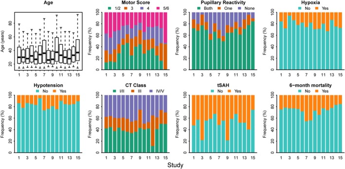
Distribution of patient characteristics in 15 studies with 11 022 traumatic brain injury patients, after single imputation of missing values [Colour figure can be viewed at wileyonlinelibrary.com]

Finally, a summary measure of case‐mix similarity between studies can be obtained using a membership model, where we quantify how well we can separate patients from different studies from each other (using the c‐statistic).16 We therefore developed a membership model using multinomial logistic regression (Table 2), where study membership was the outcome. We included all predictor variables of the CT model and 6‐month mortality as covariates. A variant of this membership model might include only predictor variables. The c‐statistic of the membership model can be calculated by comparing the predicted probabilities for patients from one study with the predicted probabilities of patients not included in that study. We found that studies 3, 9, and 15 were somewhat different from the other studies, with c‐statistics above 0.70, based on the distribution of patient characteristics and mortality.

4. MISSING PREDICTOR VALUES AND MA

4.1. Missing values and imputation

Imputation of missing values poses specific challenges in the context of development or validation of a global prediction model. Advanced imputation approaches may be required to fully address between‐study heterogeneity in the correlation structure between predictors and endpoint. Ignoring such heterogeneity in the imputation procedure may lead to bias in the estimated coefficients and their associated standard errors, to bias in estimates of between‐study heterogeneity, and to model validation results that are too optimistic.11, 17

More advanced multilevel imputation methods have recently proposed to impute missing values in large, clustered data sets such as IPD‐MA and can also be used to impute covariates that are systematically missing for one or more studies.18, 19, 20, 21, 22, 23 In our case study, we applied the simpler approach as used previously by Steyerberg et al,12 where the authors imputed missing predictors using the study as a fixed effect in the imputation model. This imputation model admittedly only adjusts for heterogeneity in the levels and prevalence of missing predictors.

5. HETEROGENEITY IN COMBINATIONS OF PREDICTOR EFFECTS

5.1. Estimating stratified predictor effects

After considering general between‐study heterogeneity and imputing missing values, an important step is to estimate predictor‐endpoint associations across the available data sets. Ideally, the global prediction model is prespecified. Prior knowledge and/or clinical expertise may have guided the selection of predictors as well as the choice of linear or nonlinear forms in case of continuous predictors.6, 24 In practice, some form of selection may be based on predictor‐endpoint associations observed across the set of studies considered in the MA. Such a selection will cause only limited bias if sample sizes are large and the number of candidate predictors small. We first discuss full stratification by study. Subsequently, we discuss several simplifications.

The presence of heterogeneity between J studies may be considered as follows. First, we consider stratified estimation of the model intercept and regression coefficients for each study j (Table 3)

$$P\left(Y=1|\mathit{X}=\mathit{x},\text{study}j\right)=\frac{\exp \left({\alpha }_j+\mathit{X}{\mathit{\beta }}_{\mathit{j}}{}^{\prime }\right)}{1+\exp \left({\alpha }_j+\mathit{X}{\mathit{\beta }}_{\mathit{j}}{}^{\prime }\right)}.$$

Table 3.

Multivariable logistic regression models to predict mortality 6 months after traumatic brain injury fitted separately in each of the 15 studies. We show the estimated regression coefficients with associated standard errors for the 15 studies. A two‐stage multivariate meta‐analysis provided pooled estimates of the between‐study variance parameter tau and prediction intervals for the regression coefficients. The between versus within‐study heterogeneity is summarized in I ² estimates

Study	Intercept	Age	Motor score	Pupillary reactivity	Hypoxia	Hypotension	CT class	tSAH
1	−1.22 (0.09)	0.20 (0.05)	−0.39 (0.08)	0.41 (0.11)	0.36 (0.20)	1.03 (0.21)	0.56 (0.10)	1.01 (0.17)
2	−1.40 (0.10)	0.21 (0.07)	−0.40 (0.08)	0.36 (0.11)	0.46 (0.18)	0.75 (0.19)	0.34 (0.10)	0.74 (0.17)
3	−1.35 (0.22)	0.28 (0.09)	−0.28 (0.12)	0.71 (0.23)	−0.36 (0.58)	0.97 (0.35)	0.47 (0.15)	0.70 (0.37)
4	−1.34 (0.09)	0.20 (0.06)	−0.14 (0.07)	0.74 (0.11)	0.68 (0.24)	0.22 (0.23)	0.33 (0.10)	0.82 (0.18)
5	−1.73 (0.10)	0.21 (0.05)	−0.52 (0.06)	0.52 (0.08)	0.33 (0.16)	0.77 (0.17)	0.38 (0.08)	0.54 (0.14)
6	−1.41 (0.19)	0.30 (0.09)	−0.45 (0.13)	0.82 (0.17)	0.00 (0.38)	−0.60 (0.63)	0.38 (0.08)	0.95 (0.29)
7	−0.93 (0.11)	0.43 (0.05)	−0.30 (0.09)	1.01 (0.12)	0.07 (0.21)	1.21 (0.22)	0.36 (0.11)	0.70 (0.19)
8	−0.73 (0.12)	0.47 (0.07)	−0.42 (0.10)	0.57 (0.12)	0.36 (0.27)	1.31 (0.25)	0.43 (0.12)	0.63 (0.21)
9	−1.28 (0.35)	0.38 (0.16)	−0.23 (0.22)	0.34 (0.26)	−0.40 (0.54)	0.71 (0.59)	0.64 (0.28)	0.72 (0.63)
10	−1.41 (0.12)	0.40 (0.05)	−0.45 (0.09)	0.80 (0.12)	0.54 (0.23)	0.73 (0.24)	0.31 (0.11)	0.81 (0.19)
11	−1.44 (0.11)	0.22 (0.06)	−0.40 (0.09)	0.43 (0.11)	0.21 (0.23)	0.34 (0.30)	0.38 (0.11)	0.97 (0.19)
12	−1.49 (0.17)	0.24 (0.10)	−0.39 (0.11)	0.68 (0.14)	0.35 (0.28)	0.83 (0.34)	0.36 (0.21)	0.60 (0.26)
13	−1.43 (0.14)	0.22 (0.09)	−0.42 (0.11)	0.68 (0.14)	−0.04 (0.34)	0.26 (0.30)	0.52 (0.14)	0.76 (0.24)
14	−1.61 (0.11)	0.17 (0.07)	−0.34 (0.09)	0.29 (0.16)	0.06 (0.23)	0.46 (0.26)	0.53 (0.11)	0.42 (0.21)
15	−2.07 (0.18)	0.52 (0.07)	−0.59 (0.15)	0.91 (0.16)	0.33 (0.28)	0.54 (0.37)	0.29 (0.14)	0.47 (0.26)
Pooled	−1.35 (0.07)	0.28 (0.03)	−0.38 (0.03)	0.61 (0.06)	0.27 (0.07)	0.71 (0.10)	0.40 (0.03)	0.72 (0.06)
Estimated τ	0.25	0.09	0.07	0.17	0.08	0.27	0.06	0.08
95% Prediction interval	[−1.92, −0.78]	[0.08, 0.48]	[−0.55, −0.20]	[0.21, 1.01]	[0.05, 0.50]	[0.08, 1.34]	[0.25, 0.55]	[0.50, 0.93]
I 2	84%	67%	35%	65%	0%	49%	0%	2%

Age was analyzed as a continuous predictor, per 10 years; Motor score, pupillary reactivity, and CT class were analyzed as continuous predictors, coded as in Figure 1. Hypoxia, hypotension, and tSAH were binary predictors. For interpretation of the baseline risk (the intercept α), we standardized predictors by subtracting the overall means of predictor values.

For descriptive purposes, we propose forest plots for visualization of the heterogeneity in predictor effects (Figure 2). Additionally, pooled estimates with associated (approximate) prediction intervals and I ² estimates based on a multivariate MA can provide further insight in the extent of between‐study heterogeneity.14

Figure 2.

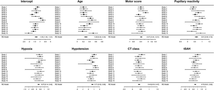
Forest plots showing estimated multivariable logistic regression coefficients and associated 95% confidence interval per study. The largest heterogeneity was noted for pupillary reactivity (τ = 0.17) and hypotension (τ = 0.27)

5.2. Pooling with full stratification

For pooled analysis, we consider ${\widehat{\mathit{\theta }}}_{\mathit{j}}=\left({\widehat{\alpha }}_j,{\widehat{\mathit{\beta }}}_j\right)$, the (P + 1)‐vector of regression coefficients with associated within‐study covariance matrix $\widehat{\mathit{S}}$ _j. More specifically, the study‐specific model is given by ${\widehat{\mathit{\theta }}}_j\mid {\mathit{\theta }}_j\sim \mathit{\text{MVN}}\left({\mathit{\theta }}_j,{\mathit{S}}_j\right).$ The distribution of θ_j over the population is assumed to be a multivariate normal distribution

$${\mathit{\theta }}_j\sim \mathit{\text{MVN}}\left(\mathit{\mu },\mathbf{T}\right).$$

To avoid identifiability problems, we assume that the number of studies exceeds the number of study‐specific parameters, ie, N _s > P + 1. Simplifications can be made by adopting an autocorrelation structure or specifying a diagonal matrix for T.

Insight in the heterogeneity of the model predictors is gained by first fitting the model for each study separately, yielding study‐specific estimates ${\widehat{\alpha }}_j\text{and}{\widehat{\mathit{\beta }}}_j$ (Table 3 and Figure 2). The IPD are needed to obtain the full within‐study covariance matrix S _j. These covariance matrices are typically not available from published studies, and are the key benefit of having access to IPD rather than published results only. The parameters of the global prediction model can be estimated from the model ${\widehat{\mathit{\theta }}}_j\sim \mathit{\text{MVN}}\left(\mathit{\mu },\mathbf{T}+{\widehat{\mathit{S}}}_j\right)$, where ${\widehat{\mathit{\theta }}}_j$ contains the study‐specific intercept term ${\widehat{\alpha }}_j$and regression coefficients ${\widehat{\mathit{\beta }}}_j$, and ${\widehat{\mathit{S}}}_j$ represents the corresponding within‐study covariance matrix. The between‐study covariance matrix of the pooled intercept term and predictor effects is given by T. Fitting this model also yields the covariance matrix ${\mathit{S}}_{\widehat{\mathit{\mu }}}$ of the estimate $\widehat{\mathit{\mu }}$ of μ. This should not be confused with covariance matrix T of the random effects.

The aforementioned approach to an IPD‐MA is a two‐stage approach because studies are first analyzed individually and corresponding results are then combined in a second multivariate step. A one‐stage approach would fit a logistic regression model with random effects. A full specification of this model for patient i in study j may be as follows:

$$\begin{array}{cc}{Y}_{\mathit{\text{ij}}}& \sim \text{Bernoulli}\left(p_{\mathit{\text{ij}}}\right),\\ \text{logit}\left(p_{\mathit{\text{ij}}}\right)& ={\alpha }_j+{\mathit{X}}_{\mathit{\text{ij}}}{\mathit{\beta }}_j{}^{\prime },\\ \left({\alpha }_j,{\mathit{\beta }}_{\mathit{j}}\right)& \sim \mathit{\text{MVN}}\left(\mathit{\mu },\mathbf{T}\right).\end{array}$$

The one‐stage approach is computationally more demanding than the two‐stage approach, and is expected to give similar results with similar model specification and reasonable sample size.8, 25 In the case study, differences between the one‐ and two‐stage pooling were negligible. We present the two‐stage results in Table 3. The between‐study variance parameter ${\tau }_{\mathit{\text{ii}}}^2$ was relatively large compared to the pooled SE for three predictors (age, pupillary reactivity, and hypotension), with relatively large prediction intervals (Table 3).

5.3. Heterogeneity in predictions from different cohorts

Predictor effects show substantial heterogeneity across cohorts (Table 3). On the other hand, the correlation between predictors within the studies may make that the resulting predicted probabilities between studies for a patient with the same characteristics are still quite close. We propose to further consider differences between predictions for all covariate patterns that occur across the studies. We hereto construct scatter plots of predicted probabilities according to models fitted in each of the individual studies (Figure 3). We label this approach a 1‐to‐1 comparison of study‐specific model predictions, since predictions from models from each study are each compared to each other. For the case study, each comparison includes the 11 022 patients in the IPD data set. We then note that some studies provide very similar predictions, eg, study 1 and 2. This fits with the fact that these are similar trials, one recruiting patients in the US and the other internationally. Other studies provide somewhat different predictions compared to the other studies, eg, studies 6, 8, 9, and 15. This is partly attributable to differences in baseline risk, reflected in lines below or above the line of identity in Figure 3.

Figure 3.

Correlation between predictions of study‐specific models in a pairwise comparison between studies: 1‐to‐1 comparisons of predictions for all patients in the individual patient data set (n = 11 022)

The effect of differences in predictor strengths on the predictions can be seen from the “veins” in the plot. For instance, when comparing the prediction based on the model developed in study 6 with the predictions made by the models developed in the other studies, the plot typically shows two lines around which the predictions are clustered. This reflects that the regression coefficient of the predictor “hypoxia” is close to zero in study 6 and is different from zero in the other studies (Table 3). In other comparisons multiple “veins” are visible, attributable to differences in predictor strength of predictors with multiple categories, such as motor score and pupillary reactivity.

5.4. Simplifications with respect to heterogeneity

Several simplifications are possible when the extent of heterogeneity across studies is limited. The strongest simplification is to ignore any heterogeneity and thus to assume that T = 0. This implies that all studies agree on the baseline risk and predictor effects in the global model, and that differences in study‐specific estimates only appear due to sampling error. This simplification will not be realistic for most applications.

A less drastic simplification is to assume that the intercepts α_s may vary between studies but that the predictor effects β_j are common.8, 9 We label this a common effect approach with respect to β_j. Several estimation procedures may be followed to account for differences in baseline risk. If the number of studies is limited, say less than 5 studies, it is usually possible to condition on the “study” variable by estimating a separate intercept for each study. Alternatively, when more studies are available, it is reasonable to assume a Normal random effects distribution for the intercept terms.14 This second approach allows for a simple summary estimate of the between‐study heterogeneity in the intercept as ${\tau }_{\alpha }^2$. The corresponding logistic regression model is specified as follows:

$$\begin{array}{cc}{Y}_{\mathit{\text{ij}}}& \sim \text{Bernoulli}\left(p_{\mathit{\text{ij}}}\right),\\ \text{logit}\left(p_{\mathit{\text{ij}}}\right)& ={\alpha }_j+{\mathit{X}}_{\mathit{\text{ij}}}\mathit{\beta }{}^{\prime },\\ {\alpha }_j& \sim N\left(\alpha ,{\tau }_{\alpha }^2\right).\end{array}$$

If ${\tau }_{\alpha }^2$ is substantial, this implies that adjustments for the intercept need to be considered when applying the global model in a local setting (see discussion). The heterogeneity between studies can well be summarized in measures such as the median odds ratio (MOR).26

The assumption of common predictor effects β_j can be weakened by specifying that the linear predictors X_ijβ_j share a common direction in covariate space, but that the size of their effects might be systematically different. This can be modeled by a rank = 1 model

$$\begin{array}{cc}{Y}_{\mathit{\text{ij}}}& \sim \text{Bernoulli}\left(p_{\mathit{\text{ij}}}\right),\\ \text{logit}\left(p_{\mathit{\text{ij}}}\right)& ={\alpha }_j+{\gamma }_j{\mathit{X}}_{\mathit{\text{ij}}}{\mathit{\beta }}^{\prime }\mathbf{,}\\ \left({\alpha }_j,{\gamma }_j\right)& \sim \mathit{\text{MVN}}\left(\left(\alpha ,1\right),\mathbf{T}\right),\end{array}$$

and hence, E[γ_sβ] = β. In this model, the random variation between studies is described by the correlated pair (α_s, γ_s). The study‐specific relative effects are then allowed to vary in a proportional way.27 Estimation of this model is possible with a nonlinear mixed effect model, such as available with proc nlmixed in SAS software. We can approximate this model by fitting a model ignoring between‐study heterogeneity on all available patients to derive a linear predictor for each patient and subsequently fitting a random effect model with random intercept α_j and a random slope γ_j for the linear predictor. Both approaches gave very similar results in our case study, and hence, we present the results from the approximation using two steps.

A further weakening of the restrictiveness is obtained by allowing models of higher rank, such as a rank = 2 model. Again, this model can be estimated with a nonlinear mixed model, and approximated in a two‐step approach with first estimating the linear predictor globally and subsequently fitting a random effect model with the linear predictors as covariates with random slopes. In these restricted models of rank 1 or rank 2, the covariance matrix T has a simpler structure compared to the fully stratified model with study‐specific predictor effects.

5.5. Heterogeneity in specific predictions of the prediction model

In the fully stratified model, the baseline risks and predictor effects show considerable variability over the studies (Table 3). The resulting predicted probabilities also show quite some variability (Figure 3). If we consider a fixed value of the covariate vector, x₀, we can compute an approximate 95% prediction interval for new studies of P(Y = 1| x₀). Since

$$\mathit{\theta }\sim \mathit{\text{MVN}}\left(\widehat{\mathit{\mu }},\mathbf{T}+{\widehat{\mathit{S}}}_{\widehat{\mathit{\mu }}}\right),$$

we can estimate this interval using

$${\text{logit}}^{-1}\left({\mathit{x}}_0\widehat{\mathit{\mu }}\pm 1.96\sqrt{{\mathit{x}}_0\left(\mathbf{T}+{\widehat{\mathit{S}}}_{\widehat{\mathit{\mu }}}\right){\mathit{x}}_0^{\prime }}\right).$$

This is an approximate approach since it ignores the uncertainty introduced by estimating the within‐ and between‐study covariance matrices. For this reason, a Student‐T, rather than a Normal distribution, is often used to calculate confidence intervals. Similarly, approximate 95% prediction intervals for new studies can be constructed for the rank = 1 model and random intercept model. By keeping all but one predictor fixed, we can then investigate the heterogeneity of predictions across different values of this predictor. The values of the other predictors need to be chosen, for example as representative values, ie, the median for continuous predictors, and the most common category for categorical predictors.

We illustrate this approach for the age effect for otherwise average risk patients in the TBI case study. Obviously, the 95% prediction interval is smallest with a naïve single fit model, where we ignore any between‐study heterogeneity. The common effect model assumes fixed effects per study but leaves the baseline risk free. The uncertainty is larger when we allow for between‐study differences in the predictor effects with a rank = 1 model or a fully stratified model (Figure 4). Note that the risk predictions according to age and their uncertainty depend on the choice of values for the other predictors in the model.

Figure 4.

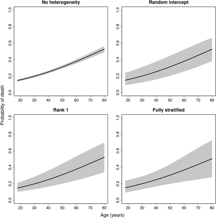
Prediction intervals for new studies assuming a fixed effects model, random intercept model, rank = 1 model, or fully stratified model

5.6. Model selection

We thus far described models that allow for different degrees of heterogeneity in predictor effects and/or baseline risk. Selecting the most appropriate model for the data at hand can be based on information criteria such as AIC/BIC or using formal statistical tests comparing the different models. We propose to apply the following test procedure. A similar type of test was recently proposed for selecting an update method for existing prediction models,28 and longer ago for selection of functional forms of covariates in fractional polynomials.29 We propose to perform a series of likelihood ratio tests which start with the fully stratified model and consider simplifications from that systematically. These tests require assessing the significance of the variance components of random effect models. Since these parameters are at the boundary of the parameter space under the null when testing if the variance is different from zero, a mixture of χ²‐distributions is required to obtain a p‐value.30 Hence, we compare the following:

1. The fully stratified model against a model without any heterogeneity (simple logistic regression ignoring any clustering of patients). The distribution used to calculate the p‐value is a 50:50 mixture of two χ²‐distributions with degrees of freedom equal to $\frac{\left(p+1\right)p}{2}$ and $\frac{p\left(p-1\right)}{2}$, where p is the number of regression coefficients included in the model; if the test is not significant, select the model without any heterogeneity; otherwise, continue.

2. The fully stratified model against a model with heterogeneity in baseline risk. Here, a 50:50 mixture of two χ²‐distributions with degrees of freedom is equal to $\frac{p\left(p-1\right)}{2}$ and $\frac{\left(p-1\right)\left(p-2\right)}{2}$; if nonsignificant, select the model with heterogeneity in baseline risk; otherwise, continue.

3. The fully stratified model against the rank = 1 model. Here, the variance components tested are not on the boundary of the parameter space; a χ²‐distribution with $\frac{\left(p+1\right)p}{2}-3$ degrees of freedom is used; if nonsignificant, select the rank = 1 model; otherwise, select the fully stratified model.

In our case study, the closed‐test procedure selects the rank = 1 model as the most appropriate model (Table 4).

Table 4.

Comparison of variants of a global model in the TBI case study with 15 studies to predict 6‐month mortality

Model variant	Baseline risk	Predictor effects	Case study	−2 log‐likelihood	p‐value of
					fully stratified
					fit against
					other model
Fully stratified	Per study	Per study	See Table 2	9750
Single fit	Common	Common	‐	9922	p < 0.0001
Common effect	Per study	Common	τα = 0.29	9810	p < 0.0001
Rank 1	Per study	Proportional per study	τα = 0.24; τγ = 0.12	9791	p = 0.16

5.7. Observed heterogeneity in predictions

When substantial heterogeneity is observed in predictions across included studies, study‐level covariates should be considered in the prediction model. These may explain heterogeneity in predictions across studies. In our case study, we considered the following study‐level covariates in the rank = 1 model, ie, year of start of study, RCT, or observational study. We found that the heterogeneity in slope could be explained partly by the whether a study was an observational study or RCT. Accounting for study type, there remained statistically significant heterogeneity in baseline risk. We hence conclude that the appropriate model for the case study would a global model, separately for observational studies and RCTs, with a random effect for study to allow for heterogeneity in baseline risk. Predictor effects for observational studies appear to be larger compared to predictor effects in RCTs (Table 5). The heterogeneity in baseline risk seems higher for observational studies, reflected in the higher standard deviation of the model intercept.

Table 5.

Logistic regression coefficients of models stratified by observational studies and RCTs

	Model based on
	Observational studies	RCT
Intercept	−1.27	−1.41
Age	0.43	0.22
Motor score	−0.42	−0.37
Pupillary reactivity	0.82	0.52
Hypoxia	0.28	0.27
Hypotension	1.03	0.62
CT class	0.34	0.42
tSAH	0.68	0.73
τα	0.44	0.14

6. VALIDATION OF MODELS DEVELOPED IN AN IPD MA

6.1. Heterogeneity in calibration of predictions

Calibration can well be assessed graphically, with some summary statistics such as calibration intercept and calibration slope.31, 32, 33, 34 A natural approach is to consider the cross‐validated performance, where models are developed for all studies minus one, for what has been labeled “internal‐external validation.”9 ^, 35 ^, 36 We leave one study out at a time, which leads to 15 validations for the case study. Here, we validate the rank=1 model, including the study‐level covariate “observational study versus RCT.” We note some miscalibration in the observational studies with higher mortality than predicted in #7 and #8, while #15 showed less mortality than predicted (Figure 5). The higher degree of miscalibration for the observational studies is in line with the larger estimated heterogeneity of the random intercept. Overall, patterns of calibration were reasonable for most trials, although a recent trial (#14) had somewhat lower than expected mortality (Figure 6).

Figure 5.

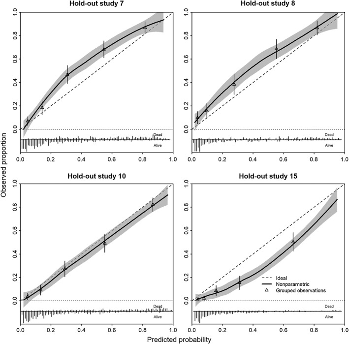
Calibration plots of model developed in observational studies in a leave‐one‐study‐out cross‐validation

Figure 6.

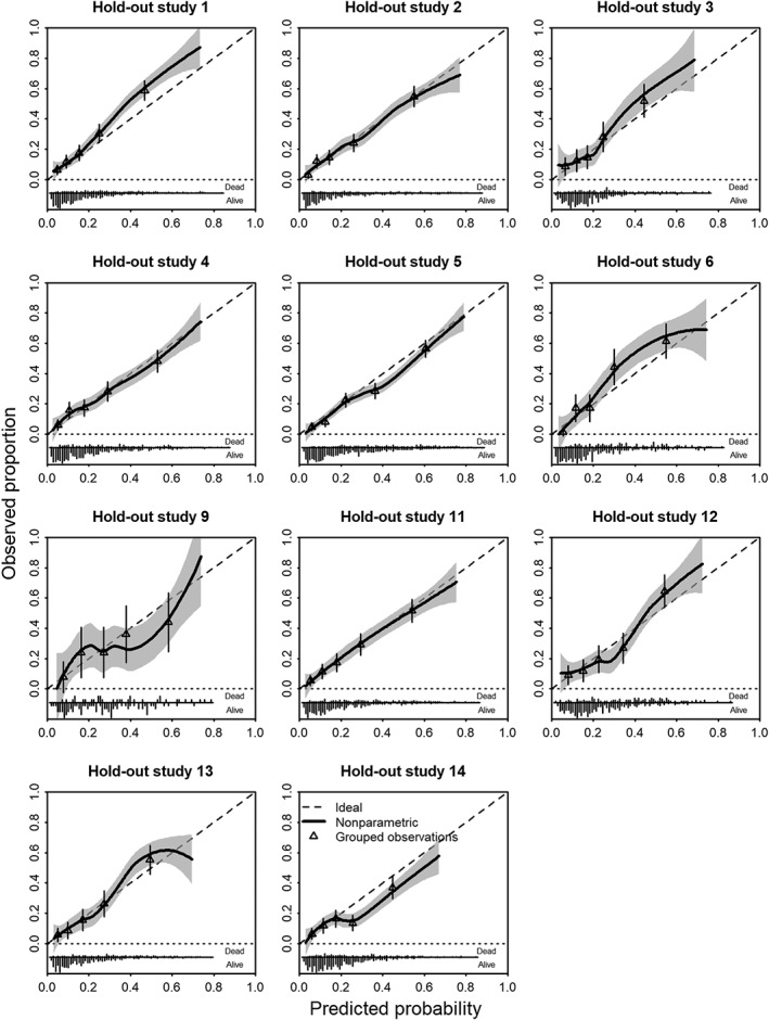
Calibration plots of model developed in RCTs in a leave‐one‐study‐out cross‐validation

6.2. Heterogeneity in discrimination of predictions

Discrimination of prediction models is commonly assessed by a concordance statistic (c).6 We assessed the discriminative ability of the proposed prediction model in a similar fashion as the calibration, again using “internal‐external” cross‐validation stratified for observational studies and RCTs. The common estimate was c = 0.86, with a 95% confidence interval from 0.84 to 0.87 for observational studies (Figure 7). The approximate 95% prediction interval was identical to the 95% confidence interval as there was no evidence of heterogeneity in observed c‐statistics across the observational studies. For the RCTs, the pooled estimate was c = 0.76 with a 95% confidence interval from 0.74 to 0.78 and a 95% prediction interval from 0.71 to 0.81. This reflects the heterogeneity across studies in predictor effects, but also in case‐mix, since the c‐statistic depends on the combination of predictor effects and case‐mix.37, 38

Figure 7.

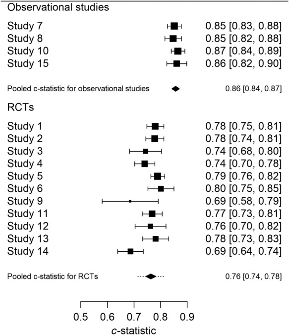
c‐statistics leave‐one‐study‐out cross‐validation

The 95% prediction intervals may be interpreted as plausible ranges for the c‐statistics of the proposed model in a new observational setting or in a new RCT. The observed c‐statistic for the observational studies was higher, in line with the larger case‐mix heterogeneity in patients as compared to the RCTs (Table 2).

7. CASE STUDY SUMMARIZED

In our case study, we found substantial heterogeneity in baseline risk and predictor effects of a fully stratified model. Using the approximate closed‐test procedure, we found that the rank = 1 model was the most appropriate model, rather than the initially proposed global model with common effects for the regression coefficients.12 The observed heterogeneity in slope of the rank = 1 model could largely be explained by whether a study was a trial or an observational study. Substantial heterogeneity in the baseline risk remained present after adjustment for study type. This was especially pronounced for the observational studies. These results argue for two separate models, ie, one for trials and one for observational studies, each with further local adjustment for the baseline risk (the model intercept).

The heterogeneity in baseline risk was clear in the internal‐external validation approach for calibration for the observational studies, while the calibration was less heterogeneous across trials. The c‐statistic was higher for observational studies, reflecting the larger case‐mix heterogeneity and stronger predictor effects in these studies as compared to trials. The steps taking in this assessment of the case study are summarized in Figure 8.

Figure 8.

Schematic representation of the research questions to be answered for the development and validation of a prediction model in an individual patient data meta‐analysis [Colour figure can be viewed at wileyonlinelibrary.com]

In conclusion, these results suggest that two separate models are needed for different purposes. If the goal is to use the model for use in general care, the model based on the observational studies may be the better choice. In contrast, the model based on the RCTs may be the better choice if the model is used for risk stratification of patients participating in a randomized trial.

8. DISCUSSION

In this overview, we considered the assessment of various aspects of heterogeneity in the context of a MA for prediction models. The assessment of heterogeneity in baseline risk, and each of the predictor effects per se, is rather similar to standard MA, except for the multivariate nature of MA of multivariable regression coefficients from multiple studies. More challenging is the assessment of heterogeneity in combinations of baseline risk and predictor effects (Section 5), and heterogeneity in absolute risk and model performance (Section 6).

8.1. Heterogeneity in IPD MA

We first discussed the assessment of between‐study heterogeneity in design, predictors, and endpoints (Section 3). Specifically, a membership model may be valuable to assess between‐study heterogeneity in case‐mix distributions, and to identify outlier studies.16 In the case study, there was however only a weak relation between‐study characteristics and deviating baseline risk or deviating predictor effects. Some trials had a lower mortality, which may be related to the selection of somewhat more favorable patients, while this selection was not fully captured in the observed covariates. In other cases, the baseline risk may be related even more directly to study characteristics. As an example from a very different clinical field, we found a substantially higher probability of indolent prostate cancers among screened patients compared to clinically presenting patients.39

Next, methods to deal with missing values are essential in the context of multivariable prediction modeling, since a few missing values over different predictors may cause a substantial loss in efficiency in a complete case analysis (Section 4). Moreover, some variables may be systematically missing in some of the studies. Several methods to deal with sporadically and systematically missing values in an IPD‐MA have been proposed that aim to maximize congeniality between the imputation and the analysis model. Although it has been demonstrated that multilevel imputation models with a random slope are uncongenial, the resulting bias is often negligible. In the case study of TBI patients, three sets with increasingly complex prediction models were originally proposed, with exclusion of studies for more complex prediction models if predictors were systematically missing.12 The problem of systematically missing variables was also noted in most of 15 IPD meta‐analyses reviewed recently.11 If imputation is attempted, allowing for between‐study heterogeneity is important, arguing for a more refined procedure than applied in our case study.18, 19, 20, 21

Heterogeneity in predictor effects is straightforward to visualize with forest plots and other standard meta‐analytical approaches (Section 5). We may debate whether the choice of predictors for the prediction models should be influenced by the amount of heterogeneity. If the effect is relatively strong but heterogeneous, the first check should be whether there are explanations for the heterogeneity, such as issues in the operationalization of the predictor. If not, we propose that such a strong predictor be kept in the model. The heterogeneity will be reflected in extra uncertainty in prediction intervals (Section 6). Additionally, apparent heterogeneity may be explained by missed nonlinear associations between predictors and outcome, or not including relevant interactions in the global model.

Heterogeneity in absolute risk is what matters ultimately for prediction models (Section 6). This heterogeneity may be driven by heterogeneity in baseline risk in many cases. It is the focus of quality of care research, where specialized centers may claim better results than others, eg, a lower surgical mortality, also related to the volume of care delivered.40 For comparison of predicted absolute risks, the 1‐to‐1 comparisons capture all information (Figure 3). In a variant of this plot, we might standardize the baseline risk, such that the focus shifts to heterogeneity in predictor effects. Figure 3 shows the predicted risks for all available predictor combinations, which is related to attempting to assess the strongest type of calibration, ie, the comparison of observed to predicted risk for individual covariate patterns.34 Validation by predicted risk (rather than specific covariate patterns) is standard for prediction models, and, as illustrated, is readily possible in the context of MA with an internal‐external cross‐validation procedure.16, 35, 36, 41 Both calibration and discrimination can hence be assessed across studies (Section 6). It should also be noted that for internal‐external validation results relatively large studies are required to obtain reliable estimates of study‐specific model performance. Recent studies suggest at least 100 events and 100 nonevents for binary outcomes.42

If there is substantial heterogeneity in baseline risk, the MOR can be a helpful measure to quantify the magnitude of this heterogeneity.43 The MOR is defined as the median value of the odds ratio between the study at the lowest risk and the study with the highest risk when picking two studies at random, or in other words, the increase in risk (in median) of when a patient is included in a study with higher risk of the outcome compared to a study with a lower risk of the outcome.

We recognize that our review and proposals have some limitations. Although the test procedure proposed in the manuscript allows for a formal approach to test whether a fully stratified model is needed, similar procedures to choose between fixed and random effects meta‐analyses have been criticized previously. Therefore, it is advised to not only apply the test procedure but also assess the heterogeneity between studies and consider the practical implications of the between‐study heterogeneity.

We focused on prediction of a binary endpoint. Extensions to survival models require further study (Appendix A).44 More case studies are required to evaluate the practical usefulness of different options to both methodological and clinical researchers. We considered the combination of multiple predictors, while much current research aims to quantify the value of new predictors, such as new markers to predict cardiovascular disease, beyond what is possible with traditional predictors.45 The incremental value of a marker may then be studied per study, with MA approaches applied to performance measures such as the increment in discriminative ability (c statistic, possibly with some transformation).9, 46 Moreover, we considered an ideal modeling situation, where we have access to IPD and have the most relevant predictors available in each study. We expand on situations with aggregated data in Appendix B.

8.2. Heterogeneity and global model performance

If a global model is considered reasonable to propose, we are interested in its performance across different settings and populations.41 It is helpful to distinguish reproducibility and transportability.47 A prediction model is reproducible when it performs sufficiently accurate across new patients from the same underlying population. This property can be directly assessed in a single development data set by applying internal validation techniques such as bootstrapping, with random resampling.6, 48 Model transportability, however, requires the model to perform well across samples from “different but related populations.”47 Transportability can be assessed by performing external validation studies, or by adopting nonrandom resampling methods such as internal‐external cross‐validation.36 When the model is reproducible and shows good transportability across several complementary settings, it can be concluded that its generalizability is adequate.49 This claim is stronger if the included studies are more different from the development study. Therefore, the larger the differences between studies, the stronger the test of generalizability. If development and validation samples are quite similar, reproducibility rather than transportability is assessed.16, 47

8.3. Heterogeneity and local performance

Once a global model from an IPD‐MA is developed and validated across multiple studies, we may consider its practical application in a specific local setting.17 If heterogeneity in predictions between settings is substantial, setting specific covariates may be included to explain part of the observed heterogeneity, as was illustrated in our case study. If substantial heterogeneity remains, a global prediction model is suboptimal in some settings. For settings that were included in the IPD MA, either study specific estimates of coefficients may be used, or a suboptimal performance may be acceptable. If the model is however applied in a new setting, not included in the MA, several other options may be considered.

1. Use the global model with the common estimates of baseline risk and common estimates for the predictor effects;

2. Pick baseline risk and/or coefficients from a setting considered most similar to the new setting, based on setting and context specific characteristics;

3. Use the global model as prior information and update the model for the new setting.

Option 3 requires IPD from the local setting. If heterogeneity appears to be substantial, there is an urgent need to gather such local data to update the model. Furthermore, the usefulness of the global model as prior information will be limited as the information in newly collected data will outweigh the information in the global model. Updating methods may start with simple adjustment of the baseline risk to guarantee calibration‐in‐the‐large in the local setting. More extensive updating approaches can be considered, guided by the available sample size.28, 50

9. CONCLUSIONS

Meta‐analytical techniques have a key role in the development of a global prediction model across multiple studies. As illustrated, IPD from multiple studies give excellent opportunities to investigate, quantify, and report any heterogeneity in the baseline risks, predictor effects, predictions, and performance of a prediction model. We expect that such IPD meta‐analyses will increasingly be performed and advocate the presented approaches to assessing heterogeneity for model selection and presentation of uncertainty in the chosen model.

APPENDIX A.

EXTENSION TO SURVIVAL DATA

If we have individual survival data and assume proportional hazards for predictor effects, we can estimate the regression parameters β (from the partial likelihood) and the baseline hazard h₀(t) (by the Breslow estimator) in each study separately. This will give an estimate of cumulative survival probability S(t₀| x) at any time t₀ of interest. It also possible to obtain the covariance matrix of $\left(\text{ln}\left({\widehat{\mathit{H}}}_0\left({\mathit{t}}_0\right)\right),\widehat{\mathrm{\beta }}\right)$. The implication is that a prognostic MA for fixed t₀ can be carried out along the lines as described in the main paper. The structure is identical, only the link function is different. Note that censoring is implicitly handled by standard Cox regression analysis.

This analysis can be extended to a set of fixed time points (t₁, t₂, …, t_l). In analogy with the aforementioned, we use the notation (α₁, …, α_l) for (ln(H₀(t₁)),…, ln(H₀(t_l)). A model for (α₁, …, α_l) can be based on models for time‐varying frailties51 and generalized further.52 Such a meta‐model provides insight in a prognostic survival model and the between‐study heterogeneity under the assumption of proportional hazards within each study. It can also be used to obtain conditional survival probabilities P(T > t + w ∣ T ≥ t, x) under proportional hazards.

Conditional prognostic models that relax the proportional hazards assumption can be obtained by applying the landmark approach.53 Using a fixed prediction window, the models are similar to the model with fixed t₀ described above and can be analyzed in the same way. Moving the landmark point of prediction gives insights in the development of heterogeneity over time.

APPENDIX B.

META‐ANALYSIS WITH AGGREGATED DATA

B.1. Individual patient data from one study, same predictors

Rather than having access to IPD from all studies considered for a MA, we only may have access to IPD from a single study.54, 55 We first consider the hypothetical situation that several studies have reported the same prediction model. In that case, the key missing piece of information is the within‐study correlations S _j (Section 5.1).

The simplest approach to develop a global model is to simply derive common effect estimates for each predictor using separate random effect MA methods, ignoring dependencies between regression coefficients within studies. A more refined method is to fit a generalized random effects model that accounts for within‐study and between‐study covariance of the regression coefficients. A practical difficulty is that the variance‐covariance matrix is only available for the IPD, and usually not reported for the published models. Assuming homogeneous correlations between predictor effects across studies, we may collapse the missing covariance matrices to the observed covariance matrix ${\widehat{\mathit{S}}}_{\text{IPD}}$. Simulation studies have shown that multivariate MA models are fairly robust to errors made in approximating within‐study covariances when only summary effect estimates are of interest. In a third approach, we may apply a Bayesian framework where a summary of the previously published regression coefficients serves as prior for the regression coefficients in the IPD.

In an empirical study, all three aggregation approaches performed similarly, and yielded better predictions than models that were based solely on one study with IPD.56 This was specifically the case if the IPD set was relatively small. Assessing the degree of heterogeneity between IPD and literature findings is crucial for any of these approaches to work, ie, the more homogeneity of predictor effects, the better the MA of previous studies allows for the development of a global model that provides better predictions for the setting where the single IPD data set originates from.

B.2. Individual patient data from one study, models with different predictors

The situation that multiple studies considered the same prediction model may be rare. A more common situation is that multiple studies provide models with different but overlapping sets of predictors. We may consider various approaches for aggregating previously published prediction models, while at least one IPD data set is available.

A first step is to assess the validity of previously developed models for the setting where we have IPD available. Only the most promising models are then further considered for the development of a global model.

An attractive approach is a variant of ensemble learning. We then use stacked regressions to treat the predictions of each published model as a predictor variable of the meta‐model and subsequently create a linear combination of model predictions.57 Models with a negative contribution on the combined prediction are omitted from the meta‐model. This approach works if the models are not strongly collinear; if they are collinear, dropping the correlated but poorer performing model is advisable.57

Finally, MA approaches may be used to develop a global model if multiple studies have reported only on the univariable relations of predictors to an endpoint, rather than multivariable relations. Considering prior information from published studies is particularly relevant when the IPD sample is relatively small and predictor effects are homogeneous. This was the motivation for such an approach in a case study of aortic aneurysm patients.58, 59 We may first meta‐analyze the estimates of the univariable regression coefficients, with standard assessment of heterogeneity in a random effect model. Second, we may estimate the change from univariable to multivariable coefficient in the IPD. This change may then be used as a simple adaptation factor for the pooled univariable regression coefficients.

B.3. No IPD, models with different predictors

Alternative approaches have been proposed that do not even require the availability of IPD.60 A global model is then developed by using information from published associations between predictors of interest, and from correlations between each pair of the predictors of interest. Here, it is assumed that predictor values from the overall population follow a multivariate normal distribution, ignoring any between‐study heterogeneity.

Steyerberg EW, Nieboer D, Debray TPA, van Houwelingen HC. Assessment of heterogeneity in an individual participant data meta‐analysis of prediction models: An overview and illustration. Statistics in Medicine. 2019;38:4290–4309. 10.1002/sim.8296

REFERENCES

- 1. Steyerberg EW, Moons KG, van der Windt DA, et al. Prognosis Research Strategy (PROGRESS) 3: prognostic model research. PLOS Med. 2013;10(2):e1001381. [DOI] [PMC free article] [PubMed] [Google Scholar]
- 2. Wessler BS, Paulus J, Lundquist CM, et al. Tufts PACE Clinical Predictive Model Registry: update 1990 through 2015. Diagn Progn Res. 2017;1(1):20. [DOI] [PMC free article] [PubMed] [Google Scholar]
- 3. Mushkudiani NA, Hukkelhoven CW, Hernández AV, et al. A systematic review finds methodological improvements necessary for prognostic models in determining traumatic brain injury outcomes. J Clin Epidemiol. 2008;61(4):331‐343. [DOI] [PubMed] [Google Scholar]
- 4. Bouwmeester W, Zuithoff NPA, Mallett S, et al. Reporting and methods in clinical prediction research: a systematic review. PLOS Med. 2012;9(5):e1001221. [DOI] [PMC free article] [PubMed] [Google Scholar]
- 5. Van Houwelingen JC, Le Cessie S. Predictive value of statistical models. Statist Med. 1990;9(11):1303‐1325. [DOI] [PubMed] [Google Scholar]
- 6. Harrell FE. Regression Modeling Strategies: With Applications to Linear Models, Logistic Regression, and Survival Analysis. New York, NY: Springer‐Verlag; 2001. [Google Scholar]
- 7. Steyerberg EW. Clinical Prediction Models: A Practical Approach to Development, Validation, and Updating. New York, NY: Springer Science+Business Media; 2009. [Google Scholar]
- 8. Debray TP, Moons KG, Abo‐Zaid GM, Koffijberg H, Riley RD. Individual participant data meta‐analysis for a binary outcome: one‐stage or two‐stage. PLOS ONE. 2013;8(4):e60650. [DOI] [PMC free article] [PubMed] [Google Scholar]
- 9. Debray TP, Moons KG, Ahmed I, Koffijberg H, Riley RD. A framework for developing, implementing, and evaluating clinical prediction models in an individual participant data meta‐analysis. Statist Med. 2013;32(18):3158‐3180. [DOI] [PubMed] [Google Scholar]
- 10. Debray TP, Riley RD, Rovers MM, Reitsma JB, Moons KG. Individual participant data (IPD) meta‐analyses of diagnostic and prognostic modeling studies: guidance on their use. PLOS Med. 2015;12(10):e1001886. [DOI] [PMC free article] [PubMed] [Google Scholar]
- 11. Ahmed I, Debray TP, Moons KG, Riley RD. Developing and validating risk prediction models in an individual participant data meta‐analysis. BMC Med Res Methodol. 2014;14:3. [DOI] [PMC free article] [PubMed] [Google Scholar]
- 12. Steyerberg EW, Mushkudiani N, Perel P, et al. Predicting outcome after traumatic brain injury: development and international validation of prognostic scores based on admission characteristics. PLOS Med. 2008;5(8):e165. [DOI] [PMC free article] [PubMed] [Google Scholar]
- 13. Royston P, Parmar MK. Flexible parametric proportional‐hazards and proportional‐odds models for censored survival data, with application to prognostic modelling and estimation of treatment effects. Statist Med. 2002;21(15):2175‐2197. [DOI] [PubMed] [Google Scholar]
- 14. Higgins JPT, Green S. Cochrane Handbook for Systematic Reviews of Interventions. Chichester, UK: The Cochrane Collaboration; 2008. [Google Scholar]
- 15. Murray GD, Butcher I, McHugh GS, et al. Multivariable prognostic analysis in traumatic brain injury: results from the IMPACT study. J Neurotrauma. 2007;24(2):329‐337. [DOI] [PubMed] [Google Scholar]
- 16. Debray TP, Vergouwe Y, Koffijberg H, Nieboer D, Steyerberg EW, Moons KG. A new framework to enhance the interpretation of external validation studies of clinical prediction models. J Clin Epidemiol. 2015;68(3):279‐289. [DOI] [PubMed] [Google Scholar]
- 17. Wynants L, Vergouwe Y, Van Huffel S, Timmerman D, Van Calster B. Does ignoring clustering in multicenter data influence the performance of prediction models? A simulation study. Stat Methods Med Res. 2016;27(6):1723‐1736. [DOI] [PubMed] [Google Scholar]
- 18. Jolani S, Debray TP, Koffijberg H, van Buuren S, Moons KG. Imputation of systematically missing predictors in an individual participant data meta‐analysis: a generalized approach using MICE. Statist Med. 2015;34(11):1841‐1863. [DOI] [PubMed] [Google Scholar]
- 19. Jolani S. Hierarchical imputation of systematically and sporadically missing data: an approximate Bayesian approach using chained equations. Biometrical Journal. 2018;60(2):333‐351. [DOI] [PubMed] [Google Scholar]
- 20. Resche‐Rigon M, White IR, Bartlett JW, Peters SAE, Thompson SG. Multiple imputation for handling systematically missing confounders in meta‐analysis of individual participant data. Statist Med. 2013;32(28):4890‐4905. [DOI] [PubMed] [Google Scholar]
- 21. Resche‐Rigon M, White IR. Multiple imputation by chained equations for systematically and sporadically missing multilevel data. Stat Methods Med Res. 2018;27(6):1634‐1649. [DOI] [PMC free article] [PubMed] [Google Scholar]
- 22. Audigier V, White IR, Jolani S, et al. Multiple imputation for multilevel data with continuous and binary variables. Statistical Science. 2018;33(2):160‐183. [Google Scholar]
- 23. Kunkel D, Kaizar EE. A comparison of existing methods for multiple imputation in individual participant data meta‐analysis. Statist Med. 2017;36(22):3507‐3532. [DOI] [PMC free article] [PubMed] [Google Scholar]
- 24. Royston P, Sauerbrei W. Multivariable Model‐Building: A Pragmatic Approach to Regression Analysis Based on Fractional Polynomials for Modelling Continuous Variables. Chichester, UK: John Wiley and Sons; 2008. [Google Scholar]
- 25. Burke DL, Ensor J, Riley RD. Meta‐analysis using individual participant data: one‐stage and two‐stage approaches, and why they may differ. Statist Med. 2017;36(5):855‐875. [DOI] [PMC free article] [PubMed] [Google Scholar]
- 26. Austin PC, Merlo J. Intermediate and advanced topics in multilevel logistic regression analysis. Statist Med. 2017;36(20):3257‐3277. [DOI] [PMC free article] [PubMed] [Google Scholar]
- 27. Perperoglou A, le Cessie S, van Houwelingen HC. Reduced‐rank hazard regression for modelling non‐proportional hazards. Statist Med. 2006;25(16):2831‐2845. [DOI] [PubMed] [Google Scholar]
- 28. Vergouwe Y, Nieboer D, Oostenbrink R, et al. A closed testing procedure to select an appropriate method for updating prediction models. Statist Med. 2017;36(28):4529‐4539. [DOI] [PubMed] [Google Scholar]
- 29. Ambler G, Royston P. Fractional polynomial model selection procedures: investigation of type i error rate. J Stat Comput Simul. 2001;69(1):89‐108. [Google Scholar]
- 30. Stram DO, Lee JW. Variance components testing in the longitudinal mixed effects model. Biometrics. 1994;50(4):1171‐1177. [PubMed] [Google Scholar]
- 31. Cox DR. Two further applications of a model for binary regression. Biometrika. 1958;45:562‐565. [Google Scholar]
- 32. Miller ME, Hui SL, Tierney WM. Validation techniques for logistic regression models. Statist Med. 1991;10(8):1213‐1226. [DOI] [PubMed] [Google Scholar]
- 33. Austin PC, Steyerberg EW. Graphical assessment of internal and external calibration of logistic regression models by using loess smoothers. Statist Med. 2014;33(3):517‐535. [DOI] [PMC free article] [PubMed] [Google Scholar]
- 34. Van Calster B, Nieboer D, Vergouwe Y, De Cock B, Pencina MJ, Steyerberg EW. A calibration hierarchy for risk models was defined: from utopia to empirical data. J Clin Epidemiol. 2016;74:167‐176. [DOI] [PubMed] [Google Scholar]
- 35. Royston P, Parmar MK, Sylvester R. Construction and validation of a prognostic model across several studies, with an application in superficial bladder cancer. Statist Med. 2004;23(6):907‐926. [DOI] [PubMed] [Google Scholar]
- 36. Steyerberg EW, Harrell FE Jr. Prediction models need appropriate internal, internal‐external, and external validation. J Clin Epidemiol. 2016;69:245‐247. [DOI] [PMC free article] [PubMed] [Google Scholar]
- 37. Vergouwe Y, Moons KG, Steyerberg EW. External validity of risk models: use of benchmark values to disentangle a case‐mix effect from incorrect coefficients. Am J Epidemiol. 2010;172(8):971‐980. [DOI] [PMC free article] [PubMed] [Google Scholar]
- 38. Nieboer D, van der Ploeg T, Steyerberg EW. Assessing discriminative performance at external validation of clinical prediction models. PLOS One. 2016;11(2):e0148820. [DOI] [PMC free article] [PubMed] [Google Scholar]
- 39. Steyerberg EW, Roobol MJ, Kattan MW, van der Kwast TH, de Koning HJ, Schröder FH. Prediction of indolent prostate cancer: validation and updating of a prognostic nomogram. J Urol. 2007;177(1):107‐112. [DOI] [PubMed] [Google Scholar]
- 40. Finks JF, Osborne NH, Birkmeyer JD. Trends in hospital volume and operative mortality for high‐risk surgery. N Engl J Med. 2011;364(22):2128‐2137. [DOI] [PMC free article] [PubMed] [Google Scholar]
- 41. Austin PC, van Klaveren D, Vergouwe Y, Nieboer D, Lee DS, Steyerberg EW. Geographic and temporal validity of prediction models: different approaches were useful to examine model performance. J Clin Epidemiol. 2016;79:76‐85. [DOI] [PMC free article] [PubMed] [Google Scholar]
- 42. Vergouwe Y, Steyerberg EW, Eijkemans MJC, Habbema JDF. Substantial effective sample sizes were required for external validation studies of predictive logistic regression models. J Clin Epidemiol. 2005;58(5):475‐483. [DOI] [PubMed] [Google Scholar]
- 43. Merlo J, Chaix B, Ohlsson H, et al. A brief conceptual tutorial of multilevel analysis in social epidemiology: using measures of clustering in multilevel logistic regression to investigate contextual phenomena. J Epidemiol Community Health. 2006;60(4):290‐297. [DOI] [PMC free article] [PubMed] [Google Scholar]
- 44. Cai T, Gerds TA, Zheng Y, Chen J. Robust prediction of t‐year survival with data from multiple studies. Biometrics. 2011;67(2):436‐444. [DOI] [PMC free article] [PubMed] [Google Scholar]
- 45. Kaptoge S, Di Angelantonio E, Pennells L, et al. C‐reactive protein, fibrinogen, and cardiovascular disease prediction. N Engl J Med. 2012;367(14):1310‐1320. [DOI] [PMC free article] [PubMed] [Google Scholar]
- 46. Snell KIE, Ensor J, Debray TPA, Moons KGM, Riley RD. Meta‐analysis of prediction model performance across multiple studies: which scale helps ensure between‐study normality for the C‐statistic and calibration measures? Stat Methods Med Res. 2018;27(11):3505‐3522. 10.1177/0962280217705678 [DOI] [PMC free article] [PubMed] [Google Scholar]
- 47. Justice AC, Covinsky KE, Berlin JA. Assessing the generalizability of prognostic information. Ann Intern Med. 1999;130(6):515‐524. [DOI] [PubMed] [Google Scholar]
- 48. Steyerberg EW, Harrell FE Jr, Borsboom GJ, Eijkemans MJ, Vergouwe Y, Habbema JD. Internal validation of predictive models: efficiency of some procedures for logistic regression analysis. J Clin Epidemiol. 2001;54(8):774‐781. [DOI] [PubMed] [Google Scholar]
- 49. Reilly BM, Evans AT. Translating clinical research into clinical practice: impact of using prediction rules to make decisions. Ann Intern Med. 2006;144(3):201‐209. [DOI] [PubMed] [Google Scholar]
- 50. Steyerberg EW, Borsboom GJ, van Houwelingen HC, Eijkemans MJ, Habbema JD. Validation and updating of predictive logistic regression models: a study on sample size and shrinkage. Statist Med. 2004;23(16):2567‐2586. [DOI] [PubMed] [Google Scholar]
- 51. Fiocco M, Putter H, van Houwelingen JC. Meta‐analysis of pairs of survival curves under heterogeneity: a Poisson correlated gamma‐frailty approach. Statist Med. 2009;28:3782‐3797. [DOI] [PubMed] [Google Scholar]
- 52. Putter H, van Houwelingen HC. Dynamic frailty models based on compound birth‐death processes. Biostatistics. 2015;16:550‐564. [DOI] [PubMed] [Google Scholar]
- 53. van Houwelingen HC, Putter H. Dynamic predicting by landmarking as an alternative for multi‐state modeling: an application to acute lymphoid leukemia data. Lifetime Data Anal. 2008;14:447‐463. [DOI] [PMC free article] [PubMed] [Google Scholar]
- 54. Su TL, Jaki T, Hickey GL, Buchan I, Sperrin M. A review of statistical updating methods for clinical prediction models. Stat Methods Med Res. 2016;27:185‐197. [DOI] [PubMed] [Google Scholar]
- 55. Martin GP, Mamas MA, Peek N, Buchan I, Sperrin M. Clinical prediction in defined populations: a simulation study investigating when and how to aggregate existing models. BMC Med Res Methodol. 2017;17:1. [DOI] [PMC free article] [PubMed] [Google Scholar]
- 56. Debray TP, Koffijberg H, Vergouwe Y, Moons KG, Steyerberg EW. Aggregating published prediction models with individual participant data: a comparison of different approaches. Statist Med. 2012;31:2697‐2712. [DOI] [PubMed] [Google Scholar]
- 57. Debray TP, Koffijberg H, Nieboer D, Vergouwe Y, Steyerberg EW, Moons KG. Meta‐analysis and aggregation of multiple published prediction models. Statist Med. 2014;33:2341‐2362. [DOI] [PubMed] [Google Scholar]
- 58. Steyerberg EW, Eijkemans MJ, Van Houwelingen JC, Lee KL, Habbema JD. Prognostic models based on literature and individual patient data in logistic regression analysis. Statist Med. 2000;19:141‐160. [DOI] [PubMed] [Google Scholar]
- 59. Debray TP, Koffijberg H, Lu D, Vergouwe Y, Steyerberg EW, Moons KG. Incorporating published univariable associations in diagnostic and prognostic modeling. BMC Med Res Methodol. 2012;12:121. [DOI] [PMC free article] [PubMed] [Google Scholar]
- 60. Sheng E, Zhou XH, Chen H, Hu G, Duncan A. A new synthesis analysis method for building logistic regression prediction models. Statist Med. 2014;33:2567‐2576. [DOI] [PubMed] [Google Scholar]