

Abstract
Whether hippocampal map realignment is coupled more strongly to position or time was studied in rats trained to shuttle on a linear track. The rats were required to run from a start box and to pause at a goal location at a fixed location relative to stable distal cues (room-aligned coordinate frame). The origin of each lap was varied by shifting the start box and track as a unit (box-aligned coordinate frame) along the direction of travel. As observed by Gothard et al. (1996a), on each lap the hippocampal activity realigned from a representation that was box-aligned to one that was room-aligned. We studied the dynamics of this transition using a measure of how well the moment-by-moment ensemble activity matched the expected activity given the location of the animal in each coordinate frame. The coherency ratio, defined as the ratio of the matches for the two coordinate systems, provides a quantitative measure of the ensemble activity alignment and was used to compare four possible descriptions of the realignment process. The elapsed time since leaving the box provided a better predictor of the occurrence of the transition than any of the three spatial parameters investigated, suggesting that the shift between coordinate systems is at least partially governed by a stochastic, time-dependent process.
Keywords: place cell, hippocampus, tetrode, spatial navigation, attractor map, coherency ratio
Hippocampal pyramidal cells (“place cells”) display remarkable correlations with the position of an animal within an environment (the “place field” of the cell;O'Keefe and Dostrovsky, 1971) (for review, seeRedish, 1999). Both internal (e.g., vestibular and proprioceptive) and external (e.g., exterosensory) cues contribute to the generation of location-specific activity of hippocampal pyramidal cells (O'Keefe, 1976; Sharp et al., 1995; McNaughton et al., 1996; Touretzky and Redish, 1996; Knierim et al., 1998).
To examine the interaction between these positional signals,Gothard et al. (1996a) trained rats to shuttle back and forth along a linear track with a variable start location. This task defines two dissociable spatial coordinate frames: (1) the room alignment—constant relative to the distal cues within the room, (2) the box alignment—constant relative to the distance the rat has traveled from the box. Gothard et al. found that place fields near the box consisted of spikes more tightly clustered in the box-aligned frame, whereas place fields far from the box consisted of spikes more tightly clustered in the room-aligned frame. One possible explanation of this result is that path integration and external cues interact competitively (Gothard et al., 1996a; Samsonovich and McNaughton, 1997; Redish, 1999). Such a competition implies that the transition will occur when the degree of mismatch between internal and external signals reaches some critical value. Alternatively, the result can be explained by a competition between representations of different cue sets (Fenton and Muller, 1996; O'Keefe and Burgess, 1996). These different theories predict different relationships between hippocampal ensemble activity alignments and various spatial and temporal variables. Because the recordings made by Gothard et al. were pooled across trials, only limited aspects of these relationships could be measured. Novel methods presented in this paper allow detection of alignments on a moment-by-moment basis within a trial, which allows more detailed measurement of these relationships.
Realignment of hippocampal representations within an environment has been observed under a number of different cue-conflict situations (O'Keefe and Conway, 1978; Miller and Best, 1980; Kubie and Ranck, 1983; O'Keefe and Speakman, 1987; Shapiro et al., 1989;Sharp et al., 1995; Gothard et al., 1996b; O'Keefe and Burgess, 1996;Knierim et al., 1998), and the questions of the dynamics of the realignment have been addressed by a number of different hippocampal models (Wan et al., 1994; Touretzky and Redish, 1996; Samsonovich and McNaughton, 1997; Redish and Touretzky, 1997b;Redish, 1999), but progress in experimentally discriminating among various possible mechanisms has been hampered by limitations in analytical methods for quantifying the alignment of the hippocampal ensemble activity within a short temporal window. Given a sufficiently large sample of simultaneously recorded neurons, the approach described below enables the examination of the characteristics of this realignment on a moment-by-moment basis. Using this method, we have addressed the questions of whether the realignment occurs at a constant distance from the box, at a constant location relative to the distal cues, at the midpoint between the box and the salient room-aligned cue at the end of the track, or at a constant time after the onset of mismatch (i.e., after leaving the box).
Some of the results in this paper have been published in abstract form (Redish et al., 1999).
MATERIALS AND METHODS
Subjects
Six male, Fischer-344 rats (three 9–12 months and three 27–32 months) were used in this study. Data were pooled across age groups; age-related differences will be left for future study with more subjects. Animals were motivated by food deprivation (but maintained at 80% of ad libitum feeding weight or higher) as well as by medial forebrain bundle stimulation. Water was available ad libitum throughout the day.
Training chronology
All animals were handled 15 min/d for a week and then were tested in the Morris swim task (Morris, 1981) (seeBarnes et al., 1997, for procedural details used). Both hidden-platform and visible-platform versions were used. All animals described in this study successfully completed the visible-platform version of the task.
The animals were then trained on an elevated rectangular track (93 × 43 cm; 10-cm-wide track). The apparatus also had a cross track bisecting its length. Rats were neither encouraged nor discouraged from using the cross track. Briefly, food was available at two corners of the track; two corners were unbaited. Each time the rat touched a corner, the food at the baited corners was replaced if necessary. Thus, the animal could get food by going to an unbaited corner and then back to a baited corner or by going to the other baited corner. Well trained animals learned to alternate between the two baited corners. Animals received one 30 min session per day until they were eating 30–60 times in the session. This typically took 5–8 d. Distal cues were not controlled during this phase of pretraining.
Animals were then trained to shuttle back and forth on a linear track (182 × 16 cm). Distal cues were available around the walls of the room (∼2 m away, large blocks of white and black curtains, and small white and black posters). The cue configuration was maintained throughout the remainder of pretraining as well as during the linear track task (see below). The rats left a start box at one end of the track, proceeded to a barrier at the other end of the track, and returned to the box. After the animal returned to the box, he received a food reward, the box was closed, and the box and track were moved (as a unit) along the direction of the long axis of the track. Reward was never given at the far end of the track, but if the rat did not reach the end of the track, he did not receive food reward after returning to the box, and the box was not moved. “Reaching the end of the track” was measured as having crossed an invisible line 10 cm from the barrier. For the shuttle task, position was monitored from a ceiling camera (Kohu, San Diego, CA) by a user in another room, watching on a video screen, who identified when the animal had crossed the line and told the animal handler after the animal returned to the box. Animals were taught this task by gradually increasing the distance that had to be traveled to receive food reward until they were running all the way to the end of the track and back. Animals received one 30 min session per day until they were running 20–48 laps. This typically took 11–14 d.
At this point in the protocol, the animals were implanted with stimulation and recording electrodes. During the intervening 2–5 d between pretraining and surgery, animals received ad libitumfood and no training. After surgery, animals were allowed 2–5 d to recover. They were then run for 3–5 d on the rectangular track (using the protocol described above) and 5–7 d of shuttling on the linear track (using the protocol described above). This additional pretraining allowed them to get used to carrying the weight of the implanted hyperdrive, headstage, and cable before learning the task used during recording.
The linear track task was performed on the same apparatus and with the same cues as the pretraining shuttle task described above. Briefly, the rat performed the shuttle task, but if the animal paused for greater than a minimum delay within the goal zone (8-cm-long; centered 35 cm from the barrier), he received medial forebrain bundle (MFB) stimulation reward. The animal could receive a maximum of one reward before reaching the turn-around at the barrier end of the track and one reward on the return journey. Although the box and track were moved along the direction of travel after each trial, the goal zone remained at a constant position within the room throughout the task. For behavioral analysis, the animal's position was tracked at 20 Hz from LED lights on a headstage via a ceiling camera (Kohu) (tracking hardware, San Diego Instruments). Crossing of the invisible line near the barrier (to determine if the animal had proceeded to the end of the track) and time spent in the goal zone were monitored automatically using in-house software written for Discovery (DataWave Technologies, Boulder CO). The linear track task is summarized in Figure1.
Fig. 1.

The apparatus consisted of an elevated, linear track (182 × 16 cm), covered with thin, gray carpet. Each trial began with the animal in the closed box (a). The box was opened, and the animal left the box (b). If the animal paused within the goal zone for longer than the minimum delay (variable by day from 0.1 to 1.5 sec) then he received medial forebrain bundle stimulation (c). Animals could earn only one stimulation before crossing the complete journey threshold 10 cm from the barrier (d). After crossing the threshold, animals turned around, and returned to the box (d–f). The animal could earn another stimulation reward on the inbound journey if he paused in the goal zone for longer than the minimum delay (e). When the animal returned to the box, the box was closed (f), and the animal received a small food reward (g). This marked the end of the trial. The box and track were moved (as a unit) along the long axis of the track before the beginning of the next trial (h). Because the goal zone remained constant in room coordinates (goal location indicated by shaded square), local cues provided no information about the location of the goal zone.
Animals received two 30 min sessions on the linear track task per day, separated by a 20 min rest period in a small box adjacent to the track. The minimum delay began at 0.1 sec (providing stimulation even for animals running at very fast speeds) and was increased daily until reaching a maximum of 1.5 sec. Thus, delay remained constant within a day, but was variable from day to day.
Surgery and recording
After completing pretraining, the animals were implanted with a hyperdrive (a microdrive allowing individual manipulations of 12 tetrodes and two EEG probes; Wilson and McNaughton, 1993; Gothard et al., 1996a; Knierim et al., 2000) over the right dorsal CA1 and CA3 regions of the hippocampus (AP −3.8 mm, lateral +2.0 mm). Each tetrode consisted of four twisted 14 μm enamel-insulated nichrome wires (McNaughton et al., 1983; O'Keefe and Recce, 1993;Wilson and McNaughton, 1993). The tetrode tips were gold-plated, resulting in impedances at 1 kHz of 0.5–1.0 MΩ.
At the time of hyperdrive implantation, animals were also implanted with stimulation electrodes, placed stereotaxically into the medial forebrain bundle at AP +0 mm, lateral ±1.9 mm, and ventral 8.5 mm, at a 20° angle. Stimulation electrodes consisted of two twisted 125 μm Teflon-coated stainless steel wires, with the insulation removed from the final 0.25 mm of the two wires. The wire tips were separated vertically by 1 mm.
National Institutes of Health guidelines were followed for all surgical procedures. Briefly, rats were deeply anesthetized with Nembutal (sodium pentobarbital; Abbott Labs, Irving, TX, 32–40 mg/kg, depending on the rat's age), and placed in a stereotaxic apparatus. Bicillin (Wyeth Laboratories; 0.1 cc, i.m. per hind leg) was given to combat infection, the skull was then cleared of skin and fascia, and eight holes were drilled to accommodate jeweler's screws to anchor the implant. Rectangular holes were drilled around the stimulation electrode entry sites. Stimulation electrodes were placed stereotaxically and then cemented in place with dental acrylic. A circular hole was drilled over the dorsal hippocampus on the right side of the brain, at coordinates of ∼3.8 mm posterior to bregma and 2.0 mm lateral to the midline (depending on blood vessel location), into which the hyperdrive array was positioned and cemented in place with dental acrylic. After surgery, children's Tylenol was used to control postoperative pain.
Neural signals were amplified on a headstage with unity gain and then again with variable gain amplifiers (up to 5K, Assembly Hunter amplifiers, NeuraLynx). Neural signals were filtered between 600 and 6000 Hz. All waveforms crossing a threshold were recorded (Cheetah recording system, NeuraLynx). Because a tetrode consists of four closely spaced wires, spikes from different cells produce differentiable patterns on the four channels (McNaughton et al., 1983; O'Keefe and Recce, 1993; Wilson and McNaughton, 1993). Putative cells (clusters in the feature space defined by the four channels) were separated subjectively using in-house software (XClust, M. Wilson; MClust, A. D. Redish). Cells were classified as pyramidal cells or interneurons based on waveform shape, interspike interval histograms, and average firing rate (Ranck, 1973; O'Keefe and Conway, 1978;Kubie and Ranck, 1983). Only cells with firing characteristics typical of pyramidal cells were included in our analyses (Ranck, 1973; Markus et al., 1995; O'Keefe and Conway, 1978). All cells were required to have no interspike intervals <2 msec to ensure that spike trains had physiologically plausible refractory periods consistent with single units (Ranck, 1973; Markus et al., 1995). Spikes recorded while the animal was not moving (speed <7 cm/sec) were dropped from further analyses. Finally, cells were required to fire at least 100 action potentials on the track to be included in further analyses.
Each day, tetrodes were advanced until cells were observed or until each tetrode had been advanced no more than 20–160 μm (depending on the tetrode's proximity to the hippocampus). The recording quality of cells was assessed while the rat rested on a small platform next to the apparatus.
For neurophysiological analysis, a second tracking system was used that followed the animal's position at 60 Hz from the LEDs on the headstage via the ceiling camera (Kohu) (tracking hardware, Cheetah system, Neuralynx).
Analysis methods
Position
The two-dimensional position (x, y) was projected onto a line stretching along the length of the track (measured from the center of the back of the box to the center of the barrier). This produced a one-dimensional measure of position in the room (v), used for all analyses. Only data from the track were analyzed; data taken while the animal was in the box were dropped from all analyses. The animal's running speed was calculated by first smoothing the position data with a 100 msec Hamming window and then measuring the change in position from one sample to the next.
Journey
A lap was defined as an excursion from the start box. That is, each time an animal left and returned to the box, he had completed one lap, whether or not he had proceeded far enough along the track to complete the trial, and whether or not the box was closed between excursions (Fig. 2). Laps were separated into outbound and inbound journeys by dividing the lap at the maximum point of travel. Thus, all laps consisted of one outbound journey followed by one inbound journey. It is important to note that the outbound journeys did not consist of only outbound motion; animals occasionally turned around to retrace part of a path and then continued in the outbound direction. Inbound journeys were similarly heterogeneous.
Fig. 2.

Definition of the terms trial, lap, and journey. Plot shows a 5 min portion of one animal's position record.Heavy lines crossing the bottom of the trace indicate the front of the start box; heavy line crossing thetop of the trace indicates the complete journey threshold. Each trial consisted of leaving the start box, crossing the complete journey threshold, and returning to the box. The box was moved between trials. Each lap consisted of leaving the box and returning to it, whether or not the animal reached the complete journey threshold. Outbound and inbound journeys divided each lap at the maximal point of travel on that lap. Note that one trial could include multiple laps (but had to include at least one), but each lap included only one outbound and one inbound journey (data from session 6591 LT 25 a).
Spike-density histograms versus place fields
The spatial aspects of hippocampal pyramidal cell activity are commonly quantified as the place field of the cell (O'Keefe and Dostrovsky, 1971): typically the action potentials of each cell are plotted as a function of the animal's position at the time each spike occurred. The resulting histogram is then normalized by the amount of time the animal spent at each location (Muller et al., 1987). Such occupancy-normalized firing rate histograms are not useful, however, for experiments such as this one, in which pyramidal cell activity is analyzed over independently shifted spatial coordinate systems. The normalization leads to a systematic distortion because space is not identically sampled in the two coordinate systems. This is illustrated in Figure3a, which shows the average time spent by the animals at each location on the track as measured in the room-aligned coordinate system. Note that the occupancy was fairly consistent over most of the track, but dropped off linearly in the area encompassed by the variable start location. This occurs because an animal will only be able to occupy the positions near zero when the track is at its longest configurations. At shorter track configurations, the animal will be physically unable to reach the positions near zero. A similar argument explains Figure 3b, in which the average time spent by the animals at each location on the track as measured in the box-aligned coordinate system was fairly consistent over most of the track but dropped off linearly near the barrier.
Fig. 3.
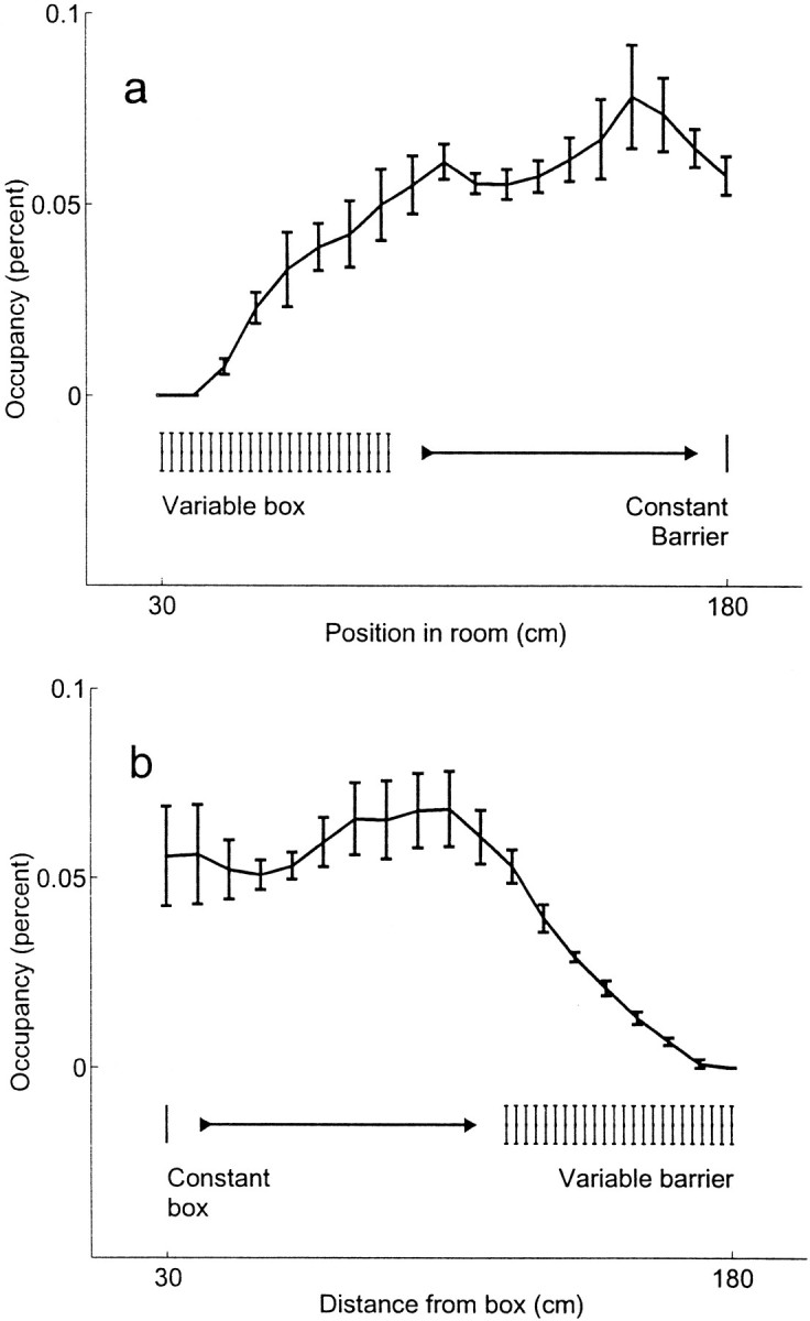
Occupancy in the two coordinate systems. Line indicates the median proportion of time spent at each location over all animals over all sessions (n = 6 animals, bars indicate SE). a, Occupancy as a function of position in the room-aligned coordinate frame. The barrier remains at a constant position, but the box is moved with each trial. The sharp drop in occupancy in the left portion of the figure is caused by the variable starting box location. Note that in the area not affected by the variable starting box location, the occupancy is nearly constant. b, Occupancy as a function of position in the box-aligned coordinate frame. In this coordinate frame, the box remains constant, but the distance from the box to the barrier changes. This variability in available length of the track produces the sharp drop in occupancy in the right portion of the figure. Again, note that in the area not affected by the variable length of the track, the occupancy is nearly constant.
The effect this has on place fields can be seen in the cell shown in Figure 7. This cell fired at the end of the track near the barrier. Observing the data, this cell can be qualitatively described as firing at a consistent location in the room-aligned coordinate frame (see Fig.7b). Because the starting box covers a range of ∼60 cm, the distribution of the animal's locations measured in box-aligned coordinates at which the cell fired a spike is spread out relative to the distribution of locations measured in the room-aligned coordinate frame (Fig. 7a). However, the overall locations sampled by the animal are not also spread out evenly: the farthest reaches of the box-aligned coordinate system can only be sampled at the longest track configuration. Therefore the place field appears distorted in the box-aligned coordinate frame (see Fig. 7e).
Fig. 7.

A typical cell with firing (in this experiment) related to position in the room. a, Box-aligned firing.Line indicates journeys out and back; dotsindicate spikes fired by the cell (only spikes occurring while the animal was on the track are shown). Note the lack of consistent spatial firing. b, Room-aligned firing. Same data as in a, but plotted according to position in room. c, SDH of the cell measured in the box-aligned coordinate system. d, SDH of the cell measured in the room-aligned coordinate system. e, PF of the cell measured in the box-aligned coordinate system. f, PF of the cell measured in the room-aligned coordinate system (data from cell TT6.3 from session 6650 LT 08 a). Compare Figure 6.
Note that the cell shown in Figure 6 does not show this same distortion because the field of the cell lies in the midrange of the track. However, a cell with a box-aligned place field that lay very close to the box would have a distorted place field measured in the room-aligned coordinate frame. In other words, place fields near the barrier are distorted when measured in the box-aligned coordinate frame (as shown in Fig. 7e), place fields near the box are distorted when measured in the room-aligned coordinate frame (data not shown), and place fields in the middle of the track are not distorted in either coordinate frame (see Fig. 6). This distortion is entirely attributable to spatial sampling at the extremes of the track.
Fig. 6.

A typical cell with firing (in this experiment) related to distance from the box. a, Box-aligned firing.Line indicates journeys out and back; dotsindicate spikes fired by the cell (only spikes occurring while the animal was on the track are shown). b, Room-aligned firing. Same data as in a, but plotted according to position in room. Note the lack of consistent spatial firing. c,SDH of the cell measured in the box-aligned coordinate system. d, SDH of the cell measured in the room-aligned coordinate system. e, Place field (PF) of the cell measured in the box-aligned coordinate system. f, PF of the cell measured in the room-aligned coordinate system (data from cell TT4.1 from session 6650 LT 08 a). Compare Figure 7.
The “coherency ratio” measurement used in this paper (see below) assumes that the spatial firing fields of each cell within a fixed coordinate frame can be approximated by a Gaussian. Although place fields on linear tracks do show some skew even in tasks in which space is held constant (Mehta et al., 1997), the distortion from a Gaussian is small enough not to affect the calculations. However, the distortion of place fields shown in Figure 7e is too far deviated from a Gaussian, and it makes the calculation of the coherency ratio unsound if place fields are used.
One alternative is to calculate a spike-density histogram (SDH). This method simply leaves out the occupancy normalization. This is valid because, over the course of many trials, the rats in this study occupied each position for approximately the same amount of time (except, of course, in the range of the tails produced by the variable start location). As shown in Figure 3, the spatial sampling was nearly constant over the part of the journey not covered by the variable box (in the room-centered coordinate frame; Fig. 3a) or the variable barrier (in the box-centered coordinate frame; Fig.3b). This means that although spike density histograms are, in general, sensitive to the animal's behavior, in this study, the behavior was consistent enough to allow their use. As shown in Figure7, c and e, calculating SDHs produces clean spatial fields that are more qualitatively similar to those seen in tasks with a constant spatial coordinate frame. Thus, hereafter the terms “field” and “spatial firing field” shall refer not to a place field, but to a spike-density histogram.
The coherency ratio
The coherency ratio is a means of comparing the quality of a distributed representation of position within two coordinate systems on a moment-by-moment basis. For each coordinate system, the ensemble activity within a brief time window is compared to the expected ensemble activity given the actual position of the rat in that coordinate system. In other words, the coherency for a coordinate system measures how typical the ensemble activity observed within that time window is when compared to ensemble activity in experiments with a constant spatial coordinate frame. The ratio between the coherency measured for each coordinate system gives a quantitative measure of which coordinate system is better represented by the ensemble activity in that time window.
Finding the coherency ratio entails three major steps: (1) finding the activity packet (see below) in each coordinate system—this measures the spatial correlates of the ensemble activity at a moment in time, (2) finding the coherency of the representation in each coordinate system by comparing the actual activity packet with the expected activity packet—this measures how typical the ensemble activity is relative to the expected activity given the position of the animal at a moment in time, and (3) taking the ratio between the coherencies in the two coordinate systems. Because a larger coherency indicates a better fit between the observed and expected ensemble activity, taking the ratio enables a comparison between how typical the observed ensemble activity in each coordinate system is.
Although the coherency ratio is well defined for a two-dimensional environment and can be easily generalized to any input parameters (such as, for example, orientation of a visual stimulus for visual cortex ensemble activity), for simplicity, it is presented for a one-dimensional environment here.
Step 1: the activity packet. The activity packet is a measure of the ensemble activity within a brief time window. The definition of the activity packet presented here is equivalent to the definition used by Samsonovich and McNaughton (1997).
Let SiC(v) be the spike-density-histogram for cell i, i.e., the number of spikes fired, over all trials, by cell i while the animal was at position v in coordinate frame C, normalized by the total number of spikes cell i fired. This is the spatial firing field of cell i. All spike-density histograms were normalized by the total number of spikes fired by each cell in the session.
Let Fi(t) be the firing rate of cell i at time t. This was measured by taking the number of spikes fired by cell i over a brief time window.
Then the activity packet at time t in coordinate frame C, AtC(v), is defined as the mean of the fields, weighted by the firing rate of each cell. Like the fields themselves, it is a function of position v:
| Equation 1 |
See Figure 4 for a diagram of how to calculate the activity packet from a population of spatial firing fields. Figure 5 shows the average activity packet recorded from a previous experiment on a similar track with a stable starting position (Redish et al., 2000).
Fig. 4.

The activity packet is defined as the sum of the spatial fields, each field weighted by the firing rate of the corresponding cell within a short time-window. Spatial-density fields (SDHs) of three model cells are shown. The activity packet is the sum of five times the top field plus 40 times the middle field plus five times the bottom field, divided by 50.
Fig. 5.

Average activity packet from outbound journeys of an animal shuttling back and forth on a 180 cm (8-cm-wide) linear track (Redish, McNaughton, and Barnes, unpublished data); some of the results from this pilot experiment were reported in Redish et al. (2000). For this pilot animal, neither track nor box were moved. For each outbound journey, activity packets were calculated at 1 sec intervals as described in Materials and Methods. Activity packets were all aligned to the current position of the animal. Bars show mean activity packet (error bars show SEM). Solid line shows Gaussian fit of activity packet with ς = 9 cm. The skewness of the activity packet is likely to be a consequence of the backward shift of spatial fields with experience (Mehta et al., 1997) (data from rat #6274; 14 sessions, 593 total laps, average = 42 laps/session, range = 21–67; 273 total cells, average 19.5 cells in ensemble, range = 7–37):
Step 2: the coherency of the activity packet. On a track of 180 cm, in a task with a stable starting position, activity packets are generally well-fit by appropriately centered Gaussians with an SD of 9 cm (A. D. Redish, B. L. McNaughton, and C. A. Barnes, unpublished data from four rats; Fig. 5). This Gaussian G(v) can be taken as a canonical activity packet to which the actual activity packet can be compared. The result of the comparison is the coherency. The coherency, KC(t), of an activity packet at time t is defined as the inner product of the activity packet, AtC(v), and the expected activity packet, Gu(v), centered at the actual position u of the animal in coordinate system C. Because both AtC(v) and Gu(v) are normalized, KC(t) ranges between 0 and 1.
| Equation 2 |
Step 3: the coherency ratio. To quantify which coordinate system is the better indicator of ensemble activity, the coherency ratio is defined as the ratio between the coherency of the activity packets in each coordinate system. Thus, the coherency ratio, R(t), at time t is:
| Equation 3 |
The equations above have been written as if the coherency ratio were measured at an instantaneous time. In the analyses presented below, each journey was divided into 20 equal-duration slices, and the coherency ratio was measured over those time windows (slice duration ranged from 0.5 to 1.0 sec). Firing rate for a cell was measured as total number of spikes fired by that cell during the time window. If no cells fired spikes during the time window, the coherency ratio for that time window was undefined and not considered in further analyses.
Mutual information
Mutual information expresses the amount of information one can deduce about one variable from the value of another variable. In the current study, for example, it was used to answer the following question: how much does knowing the position of the animal in the room-aligned coordinate frame at a given moment in time help one to correctly guess whether or not a realignment occurs at that moment? How much does knowing the position of the animal in the box-aligned coordinate frame help?
Mutual information between two variables a and b, I(a, b), was calculated as the difference between the total entropy of the two variables taken separately, E(a) and E(b), and the entropy of the conjoint distribution of the two variables E(a, b) (Cover and Thomas, 1991). Entropy was measured as the Shannon information required to represent each variable:
| Equation 4 |
where P(x) is the probability of the occurrence of x. Thus, the mutual information was measured as:
| Equation 5 |
Variables were first binned at the resolution at which they were measured. The entropy of these distributions were calculated as described above. Each journey was divided into 20 equal-duration slices (see above). One slice was identified as the transition between representations (outbound journey, first slice with R > 1.0; inbound journey, first slice with R < 1.0). Each slice was then identified as either being the transition point or not. Mutual information between these two distributions was calculated as described above. As noted by Panzeri and Treves (1996), this measure overestimates the actual mutual information. We therefore factored in a correction factor (Panzeri, 1996, their Eq. 2.6). Including the correction factor did not qualitatively change the results.
RESULTS
We recorded 1880 spike trains from six rats over 83 30 min sessions (two sessions per day). Recordings were taken from the CA1 and CA3 regions of the hippocampus. Most of the cells recorded were from the CA1 region, but some tetrodes were located in the CA3 region. Differences between these two regions were not considered in our analyses.
Field centers and field slopes
As noted by Gothard et al. (1996a), on the early parts of the outbound journeys, the firing tended to correlate with the rats' distance from the box. Later, firing tended to correlate with the rats' position in the room. The opposite effect occurred on the return journey. This tendency can be quantified for each cell by measuring the correlation of the components of its field with the starting box location (the slope of the field; Gothard et al., 1996a). Slopes near 1.0 indicate cells that, in this experiment, fired in relation to the rat's distance from the box, whereas slopes near 0.0 indicate cells that, in this experiment, fired in relation to the rat's position in the room. Figure6 shows a cell with a field tightly tied to the starting box location (slope = 0.85), and Figure7 shows one with a field unrelated to the starting box location (slope = 0.19). Figure8a illustrates the high correlation (i.e., large slope) of the position of the field of the first cell with the starting box location. Figure 8b, conversely, illustrates the low correlation (i.e., small slope) of the position of the field of the second cell with the starting box location. Instead, this second cell tended to fire at a consistent position in the room.
Fig. 8.

a, Slope of the field of the cell shown in Figure 6. Each spike fired by the cell is plotted relative to the starting position of the lap and the position of the animal in the room at the time of the spike. Note the consistent firing relative to the variable starting position. b, Slope of the field of the cell shown in Figure 7. Each spike fired by the cell is plotted relative to the starting position of the lap and the position of the animal in the room at the time of the spike. Note the consistent firing relative to position in the room.
Also as noted by Gothard et al. (1996a), fields with a particular slope were not randomly distributed along the track: cells with fields near the box tended to fire in relation to the rat's distance from the box (high slope), whereas cells with fields far from the box tended to fire in relation to the position in the room (low slope). Figure 9 shows, for all cells recorded, the slope of the field of each cell versus the position of the field of the cell in the room. There was a significant relationship between the slope of the field and the position of the field in the room in each of the six animals during both the inbound and outbound journeys (one-factor ANOVA; outbound, P < 10−10, df = 14, 1550, F = 18.37; inbound: P < 10−10, df = 13, 1457, F = 20.12). These results essentially replicate those of Gothard et al. (1996a).
Fig. 9.
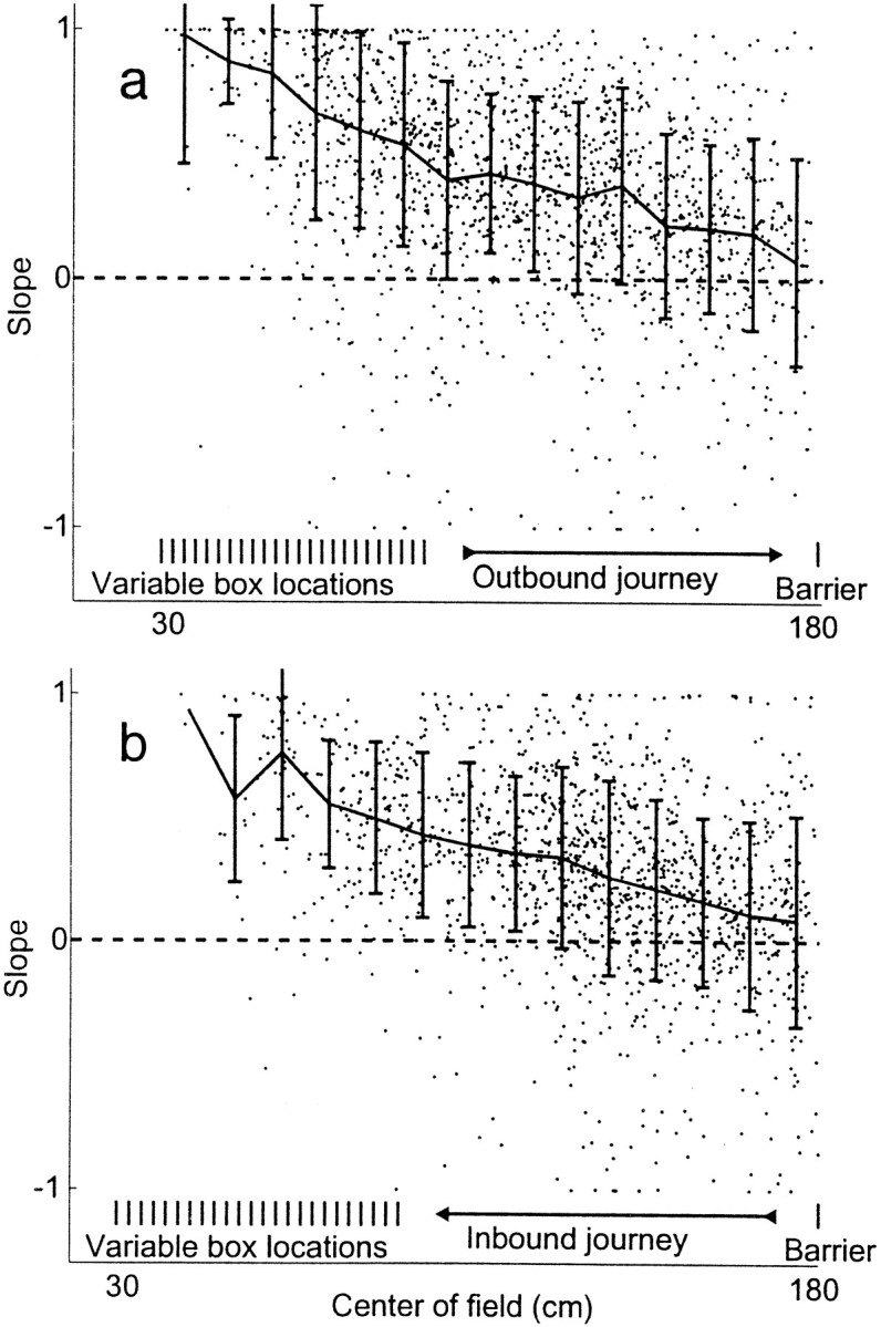
Slopes of all spatial firing fields recorded from all animals as a function of the median position of the spatial firing field. Slope was calculated as correlation of firing with starting position (i.e., the field of the cell shown in Fig. 6 had a slope of 0.85, and the field of the cell shown in Fig. 7 had a slope of 0.19). a, Outbound fields. b, Inbound fields.Heavy lines with error bars indicate SD around the median. This replicates the findings of Gothard et al. (1996a).
The hippocampal ensemble changes alignment across the journey
Because multiple cells (average = 22; range = 8–46) were recorded simultaneously in each session, questions can be asked about the properties of the hippocampal ensemble. To address the question of whether the ensemble progresses from a wholly box-related representation to a wholly room-related representation, expected values for the coherency ratio need to be determined given completely box-aligned or completely room-aligned activity. We first derive quantitative predictions for these two values, then, by measuring the coherency ratio over the first and last 10% of each outbound and each inbound journey, we show that the predictions closely approximate the actual observations.
The coherency ratio: expected values
From the properties of the track, it is possible to calculate expected values for the coherency ratio given a completely box-aligned activity packet and a completely room-aligned packet (see ). These calculations are quantitative predictions derived from the theory that the hippocampal ensemble activity represents position within either one spatial coordinate system or the other.
The derivation starts from three critical assumptions: (1) spatial fields can be approximated by Gaussians of width ςp, (2) activity packets in some coordinate system (hereafter referred to as the ideal coordinate system) can be approximated by Gaussians of width ςg, and (3) the coordinate system being measured is shifted over time (in this experiment, trial by trial) from the ideal coordinate system by a uniform random distribution which has the effect of spreading spatial fields by a factor γ. The derivation thus begins with:
| Equation 6 |
where x0 is the location of the animal in the coordinate system being measured (spanned by x), Gx0(x) is the Gaussian fit to the expected activity packet, Fy(x0) is the firing rate of the cell centered at location y given that the animal is at location x0, and Pyγ(x) is the spatial field of the cell with field center y measured in the space spanned by x, which is shifted from the ideal coordinate system by factor γ. The derivation thus assumes an infinite space (spanned by the variable x ∈ [−∞, +∞]), spanned by a continuous population of fields (with centers y ∈ [−∞, +∞]).
The expected coherency K for an activity packet measured in a coordinate system shifted by γ from the ideal coordinate system is:
| Equation 7 |
where ςp is the typical width of a place field in the ideal coordinate system, and ςgis the width of the expected activity packet in that coordinate system. Thus, the coherency ratio between packets measured in the two coordinate systems (room-aligned shifted by γrrelative to the ideal coordinate system, and box-aligned shifted by γb relative to the ideal coordinate system) is:
| Equation 8 |
The linear track used in this experiment was 182-cm-long; the starting position could vary by as much as 60 cm. Estimates for ςp and ςg were determined from previously recorded pilot data, in which animals shuttled back and forth on a 180 cm linear track with a constant start (Redish, McNaughton, and Barnes, unpublished data). Average spatial field width (ςp) was measured as the average SD of the spike density histograms of all cells firing >100 spikes on the track. Average spatial field width was 20 cm. For a completely box-aligned activity packet, the box-aligned coordinate system is unshifted relative to the ideal coordinate system (by definition), so γb = 1, and because the box moves by up to 60 cm, the room-aligned coordinate system is shifted by a factor γr = 60 cm/20 cm = 3. For a completely room-aligned activity packet, the room-aligned coordinate system is unshifted relative to the ideal coordinate system (by definition), so γr = 1, and by the same argument made in the previous sentence, γb = 3. Average activity packet width (ςg) was measured by measuring the activity packet over a 1000 msec time window every 1000 msec. Average activity packet width was 9 cm. Given these measurements and Equation8, the expected coherency ratio of an ideal room-aligned packet will be 1.6 and that of an ideal box-aligned packet will be 0.6.
Neurophysiology
On the outbound journey, the typical coherency ratios started near 0.6 and ended near 1.6 for all six animals (Fig.10a), whereas on the inbound journey, the coherency ratios started near 1.6 and ended near 0.6 for all six animals (Fig. 10b). Thus, at the beginning of the outbound journey, as the animal left the start box, the hippocampal activity reflected position wholly aligned to the box, but as the animal turned around (ending the outbound and beginning the inbound journey), hippocampal activity reflected position wholly with respect to the room. Then, as the animal returned to the box (completing the inbound journey), the hippocampal activity patterns returned to a representation wholly aligned to the box.
Fig. 10.

Coherency ratio at the start and end of each journey. a, Outbound journey. Black circlesindicate median coherency ratio over the first 10% of the journey (as the animal left the box); gray squares indicate median coherency ratio over the last 10% of the journey (as the animal reached the barrier). Dashed lines indicate predictions from the expected coherency ratio (derived in ). b, Inbound journey. Gray squares indicate median ratio over the first 10% of the journey (as the animal left the barrier); black circles indicate median coherency ratio over the last 10% of the journey (as the animal reached the box). Error bars show SEM.
Transitions between alignments
The result above demonstrated a shift in the ensemble activity from a box-aligned to a room-aligned reference frame across the journey. Because the coherency ratio enables a moment-to-moment analysis of the system, it can be used to determine when the actual transition occurred. This time-of-transition can be used to examine the consistencies in the dynamics of the realignment process.
Consistencies in the dynamics were addressed by dividing each outbound and each inbound journey into 20 equal-duration time slices and measuring the coherency ratio at each time slice. Because (by definition) a coherency ratio R > 1.0 implies a more room-aligned representation, whereas a coherency ratio R < 1.0 implies a more box-aligned representation, the first time slice with a ratio R > 1.0 was identified as the transition (note that, because R is a ratio, R = 1.0 when the two measured coherencies are equal).
Figure 11 shows one outbound journey from one animal. The transition point is identified as the slice occurring ∼7.5 sec after the animal left the box. Although this transition measure is noisy, by looking at a population of many transitions (55–700 per animal), consistencies can be identified.
Fig. 11.

Change in coherency ratio over a single outbound journey from a single animal. The outbound journey was divided into 20 equal-duration time slices (only 14/20 time windows included spikes; others are not shown). The coherency ratio was measured at each time window. Early time windows had coherency ratios near 0.6, late windows had ratios near 1.6. The first time window with a coherency ratio R > 1.0 (i.e., better aligned to room coordinates than to box coordinates) was defined as the transition point (indicated bycircled point). On this journey, the transition point occurred ∼8 sec after the animal left the box (data from lap 2 of session 6591 LT 25 a, 29 cells in ensemble).
From distributions of the transitions, consistencies in four domains were measured: (1) location of animal in the room-aligned coordinate frame, (2) location of the animal in the box-aligned coordinate frame, (3) location of the animal relative to the midpoint between the box and the barrier, and (4) time since the animal began the journey. These four hypotheses derive from published theories that explain aspects of hippocampal spatial activity (McNaughton et al., 1996;Touretzky and Redish, 1996; O'Keefe and Burgess, 1996; Samsonovich and McNaughton, 1997;Redish, 1999): (1) rats might use path integration information for a certain distance from the box, after which they may switch to the information available from the distal visual cues. This hypothesis predicts that transitions should have distributed as a Gaussian centered around a specific point in the box-aligned coordinate frame. (2) Alternatively, the transition might occur when the rats see a specific visual cue or group of cues. This hypothesis predicts that transitions should have distributed as a Gaussian centered around a specific point in the room-aligned coordinate system. (3) A third possibility is that specific landmarks might exert control over their own local space: representations would be sensitive to distance from the box (i.e., box-aligned) when the animal is closer to the box and sensitive to distance from the barrier (i.e., room-aligned) when the animal is closer to the barrier. This third hypothesis predicts that transitions should occur at approximately the half-way point of the journey. (4) The fourth hypothesis is that place cells are part of a dynamic system in a semi-stable state that can cross into another semistable state only after surpassing an energy barrier. This predicts that transitions should at least partially depend on the time elapsed since the mismatch between the sensory and idiothetic cues occurred.
Outbound journeys
Figure 12 shows histograms of transitions from all outbound journeys by a single animal. The distributions of transitions in the three spatial domains did not show reliable consistencies, but the distribution in the temporal domain was well fit by a log-normal distribution. All six animals showed distributions similar to the examples shown in Figure 12.
Fig. 12.

The distribution of transition points over all outbound journeys from a single animal. a, Distribution of transitions as a function of distance from the box. b, Distribution of transitions as a function of position within the room. c, Distribution of transitions as a function of midpoint between box and barrier. d,e, Distribution of transitions as a function of time since the animal began the outbound journey. d, Time plotted linearly. e, Time plotted logarithmically. A Gaussian function has been fit to the distribution of transition times with time plotted on a logarithmic axis (e,heavy line) (data from animal 6591).
Because the scales are different for time and space, it is impossible to compare the histograms in Figure 12 directly. Therefore, we measured the mutual information (Cover and Thomas, 1991) between each of these four domains (time since leaving the box, room-coordinates, box-coordinates, and position relative to the midpoint between box and barrier) and whether the time slice contained a transition point or not. In other words, the mutual information between the temporal domain and the occurrence of a transition expressed how much knowing the answer to the question, “How much time has passed since the animal left the box?” helped one to answer the question, “Did a realignment occur at time t ?” Similarly, the mutual information between the spatial domain of the room and the occurrence of a transition expressed how much knowing the answer to the question, “Where is the animal in the room-aligned coordinate frame?” helped one answer the question, “Did a realignment occur at location x ?” For all six animals, time since leaving the box provided more information than room-aligned, box-aligned, or midpoint-aligned coordinates, indicating that the transitions were more consistent in time than in any spatial domain (two-tailed sign-test; P = 0.032 for all comparisons between time and each factor; Siegel, 1956). See Figure13a.
Fig. 13.

Mutual information between occurrence of the transition and time since the animal began the journey, position of the animal in the room, distance of the animal from the box, and position of the animal relative to the midpoint between the box and the barrier. A higher mutual information indicates that the measure is a better predictor of the occurrence of the transition. These data have been corrected for sample bias using the correction suggested byPanzeri (1996) (see Materials and Methods). Whether the correction factor was included or not did not qualitatively change the results (i.e., time still provided more information). a, Outbound journeys. Note that time provided more information than position in room (6 of 6, p = 0.032, two-tailed sign test), than distance from box (6 of 6, p = 0.032, two-tailed sign test), and than position relative to the midpoint between box and barrier (6 of 6, p = 0.032, two-tailed sign test). b, Inbound journeys. Note that again time provided more information than position in room (6 of 6, p = 0.032, two-tailed sign test), than distance from box (6 of 6, p = 0.032, two-tailed sign test), and than position relative to the midpoint between box and barrier (6 of 6, p = 0.032, two-tailed sign test).
Because the temporal distribution shown in Figure 12e was well approximated by a log-normal distribution, average time to transition was measured as the geometric mean, and the SEM was measured as the geometric SE (Rees, 1987; Limpert, 1999). The geometric mean of the time to transition for the outbound journeys ranged from 5 to 18 sec but remained approximately constant for each animal (SE of the geometric mean ranged from 3 to 18%). Similar results were obtained using the median of the distribution (Table 1).
Table 1.
Mean spatial and temporal coordinates of the hippocampal realignment
| Outbound journey | ||||||
| Animal | 6504 | 6591 | 6608 | 6649 | 6650 | 6682 |
| Geometric mean time to transition (sec) | 17.81 | 6.81 | 6.88 | 7.69 | 5.34 | 9.90 |
| SE | 16% | 3% | 4% | 8% | 6% | 18% |
| Mean room-coordinate of transition (cm) | 124 ± 34 | 121 ± 31 | 109 ± 30 | 126 ± 33 | 118 ± 29 | 117 ± 32 |
| Mean track-coordinate of transition (cm) | 67 ± 34 | 64 ± 32 | 52 ± 32 | 79 ± 30 | 65 ± 34 | 54 ± 36 |
| Mean midpoint-coordinate of transition (cm) | 4 ± 32 | 1 ± 30 | −6 ± 30 | 11 ± 30 | 1 ± 30 | −7 ± 33 |
| Inbound journey | ||||||
| Animal | 6504 | 6591 | 6608 | 6649 | 6650 | 6682 |
| Geometric mean time to transition (sec) | 12.48 | 3.02 | 5.48 | 2.27 | 3.27 | 7.98 |
| SE | 21% | 5% | 5% | 11% | 9% | 23% |
| Mean room-coordinate of transition (cm) | 123 ± 44 | 104 ± 41 | 108 ± 42 | 75 ± 38 | 87 ± 42 | 113 ± 42 |
| Mean track-coordinate of transition (cm) | 64 ± 45 | 48 ± 42 | 51 ± 44 | 14 ± 38 | 31 ± 46 | 60 ± 41 |
| Mean midpoint-coordinate of transition (cm) | 0 ± 44 | −14 ± 41 | −9 ± 42 | −46 ± 37 | −32 ± 43 | 3 ± 41 |
Outbound journeys, time measured from when the animal left the start box. Inbound journeys, time measured from when the animal reached his maximal distance from the box on that lap (i.e., when he turned around). Because time distributed log-normally (see Fig.12d,e), mean time was measured using the geometric mean, and SEM was measured as 1/ times the geometric SD. Although the range between animals varied dramatically, mean times to transition remained relatively constant within animal. Three spatial coordinate systems also included room-aligned coordinates, box-aligned coordinates, and position relative to the midpoint between box and barrier (midpoint coordinates). Because spatial coordinates were not normally distributed, values are expressed as median (± SD). Note that a uniform distribution covering the entire track would have a SD of 44 cm. Note also that because of differences between temporal and spatial units, variances of temporal and spatial distributions are not comparable; comparisons were made with mutual information (see Materials and Methods).
Inbound journeys
On inbound journeys, the hippocampal ensemble activity also tended to realign, but from a room-aligned representation (with a coherency ratio R near 1.6) back to a box-aligned representation (with a coherency ratio R near 0.6) (Fig. 10). To measure the consistencies of the inbound realignment, inbound journeys were divided into 20 equal-duration time slices, and transition points on the inbound journey were measured as the first slice with a coherency ratio R < 1.0. As with the outbound journeys, four consistencies were measured: how consistent the transition was relative to the animal's location in the room-aligned coordinate frame, how consistent the transition was relative to the animal's location in the box-aligned coordinate frame, how consistent the transition was relative to the midpoint between the box and the barrier, and how consistent the transition was relative to time elapsed since the animal began the inbound journey. Note that, for the inbound journeys, elapsed time was not measured from the moment the animal left the box, but from the moment the animal began its return to the box after reaching its maximum point of travel on the lap in question (Fig. 2).
Inbound journeys showed the same properties as the outbound: for all six animals, knowing the time elapsed from the beginning of the inbound journey provided more information about the occurrence of a transition than did knowing the animal's location in any spatial domain, indicating that the transitions were more consistent in time than in any spatial domain (two-tailed sign-test; P = 0.032 for all comparisons between time and each factor; Siegel, 1956) (Fig. 13b).
Like the outbound journeys, the distribution of times elapsed between beginning of inbound journey and the transition again distributed log-normally. Therefore, typical times were again measured using geometric mean and geometric SE (Rees, 1987;Limpert, 1999). The geometric mean of the time to transition for the inbound journeys ranged from 3 to 12 sec but remained approximately constant for each animal (SE of the geometric mean ranged from 5 to 23%). Again, median of the distribution provided similar results (Table 1).
DISCUSSION
The current study examined rats navigating in a task which dissociated two coordinate systems: a coordinate system aligned to the box and track (box-aligned; local cues) and a coordinate system aligned to the barrier and the cues around the room (room-aligned; distal cues). As observed by Gothard et al. (1996a), the alignment of the hippocampal representation changed from a box-aligned to a room-aligned representation on the outbound journey and from a room-aligned back to a box-aligned representation on the inbound journey. The current study went beyond that of Gothard et al. (1996a) through the use of the coherency ratio, which allowed the measurement of properties of the ensemble and the observation of the realignment on a moment-by-moment basis.
It was shown that the coherency ratio of the ensemble activity on the outbound journey began at an average across six rats of 0.5 ± 0.02 as the animal left the box and reached an average of 1.4 ± 0.08 as the animal reached the barrier; on the inbound journey, the coherency ratio began at an average of 1.6 ± 0.05 as the animal left the barrier and returned to an average of 0.7 ± 0.04 as the animal returned to the box. These numbers were remarkably close to the predicted values of 0.6 for a wholly box-aligned activity packet and 1.6 for a wholly room-aligned activity packet.
From the measurement of the realignment on a moment-by-moment basis, it was shown that for six of six rats over both outbound and inbound journeys, the transition was more consistent in time than it was in any of the three spatial domains tested. The distribution of transition times could be approximated by a log-normal distribution.
Time versus space
The major conclusion of this study is thus that the realignment of the hippocampal ensemble activity occurs after a temporal delay (variable from animal to animal, but consistent within animal). Of the four hypotheses proposed earlier (1, rats use path integration for a certain distance; 2, rats use path integration until a specific visual cue becomes available; 3, specific landmarks exert control over their own local space, and 4, place cells are part of a dynamic system that can only cross into a new state after surpassing an energy barrier), the fourth is the most compatible with the data. It is possible, of course, that some combination of these hypotheses could predict the data more completely. For example, perhaps rats use path integration for a certain distance, after which there is a temporal delay before the switch occurs. These hybrid hypotheses are left for future research.
Two other hypotheses have to be considered that predict a temporal rather than a spatial consistency for the transition point. First, the hippocampus is a very deep structure and receives inputs from structures representing highly processed sensory information (Witter, 1989, 1993). It is possible that the delay observed is simply a consequence of the processing time required for sensory input to reach the hippocampus. We find this hypothesis unlikely, however, because of the extensive data showing that hippocampal cells can respond quickly to changes in the external world (<250 msec; Segal et al., 1972;Deadwyler et al., 1979; Berger et al., 1983). The delays observed were all >3 sec (3–18 sec; Table1).
Second, it has recently been shown that hippocampal pyramidal cells have a sort of inertia (Redish et al., 2000): once a cell begins firing, it tends to continue firing for a set time, independent of the trajectory of the animal. Perhaps the delay is just the amount of time it takes for firing of certain cells to end once firing has been initiated. We find this hypothesis unlikely for two reasons. First, the typical firing of a place cell is <2 sec (12–14 theta cycles; Skaggs et al., 1995), but the delays observed were >3 sec (3–18 sec; Table 1). Second, as seen byGothard et al. (1996a), fields with high slope (i.e., cells with fields that were tighter in a box-aligned coordinate frame) were observed to start firing beyond the immediate front of the box. In other words, even cells that started firing out on the track continued to show fields tighter in the box-aligned coordinate frame than in the room-aligned coordinate frame, so the delay cannot be explained solely by ongoing firing of cells that began firing shortly after leaving the box.
That the realignment occurs after a temporal delay suggests that there was a stochastic switch occurring somewhere in the system: after an initial delay during which the system never made a transition, there was a rising probability of transition. The coherency ratio detects when the measurement crosses a threshold. The mathematics of this follow a large literature of lifetime analysis in reliability measures, which measure the time to the first occurrence of an event. Typical examples from this literature follow log-normal or similar distributions (Ansell and Phillips, 1994).
The log-normal distribution of transition times is consistent with the attractor map model of hippocampal function in which idiothetic (path integration) and external (local view) cues interact to produce the spatial firing correlates of place cells (McNaughton et al., 1996; Touretzky and Redish, 1996; Zhang, 1996; Samsonovich and McNaughton, 1997;Redish, 1999). According to this model, the activity packet is partially maintained through auto-associative connections, and the reset occurs because external input provides a stimulus for a different activity packet. Although insufficient external input can directly affect cell firing, and thus change the shape of the activity packet, the packet returns to its original form when the external input is removed. In contrast, with sufficient input strength, the external input overwhelms the activity packet, and the system makes a nonlinear transition to a new activity packet more consistent with the external input. Because of the nonlinearity inherent in the network dynamics of the model, the time that elapses before a transition occurs will depend on the amount of external activity and the noise in the system. If one assumes that the input builds up over time, there will be an initial delay during which a transition can never occur, followed by a rising probability of transition. Measuring the time to the transition will produce an approximately log-normal distribution.
In the attractor-network model of hippocampal function, the stochastic switch occurs in the hippocampus itself. Our results cannot be used to prove this theory, they only show that a stochastic switch occurred somewhere in the system. It is certainly possible that the switch occurred upstream of the hippocampus and that the transition measured in the hippocampal ensemble activity followed this upstream transition.
The coherency ratio measurement included in this paper is able to detect the time (to a resolution of <1 sec) at which the ensemble activity realigned from a box-aligned to a room-aligned representation (or vice versa). Because this measurement can detect the realignment on each lap, consistencies of that realignment could be measured. For example, the realignment occurred more consistently after a temporal delay than at a specific location in space. However, nothing can be said from the results presented in this paper regarding the time course of the transition itself. Some hippocampal theories suggest that, although there can be a long delay before the transition begins, its time course should be on the order of 200 msec or less (Samsonovich and McNaughton, 1997; Redish and Touretzky, 1997a; Redish, 1999). Although the results presented in this paper are consistent with a transition with a fast time course, they are also consistent with a transition with a much slower time course (on the order of seconds). Regardless of the time course of the transition itself, the point at which the coherency ratio reaches R = 1.0 accurately identifies when the transition is halfway completed.
Although this study replicates and extends that of Gothard et al. (1996a), there was a major difference between the two studies: the animals in Gothard et al. (1996a) had extensive training with an immobile box (in the longest-track configuration) before the starting location was varied, whereas the animals in this study never experienced a stable box. The persistence of the box alignment (rather than exclusive use of room alignment) in Gothard et al. (1996a) may have been caused by the extensive training with a static start location. The results presented in this paper suggest that this was not the case. The fact that the animals in this task continued to begin each journey with a box-aligned representation thus strengthens the conclusion that idiothetic cues are important in the internal representation of spatial location.
The results presented in this paper suggest that the realignment between two incompatible spatial reference frames can be explained by a stochastic switch. What that switch is and the specific mechanisms by which it occurs will have to be left for future research, as will second-order effects of the transition, such as the time-course of the transition itself and interaction effects between the various spatial reference frames. However, the results presented in this paper show conclusively that deterministic explanations of place cell firing as a consequence of external cues are insufficient; theories of hippocampal activity must take into account the temporal dynamics of change from previous hippocampal states.
Derivation of the expected coherency ratio
Define KC(t) as the coherency for an activity packet AtC(x) measured at time t in coordinate system C. Assume that coordinate system C spreads spatial fields out by a factor γ relative to the ideal coordinate system (see Materials and Methods). For simplicity, assume that coordinate system C is infinite and continuous (i.e., C = x ∈ [−∞, +∞]). Then:
| Equation 9 |
where x0 is the current location of the animal in coordinate system C at time t. Again, for simplicity, assume that the number of cells is infinite with spatial field centers continuously distributed at locations y ∈ [−∞, +∞]. Then the activity packet AtC(x) is:
| Equation 10 |
where Fy(t) is the firing rate at time t of the cell centered at y, and SyC(x, γ) is the spatial field of the cell centered at y, measured in coordinate system C, which spreads spatial fields out by factor γ. Combining equations 9 and 10:
| Equation 11 |
Approximating the three components Gx0(x), Fy(t), and SyC(x, γ) as Gaussians:
| Equation 12 |
| Equation 13 |
| Equation 14 |
Because the variance of the convolution of two Gaussians is the sum of their individual variances, the variance of AtC(x) is (γ2 + 1)ςp2, and the variance of AtC(x) · Gx0(x) is ((γ2 + 1)ςp2 + ςg2). Thus, given the known integral of a Gaussian distribution from [−∞, +∞], this reduces to:
| Equation 15 |
Footnotes
This work was supported by National Institutes of Health Grants AG05805, AG12609, MH01227, NS20331, and MH01565. We thank Jennifer Dees, Sam Dedios, Carin Galanter, Jason Gerrard, Kim Hardesty, Nathan Insel, Jeri Meltzer, Jie Wang, Karen Weaver-Sommers, and Joyce Yuan for help with running experiments and analyzing data. We thank Francesco Battaglia, Arne Ekstrom, Jason Gerrard, Peter Lipa, E. F. Redish, and Rich Zemel for helpful discussions.
A.R. and E.R. contributed equally to this paper.
Correspondence should be addressed to Dr. Carol A. Barnes, Life Sciences North, Room 384, University of Arizona, Tucson, AZ 85724. E-mail: carol@nsma.arizona.edu.
Dr. Redish's present address: Department of Neuroscience, 6-145 Jackson Hall, 321 Church Street SE, University of Minnesota, Minneapolis, MN 55455.
REFERENCES
- 1.Ansell JI, Phillips MJ. Practical methods for reliability data analysis. Oxford; New York: 1994. [Google Scholar]
- 2.Barnes CA, Suster MS, Shen J, McNaughton BL. Multistability of cognitive maps in the hippocampus of old rats. Nature. 1997;388:272–275. doi: 10.1038/40859. [DOI] [PubMed] [Google Scholar]
- 3.Berger TW, Rinaldi PC, Weisz DJ, Thompson RF. Single-unit analysis of different hippocampal cell types during classical conditioning of rabbit nictitating membrane response. J Neurophysiol. 1983;50:1197–1219. doi: 10.1152/jn.1983.50.5.1197. [DOI] [PubMed] [Google Scholar]
- 4.Cover TM, Thomas JA. Elements of information theory. Wiley; New York: 1991. [Google Scholar]
- 5.Deadwyler SA, West M, Lynch G. Activity of dentate granule cells during learning: differentiation of perforant path input. Brain Res. 1979;169:29–43. doi: 10.1016/0006-8993(79)90371-8. [DOI] [PubMed] [Google Scholar]
- 6.Fenton AA, Muller RU. How two cues conjointly control hippocampal place cell firing fields. Soc Neurosci Abstr. 1996;22:911. [Google Scholar]
- 7.Gothard KM, Skaggs WE, McNaughton BL. Dynamics of mismatch correction in the hippocampal ensemble code for space: interaction between path integration and environmental cues. J Neurosci. 1996a;16:8027–8040. doi: 10.1523/JNEUROSCI.16-24-08027.1996. [DOI] [PMC free article] [PubMed] [Google Scholar]
- 8.Gothard KM, Skaggs WE, Moore KM, McNaughton BL. Binding of hippocampal CA1 neural activity to multiple reference frames in a landmark-based navigation task. J Neurosci. 1996b;16:823–835. doi: 10.1523/JNEUROSCI.16-02-00823.1996. [DOI] [PMC free article] [PubMed] [Google Scholar]
- 9.Knierim JJ, Kudrimoti HS, McNaughton BL. Interactions between idiothetic cues and external landmarks in the control of place cells and head direction cells. J Neurophysiol. 1998;80:425–446. doi: 10.1152/jn.1998.80.1.425. [DOI] [PubMed] [Google Scholar]
- 10.Knierim JJ, McNaughton BL, Poe GR. Three-dimensional spatial selectivity of hippocampal neurons during space flight. Nat Neurosci. 2000;3:209–210. doi: 10.1038/72910. [DOI] [PubMed] [Google Scholar]
- 11.Kubie JL, Ranck JB. Sensory-behavioral correlates in individual hippocampus neurons in three situations: space and context. In: Seifert W, editor. Neurobiology of the hippocampus. Academic; New York: 1983. pp. 433–447. [Google Scholar]
- 12.Limpert E. Modern fungicides and antifungal compounds II. Intercept; Andover UK: 1999. Fungicide sensitivity—towards improved understanding of genetic variability. pp. 187–193. [Google Scholar]
- 13.Markus EJ, Qin Y, Leonard B, Skaggs WE, McNaughton BL, Barnes CA. Interactions between location and task affect the spatial and directional firing of hippocampal neurons. J Neurosci. 1995;15:7079–7094. doi: 10.1523/JNEUROSCI.15-11-07079.1995. [DOI] [PMC free article] [PubMed] [Google Scholar]
- 14.McNaughton BL, O'Keefe J, Barnes CA. The stereotrode: a new technique for simultaneous isolation of several single units in the central nervous system from multiple unit records. J Neurosci Methods. 1983;8:391–397. doi: 10.1016/0165-0270(83)90097-3. [DOI] [PubMed] [Google Scholar]
- 15.McNaughton BL, Barnes CA, Gerrard JL, Gothard K, Jung MW, Knierim JJ, Kudrimoti H, Qin Y, Skaggs WE, Suster M, Weaver KL. Deciphering the hippocampal polyglot: the hippocampus as a path integration system. J Exp Biol. 1996;199:173–186. doi: 10.1242/jeb.199.1.173. [DOI] [PubMed] [Google Scholar]
- 16.Mehta MR, Barnes CA, McNaughton BL. Experience-dependent, asymmetric expansion of hippocampal place fields. Proc Natl Acad Sci USA. 1997;94:8918–8921. doi: 10.1073/pnas.94.16.8918. [DOI] [PMC free article] [PubMed] [Google Scholar]
- 17.Miller VM, Best PJ. Spatial correlates of hippocampal unit activity are altered by lesions of the fornix and entorhinal cortex. Brain Res. 1980;194:311–323. doi: 10.1016/0006-8993(80)91214-7. [DOI] [PubMed] [Google Scholar]
- 18.Morris RGM. Spatial localization does not require the presence of local cues. Learn Motiv. 1981;12:239–260. [Google Scholar]
- 19.Muller RU, Kubie JL, Ranck JB. Spatial firing patterns of hippocampal complex-spike cells in a fixed environment. J Neurosci. 1987;7:1935–1950. doi: 10.1523/JNEUROSCI.07-07-01935.1987. [DOI] [PMC free article] [PubMed] [Google Scholar]
- 20.O'Keefe J. Place units in the hippocampus of the freely moving rat. Exp Neurol. 1976;51:78–109. doi: 10.1016/0014-4886(76)90055-8. [DOI] [PubMed] [Google Scholar]
- 21.O'Keefe J, Burgess N. Geometric determinants of the place fields of hippocampal neurons. Nature. 1996;381:425–428. doi: 10.1038/381425a0. [DOI] [PubMed] [Google Scholar]
- 22.O'Keefe J, Conway DH. Hippocampal place units in the freely moving rat: why they fire where they fire. Exp Brain Res. 1978;31:573–590. doi: 10.1007/BF00239813. [DOI] [PubMed] [Google Scholar]
- 23.O'Keefe J, Dostrovsky J. The hippocampus as a spatial map. Preliminary evidence from unit activity in the freely moving rat. Brain Res. 1971;34:171–175. doi: 10.1016/0006-8993(71)90358-1. [DOI] [PubMed] [Google Scholar]
- 24.O'Keefe J, Recce M. Phase relationship between hippocampal place units and the EEG theta rhythm. Hippocampus. 1993;3:317–330. doi: 10.1002/hipo.450030307. [DOI] [PubMed] [Google Scholar]
- 25.O'Keefe J, Speakman A. Single unit activity in the rat hippocampus during a spatial memory task. Exp Brain Res. 1987;68:1–27. doi: 10.1007/BF00255230. [DOI] [PubMed] [Google Scholar]
- 26.Panzeri S. PhD thesis. Scuola internazionale superiore di studi avanzati (SISSA); 1996. Quantitative methods for measuring information processing in mammalian cortex, [Google Scholar]
- 27.Panzeri S, Treves A. Analytical estimates of limited sampling biases in different information measures. Network Comp Neural Syst. 1996;7:87–107. doi: 10.1080/0954898X.1996.11978656. [DOI] [PubMed] [Google Scholar]
- 28.Ranck JB., Jr Studies on single neurons in dorsal hippocampus formation and septum in unrestrained rats. I. Behavioral correlates and firing repertoires. Exp Neurol. 1973;41:461–555. doi: 10.1016/0014-4886(73)90290-2. [DOI] [PubMed] [Google Scholar]
- 29.Redish AD, Touretzky DS. Cognitive maps beyond the hippocampus. Hippocampus. 1997a;7:15–35. doi: 10.1002/(SICI)1098-1063(1997)7:1<15::AID-HIPO3>3.0.CO;2-6. [DOI] [PubMed] [Google Scholar]
- 30.Redish AD, Touretzky DS. Implications of attractor networks for cue conflict situations. Soc Neurosci Abstr. 1997b;23:1601. [Google Scholar]
- 31.Redish AD, Rosenzweig ES, Bohanick JD, McNaughton BL, Barnes CA. Dynamics of hippocampal map realignment. Soc Neurosci Abstr. 1999;25:2165. [Google Scholar]
- 32.Redish AD, McNaughton BL, Barnes CA. Place cell firing shows an inertia-like process. Neurocomputing. 2000;32–33:235–241. [Google Scholar]
- 33.Redish AD. Beyond the cognitive map: from place cells to episodic memory. MIT; Cambridge MA: 1999. [Google Scholar]
- 34.Rees DG. Foundations of statistics. CRC; Boca Raton, FL: 1987. [Google Scholar]
- 35.Samsonovich AV, McNaughton BL. Path integration and cognitive mapping in a continuous attractor neural network model. J Neurosci. 1997;17:5900–5920. doi: 10.1523/JNEUROSCI.17-15-05900.1997. [DOI] [PMC free article] [PubMed] [Google Scholar]
- 36.Segal M, Disterhoft JF, Olds J. Hippocampal unit activity during classical aversive and appetitive conditioning. Science. 1972;175:792–794. doi: 10.1126/science.175.4023.792. [DOI] [PubMed] [Google Scholar]
- 37.Shapiro ML, Simon DK, Olton DS, Gage FH, III, Nilsson O, Bjorklund A. Intrahippocampal grafts of fetal basal forebrain tissue alter place fields in the hippocampus of rats with fimbria-fornix lesions. Neuroscience. 1989;32:1–18. doi: 10.1016/0306-4522(89)90103-6. [DOI] [PubMed] [Google Scholar]
- 38.Sharp PE, Blair HT, Etkin D, Tzanetos DB. Influences of vestibular and visual motion information on the spatial firing patterns of hippocampal place cells. J Neurosci. 1995;15:173–189. doi: 10.1523/JNEUROSCI.15-01-00173.1995. [DOI] [PMC free article] [PubMed] [Google Scholar]
- 39.Siegel S. Nonparametric statistics for the behavioral sciences. McGraw-Hill; New York: 1956. [Google Scholar]
- 40.Skaggs WE, Knierim JJ, Kudrimoti HS, McNaughton BL. A model of the neural basis of the rat's sense of direction. In: Tesauro G, Touretzky DS, Leen TK, editors. Advances in neural information processing systems 7. MIT; Cambridge, MA: 1995. pp. 173–180. [PubMed] [Google Scholar]
- 41.Touretzky DS, Redish AD. A theory of rodent navigation based on interacting representations of space. Hippocampus. 1996;6:247–270. doi: 10.1002/(SICI)1098-1063(1996)6:3<247::AID-HIPO4>3.0.CO;2-K. [DOI] [PubMed] [Google Scholar]
- 42.Wan HS, Touretzky DS, Redish AD. A rodent navigation model that combines place code, head direction, and path integration information. Soc Neurosci Abstr. 1994;20:1205. [Google Scholar]
- 43.Wilson MA, McNaughton BL. Dynamics of the hippocampal ensemble code for space. Science. 1993;261:1055–1058. doi: 10.1126/science.8351520. [DOI] [PubMed] [Google Scholar]
- 44.Witter MP. Connectivity of the rat hippocampus. In: Chan-Palay V, Kohler C, editors. The hippocampus—new vistas. Alan R. Liss; New York: 1989. pp. 121–137. [Google Scholar]
- 45.Witter MP. Organization of the entorhinal-hippocampal system: a review of current anatomical data. Hippocampus. 1993;3:33–44. [PubMed] [Google Scholar]
- 46.Zhang K. Representation of spatial orientation by the intrinsic dynamics of the head-direction cell ensemble: a theory. J Neurosci. 1996;16:2112–2126. doi: 10.1523/JNEUROSCI.16-06-02112.1996. [DOI] [PMC free article] [PubMed] [Google Scholar]