The Precision of Single Neuron Responses in Cortical Area V1 during Stereoscopic Depth Judgments

Abstract

The performance of single neurons in cortical area V1 of alert macaque monkeys was compared against the animals' psychophysical performance during a binocular disparity discrimination task. Performance was assessed with stimuli that consisted of a patch of dynamic random dots, whose disparity varied from trial to trial, surrounded by an annulus of similar dots at a fixed disparity. On each trial, the animals indicated whether the depth of the central patch was in front of or behind the annulus. For each disparity of the center patch, neural performance was assessed by calculating the probability that the response of the neuron was greater or less than the response when the center disparity was the same as that of the annulus. Initially the animals performed the task simultaneously with the neural recording. However, the range of disparities used, which was appropriate for the neuronal recording, may have affected performance, because the thresholds were substantially lower (2.6×) when the psychophysical measurements were repeated later. Average neuronal thresholds were ∼4× poorer than these behavioral thresholds, although the best neurons were marginally better than the animals' behavior. Thus, the well known precision of relative depth judgments can be supported with signals from a small number of V1 neurons. Interference with the relative depth information in the stimulus profoundly affected behavioral thresholds, which were ∼10× poorer when the surround was absent or contained binocularly uncorrelated dots. In this case, single V1 neurons consistently outperform the observer: presumably here, psychophysical thresholds are limited by other factors (such as uncertainty about vergence eye position).

To understand the relationship between neuronal activity and perception, recent studies have attempted to compare the performance of single cortical neurons with the perceptual behavior of the organism. Such comparisons assess how the signals from individual neurons could be combined to support a psychophysical decision. Previous studies of this type in V1 have used tasks such as resolution acuity and the discrimination of contrast, orientation, spatial frequency, and spatial phase (Parker and Hawken, 1985; Barlow et al., 1987; Bradley et al., 1987; Hawken and Parker, 1990; Vogels and Orban, 1990; Geisler and Albrecht, 1997). Such studies generally find that the best neuronal thresholds are comparable to the overall performance of the observer.

Although this correspondence appears to identify neatly the limiting factor in behavioral performance, it is actually compatible with schemes in which the responses of neurons are pooled before a behavioral decision is made (Geisler and Albrecht, 1997; Parker and Newsome, 1998). The combination could vary from an extensive pooling of available neuronal signals to no pooling at all, in which case psychophysical performance would indeed be directly limited by the most sensitive neurons in the population. To rely exclusively on neurons that are highly sensitive, the nervous system would have to identify them with high reliability and exclude contaminating signals from less sensitive neurons.

To create a rational comparison of neuronal and psychophysical performance, it is important to assess the selectivity of the neuron under study and probe behavioral sensitivity using the stimulus that elicits the best possible performance from that particular neuron (Hawken and Parker, 1990). Britten et al. (1992) used this approach to compare the psychophysical ability of macaque monkeys to discriminate the direction of movement of noisy motion signals against the performance of neurons recorded simultaneously from cortical area MT(V5). Shadlen et al. (1996) used these data to constrain a neuronal pooling model that exploits signals from a relatively small number of MT neurons (n ≈ 100) to give a consistent account of psychophysical performance. A critical feature of this model is the need to mix signals from neurons with high and low thresholds to predict accurately the behavioral responses.

This paper addresses whether the signals from binocular cells in cortical area V1 are accurate enough to explain the precision of stereoacuity. Previous work (Cumming and Parker, 1997, 1999) has suggested that V1 is not the cortical site at which the properties of stereoscopic depth perception are fully realized. However, one might expect that the properties of binocular neurons in V1 would limit stereo performance in much the same way that the properties of the retina constrain spatial visual acuity. There is an alternative view: for example, Poggio and Poggio (1984) observed that “the threshold of stereoacuity is more than one order of magnitude smaller than the width of tuning of disparity-sensitive cells.” This lays down two challenges. The first is to see whether evidence for better disparity sensitivity can be obtained, bringing the neural processing of disparity in line with the other properties cited above. The second is to discover whether cells with the highest sensitivities differ in some characteristic way from other neurons within the primary visual cortex.

We measured neuronal and psychophysical performance simultaneously in a binocular disparity discrimination task. We compared the psychophysical performance acquired under these conditions with performance in separate psychophysical experiments to be sure that we had reached asymptotic levels of performance. Wherever possible, we characterized the orientation preference, spatial frequency selectivity, spatial summation characteristics, and ocular dominance of the recorded neurons. Finally, we confirmed that relative depth information is critical in producing the best levels of psychophysical performance and evaluated how the responses to absolute disparity in V1 neurons (Cumming and Parker, 1999) might be combined to produce a neuronal signal that supports relative disparity judgments.

MATERIALS AND METHODS

General methods. The methods used for single-unit recording from area V1 have been described in detail by Cumming and Parker (1999). All of the procedures performed complied with the UK Home Office regulations on animal experimentation. In brief, monkeys (Macaca mulatta) were trained initially to perform attentive fixation while viewing visual stimuli in a Wheatstone stereoscope, and they were rewarded with fluid. The positions of both eyes were monitored using a magnetic search coil technique. Psychometric functions for stereo depth discrimination were measured, initially while simultaneously recording the responses of disparity-tuned neurons and in separate experiments in which no neuronal recordings were made.

Stimuli. A Silicon Graphics Indigo computer provided video signals to two monochrome monitors (Tektronix GMA 201) in a Wheatstone stereoscope configuration. Mean luminance was 188 cd/m⁻², the maximum contrast was 99%, and the frame rate was 72 Hz. The screens were at a distance of 89 cm from the observer such that each pixel subtended 0.98 arc min. The monitors were synchronized by splitting a three-channel color video signal. The “blue” signal drove the left monitor, and the “red” signal drove the right monitor.

Stimuli consisted of dynamic random dot stereograms presented against a mid-gray background. These were constructed with equal numbers of black and white square dots with dimensions 0.08 × 0.08° at an overall density of 25%. Each dot was antialiased to provide subpixel resolution of dot location by using the hardware graphics antialiasing on the Silicon Graphics computer. Each stimulus consisted of a circular central region that varied in disparity and a fixed disparity surround region in the form of an annulus. The size of the central region was equal to the measured minimum response field plus the largest disparity that was required for the initial tuning curve (usually 0.4°). The surround region lay outside the receptive field of the unit and was usually 1° in width. Stimuli were presented in 2 sec trials, during which the animal was required to fixate a central spot to within 0.4° (monkey Rb) or 0.6° (monkey Hg). On the overwhelming majority of trials, the fluctuation of conjugate eye position was considerably smaller than the specified limits. If the animal failed to maintain fixation, the trial was aborted, and a brief time-out period occurred, during which the animal could not earn a reward. It is unlikely that deviations of conjugate eye position within the prescribed limits could have affected the results because (1) the stimulus is isotropic in contrast, and (2) the central patch was sufficiently large to cover the receptive field even when the monkey made small saccades around the fixation point.

Psychophysical measurement. Psychophysical stereoacuity was measured both simultaneously with neural recordings and in separate experiments. If the animal successfully maintained fixation for the stimulus presentation period, the stimulus and fixation marker were replaced by two markers symmetrically above and below the former position of the fixation point. The animal signified whether the center patch had a crossed or uncrossed disparity relative to the surround by moving fixation to the lower or upper marker, respectively. Correct responses were rewarded. When the central stimulus region had the same disparity as the background, rewards were given with 50% probability. Psychophysical behavior was measured in two conditions. In the main experiments, psychophysical performance was measured simultaneously with neuronal recording, and the stimulus levels were determined by the properties of the neuron (see next section). In subsequent experiments, psychophysical thresholds were remeasured with stimuli that were matched in all characteristics to those used in the original recordings, except that they had narrower ranges of disparity.

The percentage of trials in which the animal indicated the presence of a crossed disparity was calculated for each stimulus level. Psychometric functions were constructed, and a cumulative Gaussian curve was fitted to each, using the a maximum likelihood procedure. This is defined as:

$$p(x)=\frac{1}{\varsigma \sqrt{2\pi }} \underset{-\infty }{\overset{\infty }{\int }} e^{-((x-x_0{)}^2)/2{\varsigma }^2}\text{dx},$$ Equation 1

where x is the stimulus disparity level, x₀ is the mean position of the cumulative Gaussian, and ς is the SD of the cumulative Gaussian. This SD was taken as a measure of the observer's ability to perform the stereoscopic discrimination task. A bootstrapping technique was used to calculate 95% confidence limits, resampling from the binomial distribution associated with each data point.

Single unit recording protocol. Tungsten-in-glass microelectrodes (Merrill and Ainsworth, 1972) were passed transdurally into the brain. On isolation of a single unit, the classical minimum response field was determined, and its orientation preference was measured with a sweeping bar stimulus. An initial test of disparity selectivity was then performed using dynamic random dot stereograms. For cells that showed disparity selectivity, the spatial frequency, temporal frequency, and orientation-tuning curves were measured, where possible, using sine wave gratings. In a few cases it was possible to increase the responsiveness of cells to random dot patterns by manipulating dot size in the light of information about the spatiotemporal properties.

More detailed disparity-tuning curves were measured using narrower ranges of disparities to define the region of the tuning curve showing the steepest slope. Figure 1 shows four examples of disparity-tuning curves sampled in this way. Figure2 shows the stages of the recording protocol for the cell presented in Figure 1B. Figure2A–C shows the same disparity-tuning curve sampled over three different ranges. The data collection was gradually focused around the steepest part of the disparity-tuning curve. Without a careful exploration of a closely sampled set of disparities, it would have been easy to miss examples of high sensitivity for stereo disparity. We used online measures of the SDs of the neuronal responses to determine an appropriate range of disparity samples. This range of disparities was used for subsequent measurements, and at this point in the data collection the background disparity of the annular random dot stimulus surround was set to be the central value of this newly defined range. We then collected a larger data set, which comprised responses to a minimum of 20 trials at each of 7 or 9 disparities. Wherever possible, >20 trials were obtained.

Fig. 1.

Four examples of disparity-tuning curves recorded from V1 neurons. The abscissa shows the stimulus disparity, and the ordinate shows the mean firing rate in impulses per second. Error bars represent the SE of the recorded firing rates. For each tuning curve, the steepest portion was used to calculate the neurometric function. For a detailed description of how the parameters for each neuron were calculated, see Results. A, Simple cell from monkey Hg. Neuronal threshold, 2.0 arc min; preferred orientation, 7°; preferred spatial frequency, 2.81 cycles/°; ocular dominance index, 0.14; F₁/F₀ ratio, 1.25. B, Complex cell from monkey Hg. Neuronal threshold, 0.75 arc min; preferred orientation, 61°; preferred spatial frequency, 1.06 cycles/°; F₁/F₀ ratio, 0.76. C, Simple cell from monkey Rb. Neuronal threshold, 1.43 arc min; preferred orientation, 75°; preferred spatial frequency, 3.10 cycles per degree; ocular dominance index, 1.0; F₁/F₀ ratio, 1.33. D, Complex cell from monkey Rb. Neuronal threshold, 4.09 arc min; preferred, orientation, 20°; preferred spatial frequency, 1.13 cycles/°; F₁/F₀ ratio, 0.52.

Fig. 2.

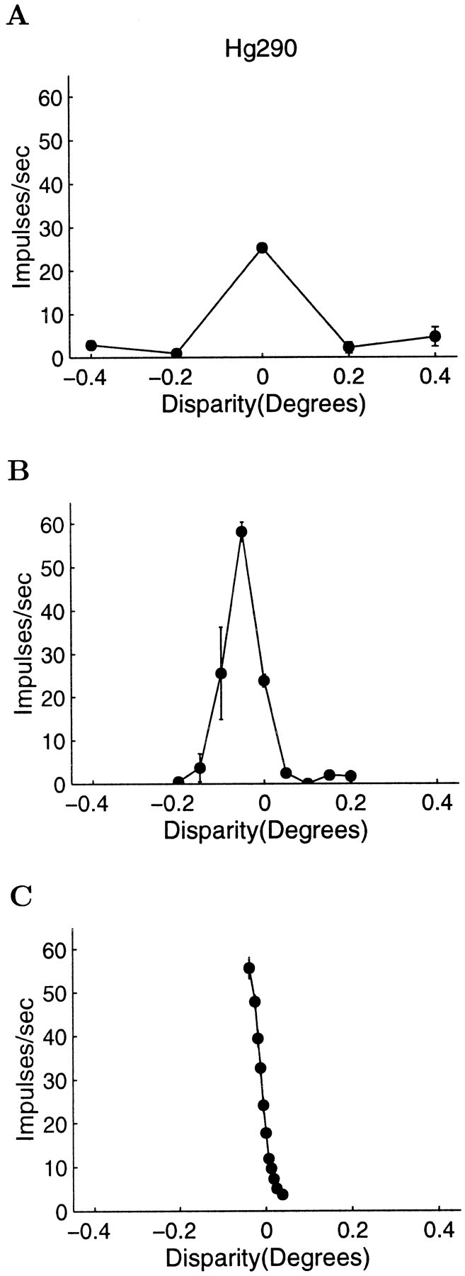
Example of the data collection protocol from a complex cell in monkey Hg. This is the same cell (Hg290) presented in Figure 1B. A, The disparity-tuning curve was initially coarsely sampled. B, If the cell appeared to be disparity-tuned, sample spacing was reduced until the steepest monotonic portion of the curve was found (C). In this case, the background reference disparity was set to zero. This threshold of the neuron for detecting differences in disparity was 0.75 arc min (see Fig. 3 for details of the calculation).

Implementation of neurometric functions and threshold estimation. For the purposes of this analysis, it is assumed that neural discrimination is based on the responses of two neurons with similar characteristics. The first of these is the recorded neuron that is responding to the disparity of the central patch. The second neuron is a theoretical construct with identical properties to the measured neuron but with a receptive field located in the stimulus surround. This will be referred to as the “orthoneuron.” The responses of the orthoneuron are derived by randomly selecting from the responses of the recorded neuron measured on trials when the disparity of the center and surround were the same. On a given trial, the firing rates of the neuron–orthoneuron pair are used to decide whether the central patch has a crossed or uncrossed disparity relative to the surround. This is illustrated in Figure 3A. This is closely related to the neuron–antineuron formulation of Britten et al. (1992), but it differs in critical ways, which are addressed in the Discussion.

Fig. 3.

A, Neurometric functions were calculated using a neuron–orthoneuron formulation. The top of the diagram represents the stimulus. The bottom left portion shows the disparity tuning of the neuron whose receptive field was matched to the center of the stimulus. The bottom rightportion shows the assumed disparity-tuning function of the orthoneuron. This is a theoretical neuron with identical response properties to the neuron, except that its receptive field is located in the surround portion of the stimulus. During the experiment, the surround has a constant disparity. Hence, the responses of the orthoneuron are assumed to correspond to the responses of the recorded neuron when presented with a center disparity of the same value as the surround disparity (in this case, 0.0°). The bottom left and bottom right tuning curves each have one data point highlighted by asolid symbol. The highlighted points correspond to the case when the disparity of the central patch is at a small crossed disparity (−0.006°) relative to the surround (0.0°). B, The spike distributions of the neuron at the current disparity and the orthoneuron at the disparity of the surround are compared to calculate an ROC curve. The area under the ROC curve gives the probability of successfully discriminating the disparity of the center (−0.006°) from the disparity of the surround (0°). C, This probability is calculated at a number of different stimulus levels to form a neurometric function. A cumulative Gaussian was fit to the data, and the SD, ς, of this curve was used as a measure of the neuronal discriminability. In this case the threshold is 0.012° or 0.72 arc min.

To estimate the discrimination performance of a neuron–orthoneuron pair, receiver operating characteristic (ROC) analysis (Green and Swets, 1966) was applied to the physiological data. For each measured disparity level, the ROC curve is constructed. The ROC curve is a two-dimensional plot of hit probability on the ordinate against false alarm probability on the abscissa. To calculate each pair of hits and false alarms, the spike count produced by the neuron is assessed against a criterion spike count. Here, the hit rate is defined as the probability of exceeding that criterion with a spike count randomly drawn from the responses of the measured neuron to the disparity present on that trial. The false alarm probability is the probability of exceeding the same criterion with a spike count drawn from the firing distribution of the orthoneuron: recall that the distribution for the orthoneuron is simply the responses of the neuron recorded on trials when the center and annulus had the same disparity. The entire ROC curve was calculated by sweeping the criterion count from 0 impulses to a value greater than the largest recorded spike count (Barlow et al., 1971). The area under each ROC was calculated. This corresponds to the probability that an ideal observer could discriminate the center and surround disparities on a given trial by processing the output of the neuron. This is illustrated in Figure3B.

These calculated probabilities were used to construct neurometric functions, which plot the neural discrimination performance as a function of disparity. An example of a neurometric function is shown in Figure 3C. Neural thresholds were calculated by fitting a cumulative Gaussian function to the neurometric function, by the same procedure that was used to fit the psychometric data. (This assumed that the percentage correct discrimination at each disparity followed a binomial distribution, and maximum likelihood was used to assess goodness of fit.) The SD of this Gaussian was taken to be a measure of the neural discrimination performance. Fitting was limited to points that lay on a monotonically increasing or decreasing portion of the tuning curve; 95% confidence limits for the fitted SD were calculated by a bootstrapping technique: the original firing distributions were resampled with replacement 1000 times, and a curve was fit to each simulated data set. Confidence limits on ratios of neuronal and psychophysical thresholds were calculated by calculating the ratio of thresholds for resampled neurometric and psychometric curves.

Measurement of other cell parameters. Cells were classified as simple or complex using the method of Cumming et al. (1999). The response to drifting gratings was subdivided into segments, whose duration corresponded to a single temporal period of the stimulus. Segments that contained a saccade were discarded. From the remaining segments, the ratio of the modulation at the temporal frequency of the stimulus (F1) to the mean firing rate (F0) was calculated. The cell was classified as complex when this F₁/F₀ ratio was <1.0 (Skottun et al., 1991). Orientation preference was assessed for the majority of units by measuring the response to bars moving backward and forward across the receptive field as a function of orientation. Typical response curves are shown in Figure4, A and B. The preferred orientation was taken to be the mean position of a fitted Gaussian (Fig. 4, legend). For some neurons, orientation tuning was also measured with drifting sinusoidal gratings, and a second measure of preferred orientation was estimated. The preferred orientation of the cell was calculated from the grating data when available and the bar data when not. The spatial frequency preference for grating stimuli was assessed in a similar manner for many units. Cell response was measured as a function of grating spatial frequency, and a Gaussian in log frequency was fit to the resulting curve. The preferred spatial frequency was taken to be the peak of this curve. Visual inspection revealed that the quality of fits was sufficiently good for an estimation of the peak frequency. Two examples of spatial frequency-tuning curve are shown in Figure 4, C and D. Ocular dominance was assessed quantitatively by measuring the monocular responses to drifting gratings of preferred orientation and spatial frequency for each eye separately and converting the firing rates to an ocular dominance index (similar to LeVay and Voigt (1988), without correction for spontaneous activity).

Fig. 4.

Examples of orientation-tuning and spatial frequency-tuning curves for two neurons. A and B show orientation-tuning curves for neurons Hg282 and Rb526, respectively. The abscissa shows the orientation of the bar stimulus in degrees. The ordinate shows mean firing rate in impulses per second. A Gaussian was fit to this data using an iterative curve-fitting procedure. The preferred orientation was taken to be the peak position of this curve. C and D show the spatial frequency-tuning curves for the same two cells. In each case, the abscissa shows the spatial frequency of the sinusoidal grating stimulus in cycles per degree. The ordinate shows the mean firing rate in impulses per second. A Gaussian in log spatial frequency was fit to this data, using an iterative curve-fitting procedure. The preferred spatial frequency was taken to be the mean position of this curve. Neuron Hg282 had a disparity threshold of 2.1 arc min, a preferred orientation of 1° clockwise from horizontal, and a peak spatial frequency of 1.7 cycles/°. Neuron Rb526 had a disparity threshold of 4.9 arc min, a preferred orientation of 128° clockwise from horizontal, and a peak spatial frequency of 2.4 cycles/°, and an ocular dominance index of 0.55.

RESULTS

Cell population parameters

In recordings from 232 neurons, 131 showed a significant effect of disparity on firing rate at a 5% level using a one-way ANOVA (97 of 163 in monkey Hg, 43 of 69 in monkey Rb). From this population of cells, simultaneous psychophysical and neuronal data were gathered from 18 cells in monkey Hg and 23 cells in monkey Rb. Neuronal discrimination data alone was gathered from a further nine cells in monkey Hg. These cells were selected from the larger population by two criteria. First, they had to be sufficiently well tuned for disparity to allow the construction of neurometric functions. A one-way ANOVA yielded a probability value of <0.01% for 92 cells. Second, isolation had to be maintained for long enough to record sufficient neural and psychometric data to estimate stereoacuity thresholds. Specifically, to be admitted to neurometric analysis, a minimum of 20 repetitions had to be gathered for at least seven different disparities. Where possible, more data were gathered, as in Figure 2C. It typically took 1–2 hrs to gather all data on a single cell.

Eighteen of seventy-five of the cells in which the response to sinusoidal gratings was measured were classified as simple in monkey Hg. Thirteen of forty-two of such cells in monkey Rb were categorized as simple. Of the cells in which neural discrimination was measured, 4 of 19 cells in monkey Hg and 4 of 14 cells in monkey Rb were classified as simple. The preferred spatial frequency of the cells from which neurometric functions were obtained varied from 0.6 to 6.5 cycles/°. The visual eccentricities at which these receptive fields were located are indicated in Figure 5. The preferred orientation of these cells varied continuously and evenly from horizontal to vertical (Fig. 6). The ocular dominance in the recorded cells varied from totally monocular to evenly balanced (see Fig. 9).

Fig. 5.

The calculated neurometric thresholds (degrees on the left ordinate and the equivalent in minutes of arc on the right ordinate) are plotted against the visual eccentricity of the stimulus center (degrees of visual angle on the abscissa). The threshold is expressed as the SD of the fitted cumulative Gaussian (see Fig. 3). Error bars are 95% confidence limits. Open andclosed symbols indicate data from monkeys Rb and Hg, respectively.

Fig. 6.

The calculated neurometric thresholds (degrees on the left ordinate and the equivalent in minutes of arc on the right ordinate) are plotted against preferred orientation (degrees rotation from horizontal on the abscissa) as assessed using either bar stimuli or sinusoidal gratings. Neural stereoacuity was good over the full range of preferred orientations. The two data points plotted withcircles indicate the example neurons plotted in Figure 4, A and B.

Fig. 9.

Plot of the calculated neurometric thresholds (degrees on the left ordinate and the equivalent in minutes of arc on the right ordinate) against the ocular dominance index of the cell (abscissa). An ocular dominance index of 0.5 indicates that the cell had evenly balanced inputs. Ocular dominance indices at the extremes of the distribution indicate that the cell was driven only by the contralateral or ipsilateral eye.

Neural discrimination data

Human psychophysical data suggests that stereoscopic depth thresholds rise as a function of visual eccentricity and the degree of deviation from the binocular horopter (pedestal disparity) (Blakemore, 1970; Rawlings and Shipley, 1969). The neural discrimination thresholds are presented as a function of visual eccentricity in Figure 5. There is no clear relationship between the neural discrimination threshold and eccentricity over the range 0.5–5°. Further analysis (not detailed here) also demonstrated that these neuronal thresholds were not well predicted by the pedestal disparity around which the neurometric threshold was calculated. The failure to observe a tight relationship between neuronal performance and eccentricity and pedestal disparity may be attributable to the heterogeneity of the cell population in V1 and the limited range of eccentricities explored. Also, any effect of eccentricity might be confounded with other parameters that are varying, such as the preferred spatial frequency, orientation, and patch size of the cell. We will return to this point after more detailed examination of the animal's psychophysical performance.

Figure 6 shows a plot of neurometric threshold against the preferred orientation for the 37 cells where both sets of information are available. There is no strong relationship between the preferred orientation of the receptive field and the neurometric threshold. This is intriguing, because most current models of cortical binocularity would predict that receptive fields with vertically elongated structure would support the highest stereoacuity.

Figure 7 plots the neurometric threshold against the effective horizontal frequency of the cell (the spatial frequency of a horizontal section through the preferred grating stimulus). This is calculated from the preferred orientation and spatial frequency of the cell. As the orientation, θ, departs from vertical, the horizontal period of the preferred stimulus changes with cos(θ). In these calculations, the peak orientation was estimated from the grating data when possible and the bar data when not. The measurements of neuronal discrimination with random dot stereograms only manipulate the horizontal disparity, regardless of the tuning preferences of the neuron under study. Hence, it is possible that the effective horizontal frequency, rather than stimulus spatial frequency of the neuron, might limit the neurometric threshold. However, the data show no tendency for the neurometric threshold to decrease as the effective horizontal frequency increases. Indeed, the three cells with the lowest values of horizontal frequency are among those with the lowest neurometric thresholds.

Fig. 7.

Plot of calculated neurometric thresholds (degrees on the left ordinate and the equivalent in minutes of arc on the right ordinate) against the stimulus preference of the neuron expressed as the effective horizontal spatial frequency. This was calculated from a combination of spatial frequency and orientation-tuning data (see Results). There is no tendency for the neurometric threshold to decrease as the effective horizontal frequency increases. Thecircles indicate data from the example cells in Figure4.

Several previous studies (Poggio et al., 1988) have suggested than only complex cells respond to the disparity in dynamic random dot stereograms. In agreement with this, we found that mean firing rates of simple cells in response to random dot stereograms were generally lower than those of complex cells. Despite the lower firing rates, some simple cells did produce good discrimination performance. Figure8 plots the neurometric threshold against the F₁/F₀ ratio. Although the absolute number of simple cells (where F₁/F₀ ≥ 1) is small, it is clear that two of the cells that are most sensitive to stereoscopic depth are actually simple in their spatial summation characteristics. As a whole, no difference was observed in the measured neurometric thresholds for simple or complex cells for either animal in this study.

Fig. 8.

Neurometric thresholds are plotted against the F₁/F₀ ratio. Typically cells are classified as complex if this ratio is <1. Although there is a majority of complex cells in the data set, there is no evidence to suggest that either type of cell is superior at discriminating horizontal disparity in the random dot stereograms.

Figure 9 plots the neurometric threshold as a function of the ocular dominance index. This is defined as

$$ODI=\frac{I}{I+C},$$

where I is response to a monocular drifting grating of the preferred orientation and spatial frequency of the cell presented to the ipsilateral eye alone, and C is the response to a grating presented to the contralateral eye alone. This produces a scale that varies continuously from 0 to 1 similar to that used by LeVay and Voigt (1988), rather than the original seven-point scale used byHubel and Wiesel (1968). Unlike the scale used by LeVay and Voigt (1988), we did not subtract spontaneous activity before calculating this ratio, because valid measurements of spontaneous activity were not available for all neurons in this data set. This means that the scale used here is slightly compressed at the extreme values compared with the scale used by LeVay and Voigt (1988). Values near 0 and 1 on this continuous scale correspond to “purely monocular” neurons (classes 1 and 7 on the original scale), whereas values near 0.5 correspond to neurons driven equally well by either eye (class 4, “binocular neurons,” on the original scale). Although there is a weak predominance of neurons with indices near 0.5, this appears primarily to reflect a difference between the two monkeys, rather than a systematic relationship with neurometric threshold. This is consistent with both LeVay and Voigt (1988), who found no relationship between ocular dominance and disparity selectivity in cat areas 17 and 18, andSmith et al. (1997), who also failed to find any relationship between these parameters for complex cells in macaque V1.

Comparison of neurometric and psychometric thresholds

Figure 10 plots the simultaneous psychometric threshold as a function of the neurometric threshold. The best psychometric thresholds for monkey Hg are <1.0 arc min, and the lowest threshold is ∼0.2 arc min. Thresholds in monkey Rb were generally higher, and the best threshold found was 1.2 arc min. The relationship between neurometric and psychometric performance is presented as the ratio of the neurometric to the psychometric threshold (the N:P ratio). When this is greater than one, the performance of the neuron is worse than the performance of the animal as a whole. When the ratio is less than one, the performance of the neuron is better than the monkey's behavior. The histogram in Figure 10 shows the distribution of this N:P ratio, summarized for both monkeys. The (geometric) mean N:P ratio was 2.51 for 18 cells in monkey Hg and was 1.21 for the 23 cells recorded in monkey Rb. Hence, the response of the neurons was generally worse than the performance of the animal as a whole. However, in one case in monkey Hg and in eight cases in monkey Rb the neuronal stereoacuity was better than the performance of the animal as a whole. There was no discernible relationship between the N:P ratio and the preferred spatial frequency or orientation of the cell, F₁/F₀ ratio, or the stimulus pedestal disparity. The mean N:P ratio across both animals was 1.67, superficially similar to previous studies in which psychophysical and neuronal performance was measured simultaneously (for motion discrimination in area MT): 1.19 in Britten et al. (1992), and 1.50 inCroner and Albright (1999).

Fig. 10.

The simultaneous psychometric threshold is plotted against the neurometric threshold. The diagonal lineindicates the locus of points where both thresholds are the same. Points below this line indicate experiments in which the neurometric threshold was greater than the psychometric threshold. The histogram shows the distribution of the N:P threshold ratio. The neuronal thresholds are on average slightly higher than the psychometric thresholds.

Revised determination of psychophysical thresholds

One possible source of error with this comparison of neuronal and behavioral thresholds arises if the monkey had not been performing the task as well as possible. In particular, the stimulus levels in each experiment were determined by the disparity-tuning curve of the recorded neuron. If these levels are widely spaced relative to the animal's psychophysical ability, the monkey may not be motivated to perform well on the near threshold trials, as a reasonable rate of rewards can be achieved just from the “easy” trials alone. The structured analysis of variance presented by Britten et al. (1992)suggests that such a factor may have influenced behavior in that study: even after stimulus variables had been taken into account, there was a small but significant correlation between neural threshold and psychometric threshold. To evaluate this possibility thoroughly in our data, the psychometric functions were all remeasured after the neuronal recordings were complete (these new psychophysical thresholds will be termed the “subsequent thresholds”). All stimulus parameters, except the range of disparities, were identical to those presented during the original recording.

The effect of an inappropriate choice of stimulus levels on psychophysical performance is demonstrated for our data in Figure11, A and B. Figure 11A shows the neurometric function, which is clearly well sampled and well fit by the cumulative Gaussian (the solid line). The circular symbols and solid curve on Figure 11B show the simultaneously recorded psychometric function. Performance is consistently close to 100% at all disparities, apart from the center point at which one would expect chance behavior. However, the animal never successfully reaches 100% correct because of occasional errors. Consequently, the best curve fit drastically overestimates the threshold. The square symbols and dashed curve of Figure 11B show the outcome of measuring the psychometric function with a more appropriate stimulus range. The cumulative Gaussian now fits the data considerably better, and the estimate of the psychophysical threshold is much lower.

Fig. 11.

A, Neurometric function for calculation of neuronal threshold. Sampling was optimized for this calculation. The measured neurometric threshold was 5.35 arc min. B, The circles and solid curve show results from the simultaneous recording of behavior. The stimulus spacing for this task was considerably greater than was necessary. The monkey fails to consistently maintain 100% performance at the suprathreshold stimulus levels. This causes the curve fitting to overestimate the threshold to be 5.32 arc min. The squaresand dashed curve depict subsequently measured psychophysical behavior for a random dot stereogram with identical stimulus parameters but a more appropriate disparity range. The measured behavioral threshold was then considerably smaller at 0.35 arc min. C, A second neurometric function for calculation of neuronal threshold. Again, sampling was optimized for this calculation. The neurometric threshold was 2.12 arc min. D, The stimulus spacing for the simultaneous psychophysical task was considerably greater than was necessary (circles, solid curve), and the threshold is estimated to be 1.21 arc min. However, in this case, the curve is a good fit to the data. When behavior was remeasured with more appropriate stimulus values (squares, dashed line), the measured behavioral threshold was also considerably smaller at 0.30 arc min.

One potential approach to this phenomenon would be to argue that the poor fit of the Gaussian curve to the behavioral data should result in the elimination of this data. There are two problems with this. First, this might selectively remove units in which the N:P ratio was high. Second, psychometric functions in which the stimulus levels were inappropriate cannot always be identified by a poor curve fit. Figure11, C and D, shows a example of this type. Although the simultaneously recorded responses are well described by a cumulative Gaussian, the threshold was considerably smaller when behavior was remeasured with a different stimulus range. Again, circular symbols and the solid line represent simultaneous behavior, and square symbols and the dashed line represent subsequently measured behavior. It is interesting to note that, in both the simultaneous and subsequent cases, the animal's reward rate is approximately the same, despite the much harder task it faces in the subsequent conditions. This suggests that the animal's motivation may be decreasing once a certain reward rate is achieved.

Figure 12 summarizes the relationship between the simultaneous and subsequent psychometric thresholds for depth discrimination in random dot stereograms, in the same format as Figure 10. The plot on the left shows the simultaneous thresholds plotted against the subsequent thresholds, and the histogram on the right shows the distribution of the ratio of these two psychophysical thresholds averaged over data from both animals. It is particularly notable that the ratio for monkey Rb is always less than one, indicating that the subsequently recorded threshold was lower in every single case. The average improvement in the measured stereoacuity was a factor of 1.8 for monkey Hg and a factor of 3.4 for monkey Rb.

Fig. 12.

The subsequent psychometric threshold is plotted as a function of the simultaneous psychometric threshold. For each point on the graph, the stimuli were identical apart from the disparities used. The diagonal line indicates the locus of points where both thresholds are the same. Points above this line indicate experiments where the simultaneous threshold was greater than the subsequent threshold. The subsequent threshold is lower than the simultaneous threshold in every case for monkey Rb and for most measurements in monkey Hg. The histogram shows the distribution of the simultaneous:subsequent threshold ratio.

The misestimation of the monkey's behavioral capabilities under simultaneous recording conditions will necessarily have affected the comparison of neuronal and behavioral acuity. Figure13 plots the N:P ratio after remeasurement of the psychometric functions. This plot also includes ratios calculated from nine cells in monkey Hg, for which simultaneous psychophysics had not originally been recorded. Figure 13 shows that almost all V1 neurons perform worse than the observer as a whole. Data pooled from both monkeys shows that individual neurons perform on average 4.1 times more poorly than the observer as a whole. Only two neurons in each monkey outperform the observer. These four neurons yielded thresholds ∼1.6 times lower than the corresponding psychometric thresholds. One striking difference between the data in Figure 13 and Figure 10 is the degree of correlation between psychometric and neurometric thresholds. Significant correlation is evident only for the simultaneously recorded psychophysics. Such a correlation could arise if differences in the stimuli used have similar influences on neuronal and psychophysical performance. However, the lack of correlation for the subsequent psychophysics argues against this. Therefore, it seems likely that the correlation in Figure 10arises because the disparity range chosen to measure the neurometric threshold has an influence on the psychophysical performance.

Fig. 13.

The subsequent psychometric threshold is plotted as a function of the neurometric threshold. Again the diagonal line indicates the locus of points where both thresholds are the same, and the N:P ratio is one. Points below this line indicate experiments where the neurometric threshold was greater than the psychometric threshold. For both monkey Hg and monkey Rb, most points are below this line. The histogram shows the distribution of the N:P ratio collapsed over both animals. The mean N:P ratio is slightly >4, indicating that on average the observer performs approximately four times better than the V1 neurons in this sample.

Britten et al. (1992) also raised the possibility that psychophysical performance in their experiments might have been suboptimal. They argued that this was unlikely because the macaque thresholds were similar to those for human observers and that the macaques' performance was highly reliable. However, because their data show a large scatter in psychophysical threshold, it is difficult to be sure that this argument holds in general, and their structured ANOVA suggests that there was some effect of this type. Because they did not remeasure psychophysical thresholds, it is hard to evaluate the magnitude of any effect, but indirect arguments suggest that the effect is probably smaller in their data than the effect we show here. For example, in our data, the choice of points for measuring the psychometric function influences the monkeys' behavior so that there is a strong correlation between neurometric threshold and psychometric threshold, whereas in Figure 10 of Britten et al. (1992), no such correlation is apparent.

Several features of the subsequent psychophysical thresholds suggest the animals are performing close to the limits of their performance under these circumstances. Figure 14shows a plot of these thresholds against eccentricity and pedestal disparity. This plot shows that the highest thresholds were found when the eccentricity or pedestal disparity were large. Although the effect of these parameters in these two macaque monkeys is slight, the outcome is in agreement with earlier results from the human psychophysical literature (Rawlings and Shipley, 1969; Blakemore, 1970).

Fig. 14.

The revised measurements of psychometric threshold for behavioral depth discrimination are plotted as a function of eccentricity. Solid symbols show cases in which the absolute disparity of the pedestal (the disparity of the surround patch) was within 0.1° of the binocular fixation point, whereasopen symbols show cases in which the pedestal disparity was larger. Thresholds were generally best when both the pedestal disparity and the eccentricity were small. The gray bar indicates the range of human performance for four observers as measured using similar stimuli at an eccentricity of 4.0°.

For human observers, stereoacuity can be as small as a few arc seconds, but only for foveally presented stimuli of high contrast (Westheimer, 1979; Woo and Sillanpaa, 1979; McKee, 1983). We measured thresholds in four human subjects with our random dot stimuli. The mean threshold at an eccentricity of 4° was 0.87 min arc (±0.32′, SD), very similar to the performance of the two monkeys (Figure 14) and previously published human thresholds at such eccentricities (Ogle, 1956; Fendick and Westheimer, 1983; Westheimer and Truong, 1988; Siderov and Harwerth, 1995). Previous investigations have suggested that macaque stereoacuity with random dot stereograms is poorer than for humans (Harwerth and Boltz, 1979), but is comparable when difference of Gaussian stimuli are used (Harwerth et al., 1995). The data presented here suggests that under optimal conditions, macaque stereoacuity with random dot stereograms is as good as that of humans.

Relative or absolute disparity?—the effect of the background

There is another perspective from which the comparison made here between neuronal and behavioral performance could be deemed inappropriate: the surrounding annulus of random dots may have quite different effects on neurometric and psychometric performance. The center part of the random dot stimulus was matched to the receptive field size, and it has been assumed up until this point that the disparity of the center alone is responsible for the stimulus-related variation in recorded firing rates. Indeed Cumming and Parker (1999)have demonstrated that the disparity of annular surround regions of the sort used here has no effect on the mean firing rates of disparity-selective neurons in V1. However, human stereoacuity is diminished by an order of magnitude in the absence of a nearby disparity reference (Westheimer, 1979; McKee and Levi, 1987). Hence, if the surround region of the random dot stereogram were to be removed, one predicts that the monkey's behavior might suffer, but neural performance in V1 should remain constant.

To assess the effect of the background annulus, psychophysical stereoacuity was remeasured with stimuli identical to those used previously, except that the annular surround was altered. In the first condition, the surround consisted of binocularly uncorrelated random dots. This provides a visible surround area, but it is impossible to assign a consistent binocular disparity to the field of dots forming the surround. In the second condition, the surround was absent altogether. In both these conditions, it is assumed that the animal now makes decisions about the depth of the central patch of dots relative to the disparity of the fixation marker, which was always binocularly visible. The animals' decisions were rewarded on this basis. Figure15 shows the effect on psychophysical thresholds for two cases, one for each monkey. In each case, behavioral thresholds increased by a factor of 10 when the surround is absent or uncorrelated, consistent with the findings of Westheimer (1979), who concluded that “good stereoacuity has as a prerequisite the simultaneous unencumbered view of at least a pair of targets” (p 591). In fact, there are two visible targets even when the annular surround is absent, because the fixation marker is visible throughout the trial. Presumably the distance between the fixation marker and the patch of dots limits the usefulness of the relative disparity signal, as would happen if the visual system only determines relative disparities locally.

Fig. 15.

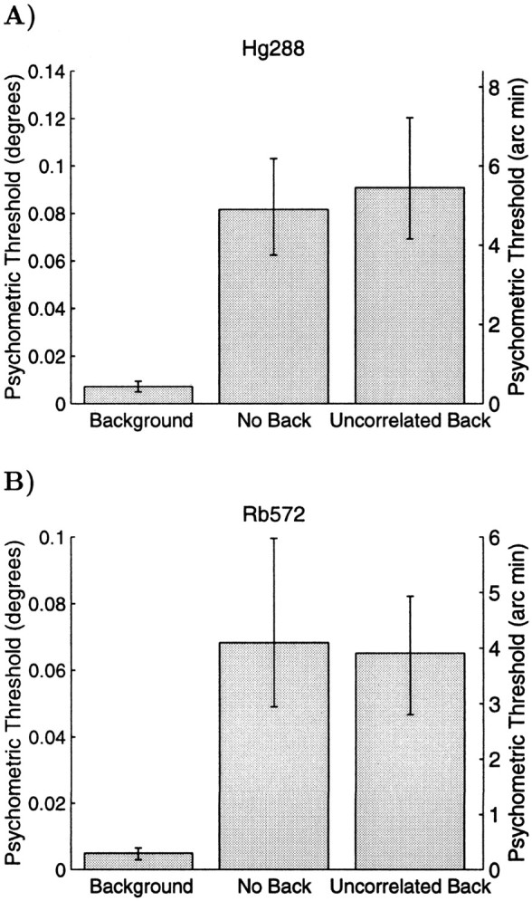
Example psychometric thresholds for depth discrimination in three conditions. When the background is present, the threshold is low. When the background is uncorrelated or absent, the psychometric thresholds are an order of magnitude higher. This is shown for one stimulus configuration in monkey Hg (A) and one in monkey Rb (B).

In the absence of a surround, animals are forced to make judgments relative to the fixation marker, which has disparity of 0°. Therefore it is only meaningful to compare neurometric and psychometric thresholds for configurations in which the stimulus preferences of the neuron had allowed us to measure thresholds around a pedestal disparity of 0°. Figure 16 shows the N:P ratio with and without the surround region for all eight of these cases. The psychometric threshold changes by an order of magnitude when the surround is removed, and so the N:P ratio changes in the same way. As a consequence, individual neurons are frequently more sensitive than the observer as a whole (five of eight cases). This is difficult to reconcile with models of the psychophysical threshold based on the lower envelope principle (Parker and Newsome, 1998). If there are neurons that outperform the psychophysical observer, how is it that the observer cannot access the information being signaled by these neurons? There are two possible answers.

Fig. 16.

The N:P ratio for the condition with no background is plotted on the ordinate against the N:P ratio for the condition with the background present on the abscissa, for the eight cases in which the neurometric function had been measured around zero disparity. For each point, the measurement of neuronal performance was the same for both ratios. The psychophysical component of each ratio consists of the subsequently measured thresholds in the presence or absence of a zero disparity background patch. All of the data points fall below the diagonal line, which indicates that the psychophysical performance was always worse in the absence of a background. Thedashed line shows the mean change in the N:P ratio, which falls by a factor of 10.8 (geometric mean) when the background is absent.

First, it is possible that removing the surround annulus might actually have an effect on the firing patterns of V1 neurons. However, becauseCumming and Parker (1999) showed that the mean firing rate depends only on absolute disparity, this effect would have to be exclusively manifest as a reduction of the variance of the firing rate. A reduction in the variance of neuronal discharge with no change in mean firing patterns would create an improvement in neuronal discrimination performance (cf. Croner and Albright, 1999). However, the variance would have to change by a factor of ∼100 to explain the 10-fold change in psychophysical threshold, which makes this explanation unlikely. Nonetheless, to demonstrate with certainty that single V1 neurons systematically outperform the observer on an absolute disparity task, it would be necessary to repeat both neurometric and psychometric measurements without an effective annulus.

Second, the psychophysical observation that a simultaneous visual reference is required for best stereoacuity is usually attributed to convergence instability (Foley, 1976; Westheimer, 1979; McKee et al., 1990). If vergence eye position is unstable, the absolute disparity of the stimulus changes on the retina. However, because V1 neurons signal absolute disparity (Cumming and Parker, 1999), such fluctuations in absolute disparity should also limit the neurometric threshold as measured here. (Recall that the comparison of neuronal response distributions is based on data collected from the response of a single neuron on independent trials, not on the simultaneous recording of two neurons.) This argument forces us to conclude that true vergence variability by itself is not an explanation for the superiority of V1 neurons over psychophysical performance when the annular surround is absent. It may be that the observers' uncertainty about vergence eye position limits the ability to interpret signals related to absolute disparity. On this view, the monkeys' true vergence control is better than their visual system is prepared to assume. In this case, the animals may actually exploit the signals in V1 neurons directly, but they simply set a much higher statistical criterion for acknowledging a change in firing rate, if they cannot be certain whether the change in firing is caused by movements of their eyes or a change in the stimulus.

Finally, it may be that the lower envelope principle fails simply because observers do not have direct access to signals from V1 neurons for this task. Because there is some real variation because of vergence that affects the firing of all neurons selective for absolute disparity, the difference in firing between an appropriate pair of neurons recorded simultaneously will not be affected by changes in vergence. This difference signal appears to be used psychophysically and would produce still lower neurometric thresholds than those reported here. If such a differencing operation is part of neuronal circuitry, then it presumably occurs beyond the striate cortex, where neurons may consequently achieve better stereoacuity. The best psychophysical performance would then derive from monitoring the activity of such neurons.

DISCUSSION

ROC analysis was used to estimate the ability of neurons to discriminate the disparity of the center of a dynamic random dot stereogram relative to the disparity of the surround. There was no clear relationship between the neurometric threshold and preferred orientation, preferred spatial frequency, ocular dominance, or simple/complex classification. The identification of a neuron with good discrimination performance for horizontal disparity appears to be a poor predictor of other response properties. However, it is important to understand that because we only performed neurometric analysis on neurons that showed good disparity tuning, the sample of neurons analyzed here will be biased by this criterion. It remains possible that one could identify subgroups of neurons in striate cortex that are more likely to yield good discrimination performance. For example, although our data show that cells preferring horizontal orientations are able to support very good discrimination performance, it does not necessarily mean that in general cells preferring horizontal orientations always produce performance as good as those preferring vertical orientations.

The neurometric thresholds were compared with the psychophysical thresholds of the same animals in response to the same stimuli. The animals were able to use the relative disparity between center and surround to perform the psychophysical task, so this comparison addresses the question of whether the signals about absolute disparity in primate V1 are sufficiently precise to support psychophysical judgments of relative disparity. The ratio of stereoscopic acuity for the neuron relative to the animal's behavior measured simultaneously (N:P ratio) was found to be 1.67 on average. Neuronal performance was on average only slightly poorer than behavioral.

However, these simultaneous measurements of psychophysical performance were suboptimal because of the choice of stimulus levels. If the neuronal response function has a relatively gentle slope, widely spaced stimuli will be needed for the construction of a neurometric function, but these stimuli are then inappropriately spaced for measurement of a psychometric function. When the stimulus levels are too far apart, the animal's motivation may decrease. Remeasurement of psychophysical performance with more appropriate stimulus levels yielded thresholds that were improved by a factor of more than two. This yielded a revised N:P ratio of 4.1. This highlights the importance of ensuring that psychophysical performance is optimal before making comparisons with neuronal measurements.

For a motion discrimination task, Britten et al. (1992) examined the performance of motion-selective cells in macaque visual area V5 (MT) and found an average N:P ratio of 1.19. Croner and Albright (1999)reported finding a similar value of 1.5. Our mean N:P ratio of 4.1 was significantly higher than both these values (one-tailed t test on log ratio; p ≤ 0.001).

Orthoneuron and antineuron

One reason why the average N:P ratio found by Britten et al. (1992) is smaller than our estimate arises from their formulation of the neuronal task. In both studies, the psychophysical procedures were formally equivalent (Figure 17). ForBritten et al. (1992), the behaving monkey was presented with a single sample of visual motion for a direction judgment, and made a binary forced-choice decision. In our case, a single stereogram was presented, and a binary forced-choice judgment about depth was reported. However, there are differences in the calculation of neuronal thresholds.Britten et al. (1992) analyzed the responses of a theoretical neuron–antineuron pair to estimate thresholds. This compared the distribution of responses at a given stimulus level (% correlated dots) with the distribution of responses to the same stimulus level when it moved in the opposite direction. This second response is taken to represent the signal from a theoretical “antineuron” with identical properties, except that it has the opposite direction preference. Consistent with many models of motion detection, the difference between these two neuronal signals was used to construct the neurometric function.

Fig. 17.

Comparison of the neurometric and psychometric measurements made here and in Britten et al. (1992). In our study, the observer judges the disparity of the center part of the stimulus relative to the surround, after a single stimulus presentation. The observers in Britten et al. (1992) also saw a single stimulus presentation and judged the direction of the signal dots (solid arrows and dots) in the presence of noise dots (open arrows and dots). Thus the two psychophysical tasks are formally equivalent (single interval binary forced choice). However, the neurometric analyses are different. Our neurometric analysis comprises one neuron that measures the center disparity and a theoretical orthoneuron that measures the surround. This compares the firing of the neuron to a nonzero disparity with the firing when the disparity was zero. Britten et al. (1992) compared responses of each neuron with a theoretical antineuron, (a neuron with opposite direction selectivity). This compares the firing of the neuron to one signal with the firing to a signal of the same strength but of opposite sign. The signal difference between the two stimuli under comparison is twice as large for the neuron–antineuron formulation as for the neuron–orthoneuron formulation. Depending on the shape of the tuning curve, estimates of neurometric thresholds can be up to a factor of two smaller, even when the calculations are performed on identical tuning curves.

Our analysis also uses the difference between two response distributions, but the distributions used are those in response to a given stimulus level and those to zero signal (when the center disparity equals that of the surround). The difference in the stimuli here is only half that used in a neuron–antineuron formulation, so identical tuning curves yield neurometric thresholds up to twice as large. We have confirmed this by recalculating our neurometric thresholds using a neuron–antineuron comparison, and the neurometric thresholds were smaller by a factor of 2.08 (geometric mean ratio). Thus, for comparison with the N:P ratios reported by Britten et al. (1992), the summary ratio of 4.11 shown in Figure 13 should be reduced to 1.97, which makes the apparent gap between the two studies much less severe.

The main reason why we used the neuron–orthoneuron formulation is that this makes use of neural signals relating to the surround portion of the stimulus. We are confident that the psychophysical observers actually rely on the disparity of the surround because their performance falls dramatically when it is not present. The neuron–orthoneuron formulation measures the information which is implicitly available about the relative disparity between center and surround.

When there is no surround (Figure 16), the neuron–orthoneuron formulation is less appropriate. If we then use the neuron–antineuron formulation to calculate neurometric thresholds, the N:P ratio is halved. When this adjustment is applied to the data in Figure 16, seven of eight neurons outperform the psychophysical observer, and the geometric mean of the N:P ratio is 0.58.

In summary, there are two factors that lead to larger N:P ratios here than reported by Britten et al. (1992): (1) their method of calculating the neurometric threshold produces lower values than our method, even if applied to the same tuning curve, and (2) the use of simultaneous psychophysical recording may result in an underestimate of psychophysical performance. Taking these two factors into account, it seems that the mean N:P ratio for disparity discrimination in V1 is similar to that for direction discrimination in MT. Despite the lack of specialization in V1 for disparity processing, neuronal discrimination performance is as good as neurons in specialized extrastriate areas. Contrary to suggestions based on qualitative comparisons of neuronal and behavioral data (Westheimer, 1979; Poggio and Poggio, 1984), it appears that the activity of only a few V1 neurons may be sufficient to explain psychophysical stereoacuities. Hence, even if their properties do not tally with perceptual phenomena (Cumming and Parker, 1997, 1999;Parker et al., 2000), they must be considered serious candidates for carrying the horizontal disparity signal used for stereopsis.

How appropriate is the N:P comparison?

However carefully the N:P ratio for single neurons may be evaluated, there are still numerous ways in which the mean N:P ratio could be biased in this type of experiment. First, it is potentially unfair to compare average N:P ratios, given that the primary visual cortex contains a heterogeneous population of cells and is not specialized for stereopsis. Hence, only units that were suitably tuned for this type of analysis were selected. A different selection criterion, in which less sensitive neurons were included, would necessarily inflate the mean N:P ratio upwards. Second, although the size and position of the random dot stereogram were optimized to drive the unit, it is always possible that adjusting some other stimulus parameter might improve neuronal performance. Third, the dynamic random dot stimuli used in this study are broadband in orientation, and temporal and spatial frequency content. Given the widespread assumption that V1 cells act as spatial filters, this stimulus should drive all V1 cells well. However, there may be parts of the stimulus spectrum that do not excite the particular cell under study but nonetheless provide the psychophysical observer with information.

The temporal duration of the stimulus must also be considered. The calculation of the neurometric function utilizes all the spike information from the stimulus duration of 2 sec. However, the animal's psychophysical decision process may not optimally integrate information over the whole stimulus period. Like Britten et al. (1992), we recomputed neurometric thresholds using different durations for a sample of cells and examined the effect of duration on psychophysical performance. Both neurometric and psychometric performance improve systematically with duration right out to the 2 sec duration used here, but further work is required to establish whether or not there are systematic changes in the N:P ratio.

Uncertainty and the effect of the surround

Details of exactly how the psychophysical task is specified may dramatically affect the N:P comparison. When the psychophysical behavior was remeasured with no useful disparity signal from the surround portion of the stereogram, thresholds increased by an order of magnitude. Our previous work indicates that neuronal thresholds would not be expected to change, because the surround is outside the receptive field (Cumming and Parker, 1999). Under these circumstances, it appears that the N:P ratio for disparity discrimination in V1 is substantially lower (i.e. better neuronal performance) than that for direction discrimination in MT.

The fact that neurometric thresholds are frequently lower that psychometric thresholds in this situation suggests that the elevated psychophysical thresholds cannot simply be attributed to fluctuations in vergence eye position, because these would place the same limit on neuronal performance. As an alternative, we suggest that the animals' intrinsic uncertainty (Pelli, 1985) about vergence position is greater than the true variation in vergence would warrant. Thus, even when a stimulus change produces a discriminable change in neural firing of a V1 neuron in an absolute disparity task, the animal does not know whether or not this is the result only of a change in vergence position. Any circumstances that increases stimulus uncertainty (in Pelli's meaning of the term) will raise the psychophysical threshold relative to the performance of the underlying mechanisms.

REFERENCES

- 1.Barlow H, Levick W, Yoon M (1971) Responses to single quanta of light in retinal ganglion cells of the cat. Vision Res [Suppl]:87–101. [DOI] [PubMed]
- 2.Barlow H, Kaushal T, Hawken M, Parker AJ. Human contrast discrimination and the threshold of cortical neurons. J Opt Soc Am A. 1987;4:2366–2371. doi: 10.1364/josaa.4.002366. [DOI] [PubMed] [Google Scholar]
- 3.Blakemore C. The range and scope of binocular depth discrimination. J Physiol (Lond) 1970;211:599–622. doi: 10.1113/jphysiol.1970.sp009296. [DOI] [PMC free article] [PubMed] [Google Scholar]
- 4.Bradley A, Skottun B, Ohzawa I, Sclar G, Freeman R. Visual orientation and spatial frequency discrimination: a comparison of single cells and behaviour. J Neurophysiol. 1987;57:755–772. doi: 10.1152/jn.1987.57.3.755. [DOI] [PubMed] [Google Scholar]
- 5.Britten KH, Shadlen MN, Newsome WT, Movshon JA. The analysis of visual motion: a comparison of neuronal and psychophysical performance. J Neurosci. 1992;12:4745–4765. doi: 10.1523/JNEUROSCI.12-12-04745.1992. [DOI] [PMC free article] [PubMed] [Google Scholar]
- 6.Croner LJ, Albright TD. Segmentation by color influences responses of motion-sensitive neurons in the cortical middle temporal visual area. J Neurosci. 1999;19:3935–3951. doi: 10.1523/JNEUROSCI.19-10-03935.1999. [DOI] [PMC free article] [PubMed] [Google Scholar]
- 7.Cumming BG, Parker AJ. Responses of primary visual cortical neurons to binocular disparity without depth perception. Nature. 1997;389:280–282. doi: 10.1038/38487. [DOI] [PubMed] [Google Scholar]
- 8.Cumming BG, Parker AJ. Binocular neurons in V1 of awake monkeys are selective for absolute, not relative disparity. J Neurosci. 1999;19:1981–2088. doi: 10.1523/JNEUROSCI.19-13-05602.1999. [DOI] [PMC free article] [PubMed] [Google Scholar]
- 9.Cumming BG, Thomas OM, Parker AJ, Hawken MJ. Classification of simple and complex cells in (V1) of the awake monkey. Soc Neurosci Abstr. 1999;25:1548. [Google Scholar]
- 10.Fendick M, Westheimer G. Effects of practice and the separation of test targets on foveal and peripheral stereoacuity. Vision Res. 1983;23:145–150. doi: 10.1016/0042-6989(83)90137-2. [DOI] [PubMed] [Google Scholar]
- 11.Foley JM. Successive stereo and vernier position discrimination as a function of dark interval duration. Vision Res. 1976;16:1269–1273. doi: 10.1016/0042-6989(76)90052-3. [DOI] [PubMed] [Google Scholar]
- 12.Geisler WS, Albrecht DG. Visual cortex neurons in monkeys and cats: detection, discrimination and identification. Vis Neurosci. 1997;14:897–919. doi: 10.1017/s0952523800011627. [DOI] [PubMed] [Google Scholar]
- 13.Green D, Swets J. Signal detection: theory and psychophysics. New York; Wiley: 1966. [Google Scholar]
- 14.Harwerth RS, Boltz RL. Stereopsis in monkeys using random dot stereograms: the effect of viewing duration. Vision Res. 1979;19:985–991. doi: 10.1016/0042-6989(79)90223-2. [DOI] [PubMed] [Google Scholar]
- 15.Harwerth RS, Smith EL, Siderov J. Behavioural studies of local stereopsis and disparity vergence in monkeys. Vision Res. 1995;35:1775–1770. doi: 10.1016/0042-6989(94)00256-l. [DOI] [PubMed] [Google Scholar]
- 16.Hawken MJ, Parker AJ. Detection and discrimination mechanisms in the striate cortex of the old-world monkey. In: Blakemore C, editor. Vision: coding and efficiency. Cambridge UP; Cambridge, UK: 1990. pp. 103–116. [Google Scholar]
- 17.Hubel D, Wiesel T. Receptive fields and functional architecture of monkey striate cortex. J Physiol (Lond) 1968;195:215–243. doi: 10.1113/jphysiol.1968.sp008455. [DOI] [PMC free article] [PubMed] [Google Scholar]
- 18.LeVay S, Voigt T. Ocular dominance and disparity coding in the cat visual cortex. Vis Neurosci. 1988;1:395–414. doi: 10.1017/s0952523800004168. [DOI] [PubMed] [Google Scholar]
- 19.McKee SP. The spatial requirements for fine stereoacuity. Vision Res. 1983;23:191–198. doi: 10.1016/0042-6989(83)90142-6. [DOI] [PubMed] [Google Scholar]
- 20.McKee SP, Levi DM. Dichoptic hyperacuity: the precision of nonius alignment. J Opt Soc Am. 1987;4:1104–1108. doi: 10.1364/josaa.4.001104. [DOI] [PubMed] [Google Scholar]
- 21.McKee SP, Welch L, Taylor DG, Browne SF. Finding the common bond: stereoacuity and other hyperacuities. Vision Res. 1990;30:879–891. doi: 10.1016/0042-6989(90)90056-q. [DOI] [PubMed] [Google Scholar]
- 22.Merrill EG, Ainsworth A. Glass-coated platinum-plated tungsten electrodes. Med Biol Eng. 1972;10:662–672. doi: 10.1007/BF02476084. [DOI] [PubMed] [Google Scholar]
- 23.Ogle K. Stereoscopic acuity and the role of convergence. J Opt Soc Am. 1956;46:269–273. [Google Scholar]
- 24.Parker AJ, Hawken MJ. Capabilities of monkey cortical cells in spatial resolution tasks. J Opt Soc Am. 1985;2:1101–1114. doi: 10.1364/josaa.2.001101. [DOI] [PubMed] [Google Scholar]
- 25.Parker AJ, Newsome WT. Sense and the single neuron: probing the physiology of perception. Annu Rev Neurosci. 1998;21:227–277. doi: 10.1146/annurev.neuro.21.1.227. [DOI] [PubMed] [Google Scholar]
- 26.Parker AJ, Cumming BG, Dodd JV. Binocular neurons and the perception of depth. In: Gazzaniga MS, editor. The new cognitive neurosciences. MIT; Boston: 2000. pp. 263–277. [Google Scholar]
- 27.Pelli D. Uncertainty explains many aspects of visual contrast detection and discrimination. J Opt Soc Am. 1985;2:1508–1531. doi: 10.1364/josaa.2.001508. [DOI] [PubMed] [Google Scholar]
- 28.Poggio GF, Poggio T. The analysis of stereopsis. Annu Rev Neurosci. 1984;7:379–412. doi: 10.1146/annurev.ne.07.030184.002115. [DOI] [PubMed] [Google Scholar]
- 29.Poggio G, Gonzalez F, Krause F. Stereoscopic mechanisms in monkey visual cortex: binocular correlation and disparity selectivity. J Neurosci. 1988;8:4531–4550. doi: 10.1523/JNEUROSCI.08-12-04531.1988. [DOI] [PMC free article] [PubMed] [Google Scholar]
- 30.Rawlings S, Shipley T. Stereoscopic acuity and horizontal angular distance from fixation. J Opt Soc Am. 1969;59:991–993. doi: 10.1364/josa.59.000991. [DOI] [PubMed] [Google Scholar]
- 31.Shadlen MN, Britten KH, Newsome WT, Movshon JA. A computational analysis of the relationship between neuronal and behavioural responses to visual motion. J Neurosci. 1996;16:1486–1510. doi: 10.1523/JNEUROSCI.16-04-01486.1996. [DOI] [PMC free article] [PubMed] [Google Scholar]
- 32.Siderov J, Harwerth R. Stereopsis, spatial frequency and retinal eccentricity. Vision Res. 1995;35:2329–2337. doi: 10.1016/0042-6989(94)00307-8. [DOI] [PubMed] [Google Scholar]
- 33.Skottun B, DeValois R, Grosof D, Movshon J, Albrecht D, Bonds A. Classifying simple and complex cells on the basis of response modulation. Vision Res. 1991;31:1079–1086. doi: 10.1016/0042-6989(91)90033-2. [DOI] [PubMed] [Google Scholar]
- 34.Smith EL, Chino YM, Ni J, Ridder WH, Crawford M. Binocular spatial phase tuning characteristics of neurons in the macaque striate cortex. J Neurophysiol. 1997;78:351–365. doi: 10.1152/jn.1997.78.1.351. [DOI] [PubMed] [Google Scholar]
- 35.Vogels R, Orban G. How well do response changes of striate neurons signal differences in orientation: a study in the discriminating monkey. J Neurosci. 1990;10:3543–3558. doi: 10.1523/JNEUROSCI.10-11-03543.1990. [DOI] [PMC free article] [PubMed] [Google Scholar]
- 36.Westheimer G. Co-operative neural processes involved in stereoscopic acuity. Exp Brain Res. 1979;36:585–597. doi: 10.1007/BF00238525. [DOI] [PubMed] [Google Scholar]
- 37.Westheimer G, Truong T. Target crowding in foveal and peripheral stereoacuity. Am J Opt Physiol Opt. 1988;65:395–399. doi: 10.1097/00006324-198805000-00015. [DOI] [PubMed] [Google Scholar]
- 38.Woo G, Sillanpaa V. Absolute stereoscopic thresholds as measured by crossed and uncrossed disparities. Am J Opt Physiol Opt. 1979;56:350–355. doi: 10.1097/00006324-197906000-00003. [DOI] [PubMed] [Google Scholar]