Weighted Graph Regularized Sparse Brain Network Construction for MCI Identification

Abstract

Brain functional networks (BFNs) constructed from resting-state functional magnetic resonance imaging (rs-fMRI) have been widely applied to the analysis and diagnosis of brain diseases, such as Alzheimer’s disease and its prodrome, namely mild cognitive impairment (MCI). Constructing a meaningful brain network based on, for example, sparse representation (SR) is the most essential step prior to the subsequent analysis or disease identification. However, the independent coding process of SR fails to capture the intrinsic locality and similarity characteristics in the data. To address this problem, we propose a novel weighted graph (Laplacian) regularized SR framework, based on which BFN can be optimized by considering both intrinsic correlation similarity and local manifold structure in the data, as well as sparsity prior of the brain connectivity. Additionally, the non-convergence of the graph Laplacian in the self-representation model has been solved properly. Combined with a pipeline of sparse feature selection and classification, the effectiveness of our proposed method is demonstrated by identifying MCI based on the constructed BFNs.

1. Introduction

As a non-invasive neuroimaging technique, resting-state functional magnetic resonance imaging (rs-fMRI) has demonstrated the potential for diagnosing pathologic states before clinical symptoms appear, by providing reproducible, task-independent biomarkers of coherent functional activity linking different brain regions [1–3]. It is suggested that cognitive processes depend on interactions among distributed brain regions [4–6]. These interactions, characterized as brain functional connectivity, form an integrative brain functional network (BFN). Recent advances in pattern recognition and sparse modeling of rs-fMRI data have enabled us to characterize functional connectivity from a network perspective [7–10]. Many classification studies based on pattern recognition techniques have demonstrated promising performance for deriving clinically informative biomarkers and identifying some neurological disorders, e.g., Alzheimer’s disease (AD) [11–14] and mild cognitive impairment (MCI) [15–18].

AD leads to substantial and progressive irreversible neuron damage, and this chronic neurodegenerative disorder worsens over time and eventually causes death. MCI, an intermediate state of cognitive decline between normal aging and AD, has been brought into focus because of its high probability of progression to AD. Growing evidence shows that patients with MCI have an average conversion rate of approximately 10%-15% to AD or other dementia every year [19, 20], and this conversion rate will exceed 50% within five years. Meanwhile, normal elderly people develop AD only at an annual rate of 1%-2% [21, 22], indicating that people with MCI are at much higher risk for AD. Studies on MCI identification may contribute to development of biomarkers for early detection, early disease-modifying therapy, and behavioral intervention, which can greatly delay or even prevent the development of MCI in the direction of dementia. Therefore, the accurate identification of MCI from the normal-aging healthy controls has an important clinical significance. The connectivity measures within the BFN could characterize functional network nodes and connectivity patterns. Such measures have been used as features in pattern recognition studies of rs-fMRI data with promising performance in distinguishing diseases from normal states [23–26]. Based on rs-fMRI data, meaningful BFN construction is therefore the most essential step prior to the subsequent statistical analysis and disease identification.

Recently, many BFN modeling approaches have been proposed, and most of them can be described using graph theory [10, 27–29]. Particularly, on the macroscopic scale, the nodes of the BFN graph are defined as the regions of interest (ROIs) from a predefined atlas [30–33], while the edges are estimated as the functional relationship between the blood-oxygen-level dependent (BOLD) signals associated with different ROIs [34]. More specifically, inter-regional Pearson’s correlation (PC) [35–39] is one of the most popular approaches to directly capture pairwise functional relationship between brain regions. However, such measurement of interaction ignores the potential effect of other regions. Therefore, partial correlation has been introduced to account for clearer interactions among multiple brain regions by regressing out the confounding effect [40, 41]. In practice, the partial correlation is often calculated by inverting a covariance matrix that may be nearly singular, thus resulting in an ill-posed estimation. To address this issue, an ℓ₁-norm regularizer is generally incorporated into the partial correlation estimation model, simultaneously delineating prior knowledge that the brain network is sparse. Both ℓ₁-regularized maximum log-likelihood estimation [42–45] and ℓ₁-regularized linear regression (i.e., traditional SR) [46, 47] are the representative approaches that have been widely adopted for BFN construction [48].

Although traditional SR plays an important role in encoding sparsity for BFN construction [49], it models the reconstruction of regional BOLD series separately, thus resulting in different reconstruction coefficients even for the temporally similar BOLD signals. Meanwhile, considerable evidences suggest that the brain networks from different subjects may contain highly clustered or grouped characteristics [50, 51]. Therefore, some generalized SR methods have been proposed to model BFNs jointly across subjects. Varoquaux et al. proposed encoding a group sparsity prior with ℓ_q,1-norm regularizer based on the assumption that all subjects share the same network topology [52]. Similarly, Wee et al. used group-constrained sparsity to overcome inter-subject variability during the BFN construction [53]. Colclough et al. proposed a hierarchical inverse covariance model to jointly estimate BFN over many subjects [54]. Meanwhile, the clustered group concept has been explored with a different definition. Jiang et al. [55] developed a sparse group representation model, which defined the “group” based on the anatomical connectivity extracted from diffusion tensor imaging. To preserve the similarity of pair ROIs, we previously proposed connectivity-strength based weights on the sparse regularizer and defined the “group” by the intrinsic similarity to facilitate both inter- and intra-group sparsity [56].

Despite their empirical effectiveness, the above methods fail to capture the intrinsic locality structure that has supports a (near) submanifold of the ambient space [57–60]. Structural representations have been explored for several years in pattern recognition due to their representative power [61]. Meanwhile, it has been pointed out, in the machine learning community, that learning performance can be significantly enhanced if local geometry or manifold structure is well exploited [62–64]. Thus, to investigate the underlying local manifold structure in the data and also the sparsity of the brain network, we propose a weighted graph regularized sparse representation (WGraphSR) method for BFN construction. It aims to preserve the manifold-related local geometric characteristics between the regional BOLD signals associated with different ROIs by a regularizer of graph Laplacian that is incorporated into the SR framework. In this way, the obtained brain connectivity, i.e., representation coefficient, is expected to reveal more informative intrinsic relationships between brain regions and in turn facilitate MCI identification task.

The main contributions of this paper are three-fold. First, structural manifold representation based on sparse modeling framework is proposed to characterize the functional network from the rs-fMRI data. To our best knowledge, the proposed WGraphSR method is among the first to construct BFN utilizing the specific properties of both data manifold structure and intrinsic similarity. Second, we technically optimize the model to reduce the computational complexity and to avoid the controversial point of graph Laplacian in the self-representation model. Third, by regarding the functional connectivity (in constructed BFN) as features in pattern recognition view, we conduct sparse feature selection to take into account the interaction of connectivity features and select the discriminative features jointly. The experimental results based on real datasets show that the constructed BFNs by our proposed WGraphSR are more discriminative than the baseline models.

2. WGraphSR-based Brain Network Construction

In this work, we propose WGraphSR method for BFN construction by explicitly considering the manifold structure and the intrinsic similarity of the original BOLD time series. An overview of the proposed construction framework is shown in Figure 1.

Figure 1.

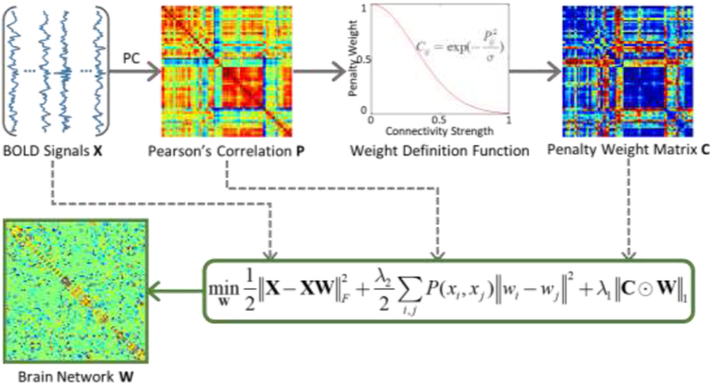
Overview of the proposed WGraphSR framework for brain functional network construction. Given the whole brain BOLD signals X, the Pearson’s correlation (PC) matrix P is computed as the similarity measure corresponding to N ROIs for the graph Laplacian regularizer. The penalty weight matrix C is defined based on the connectivity strength for the weighted ℓ₁-norm. The brain network W is constructed via the proposed optimization framework.

2.1. Graph Laplacian regularization constraint

According to a certain atlas, the whole brain can be parceled into N ROIs, each of which contains an averaged fMRI time course (BOLD signal). We suppose that the time course associated with the i^th ROI is a column vector x_i = [x_1i;x_2i;⋯;x_Mi] ∈ ℝ^M. Then, the whole brain BOLD signals of a subject with N ROIs can be represented by a data matrix X = [x₁, x₂,⋯,x_N] ∈ ℝ^M×N. As a result, the key point for modeling the BFN is to estimate the adjacent matrix W ∈ ℝ^N×N whose entry W_ij represents the relationship or “connectivity” between x_i and x_j.

Based on the manifold assumption, the data tend to reside on a submanifold embedded in the ambient space, and the projected data need to preserve the locality characteristics of the original data in ambient space. The SR modeling can be treated as a “projection” way for the original observed data, and the resultant sparse coefficients as the projected data. With the definition of column vector w_i = [W_1i,W_2i,⋯W_Ni]^T as all connectivity with the i^th ROI, we propose a graph Laplacian regularized constraint as shown in Figure 2 to preserve the local geometry of the manifold structure in the constructed BFN:

$$\frac{1}{2}\sum _{i=1}^N\sum _{j=1}^{N}P(x_i,x_j){\Vert w_i-w_j\Vert }^2,$$ (1)

where P(x_i, x_j) is a non-negative similarity measure between time series x_i and x_j. It is defined as the absolute PC, $P(x_i,x_j)\doteq P_{\mathit{ij}}=\mid x_i^T{x}_j\mid$, where x_i has been centralized and normalized by $x_i\leftarrow \frac{x_i-{\stackrel{‒}{x}}_i}{\sqrt{(x_i-{\stackrel{‒}{x}}_i{)}^T(x_i-{\stackrel{‒}{x}}_i)}}$.

Figure 2.

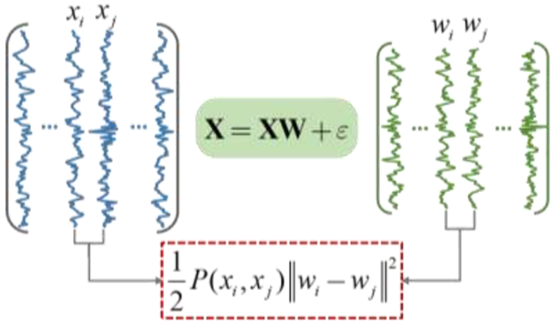
Graph regularized constraint. We suppose that the constructed brain network (with w_i and w_j as the i^th and j^th columns of the adjacent matrix) can preserve the local geometrical structure (measured by the correlation between x_i and x_j) in the original data space.

By minimizing Eq. (1), we can constrain the constructed BFN to keep the local similarity of data in the original space. In other words, a higher correlation P(x_i, x_j) between x_i and x_j will lead to a closer distance between the column vectors w_i and w_j in BFN. Thus, the objective optimization and manifold assumption achieve a congruence.

2.2. Weighted graph regularized sparse model for BFN construction

Based on our previous study [56], the connectivity-strength weighted sparse model (WSR) can combine sparsity and pairwise similarity, which are depicted by ℓ₁-norm and PC, respectively, to model a BFN. It can be formulated as follows:

$$\underset{\{W_{1i},W_{2i},\dots ,W_{Ni}\}}{\min }\frac{1}{2}{\Vert x_i-{\sum }_{j\ne i}{x}_j{W}_{\mathit{ji}}\Vert }_2^2+\lambda {\sum }_{j\ne i}C(x_j,x_i)\mid W_{\mathit{ji}}\mid ,\forall i=1,2,\dots ,N,$$ (2)

where C(x_j, x_i) can be defined as any inverse proportion function of the correlation between x_i and x_j. Thus, a higher correlation will result in a lower penalty, and in turn a weaker constraint on the connectivity |W_ji|. Otherwise, a larger penalty C(x_j, x_i) will “push” |W_ji| to approach zero. However, the WSR model treats the brain regions separately, which may result in an unstable construction. Therefore, we propose a weighted graph regularized SR model that combines the WSR with the newly developed graph Laplacian regularizer in a unified framework to preserve the local manifold structure and similarity prior during the joint BFN construction. The proposed BFN construction model is as follows:

$$\begin{gathered} \underset{\mathrm{W}}{\min }\sum _{i=1}^N\left(\frac{1}{2}{\Vert x_i-\sum _{j\ne i}{x}_j{W}_{\mathit{ji}}\Vert }_2^2+{\lambda }_1\sum _{j\ne i}C(x_j,x_i)\mid W_{\mathit{ji}}\mid \right)+{\lambda }_2\frac{1}{2}\sum _{i=1}^N\sum _{j=1}^{N}P(x_i,x_j){\Vert w_i-w_j\Vert }^2 \\ s.t.W_{\mathit{ii}}=0,\forall i=1,2,\dots ,N \end{gathered}$$ (3)

where C(x_j, x_i) is defined as the exponential function $C_{\mathit{ji}}\doteq C(x_j,x_i)=e^{-\frac{P_{\mathit{ji}}^2}{\sigma }}$, which is selected due to its smoothness and controllable value ranging from 0 to 1. λ₁ and λ₂ are the two trade-off parameters for controlling the balance between the (first) weighted ℓ₁-norm regularization and the (second) graph regularization in the objective function. In order to avoid a trivial solution of W = I, we constrain W_ii = 0. For easier understanding, we define c_i = [C_1i, C_2i,⋯,C_Ni]^T ∈ ℝ^N×1 as a penalty column vector and X⁽ⁱ⁾ = [x₁,x₂,…, x_i−1, 0, x_i+1, …, x_N] ∈ ℝ^M×N as the dictionary for the i^th ROI’s construction, which is equivalent to removing signals of the i^th ROI from the dictionary. Then, Eq. (3) can be rewritten as:

$$\begin{gathered} \underset{\mathrm{W}}{\min }\sum _{i=1}^N\left(\frac{1}{2}{\Vert x_i-{\mathbf{X}}^{(i)}{w}_i\Vert }_2^2+{\lambda }_1{\Vert c_i\odot w_i\Vert }_1\right)+{\lambda }_2\frac{1}{2}\sum _{i=1}^N\sum _{j=1}^N{P}_{\mathit{ij}}{\Vert w_i-w_j\Vert }^2 \\ s.t.W_{\mathit{ii}}=0,\forall i=1,2,\dots ,N. \end{gathered}$$ (4)

In this way, we can integrate constraints on functional connectivity strength, graph regularization, as well as sparsity into a unified framework for a more reasonable BFN.

It is noteworthy that there is a controversial point in the distance measure ‖w_i − w_j‖². To avoid a trivial solution, we need to constrain W_ii and W_jj to be zero in case of self-representation. However, the connectivity W_ij and W_ji are probably non-zero during optimization, especially with a higher correlation between x_i and x_j. As the distance ${\Vert w_i-w_j\Vert }^2$ contains two operations, (W_ii − W_ij)² and (W_ji − W_jj)², which will become (0 − W_ij)² and (W_ji − 0)², it could theoretically result in a high distance even when w_i and w_j are close in the new space. In fact, due to such a distance measure, the optimization algorithm will fail to converge in the experiment. Therefore, we propose to remove both (W_ii − W_ij)² and (W_ji − W_jj)², and define the measurement as ${\Vert w_i-w_j\Vert }^2-{(W_{\mathit{ii}}-W_{\mathit{ij}})}^2-{(W_{\mathit{ji}}-W_{jj})}^2$ to prevent interference of the reasonable BFN construction. The fine-tuned formation is shown as follows:

$$\begin{gathered} \underset{\mathrm{W}}{\min }\sum _{i=1}^N\left(\frac{1}{2}{\Vert x_i-{\mathbf{X}}^{(i)}{w}_i\Vert }_2^2+{\lambda }_1{\Vert c_i\odot w_i\Vert }_1\right) \\ +{\lambda }_2\frac{1}{2}\sum _{i=1}^N\sum _{j=1}^N{P}_{\mathit{ij}}\left[{\Vert w_i-w_j\Vert }^2-{(W_{\mathit{ii}}-W_{\mathit{ij}})}^2-{(W_{\mathit{ji}}-W_{\mathit{jj}})}^2\right] \end{gathered}$$ (5)

With a simplification of the last term, we have the following objective function:

$$\begin{gathered} \underset{\mathrm{W}}{\min }\sum _{i=1}^N\left(\frac{1}{2}{\Vert x_i-{\mathbf{X}}^{(i)}{w}_i\Vert }_2^2+{\lambda }_1{\Vert c_i\odot w_i\Vert }_1\right)+{\lambda }_2\frac{1}{2}\sum _{i=1}^N\sum _{j=1}^N{P}_{\mathit{ij}}{\Vert w_i-w_j\Vert }^2-{\lambda }_2\sum _{i=1}^N\sum _{j=1}^N{P}_{\mathit{ij}}{(W_{\mathit{ii}}-W_{\mathit{ij}})}^2 \\ s.t.W_{\mathit{ii}}=0,\forall i=1,2,\dots ,N \end{gathered}$$ (6)

This is the final WGraphSR model proposed in this paper. Compared with Eq. (4), there is one more term $-{\lambda }_2{\sum }_{i=1}^N{\sum }_{j=1}^N{P}_{\mathit{ij}}(W_{\mathit{ii}}-W_{\mathit{ij}}{)}^2$ introduced for excluding the interference of ${W_{\mathit{ii}}}_{i=1}^N$ on the distance measure. Next, through introducing Laplacian matrix, we sort the objective before optimization. Specifically, we define the degree of x_i as $d_i={\sum }_{i=1}^N{P}_{\mathit{ij}}$ and let D = diag(d₁, ⋯, d_N). Then we have

$$\begin{gathered} \frac{1}{2}\sum _{i=1}^N\sum _{j=1}^N{P}_{\mathit{ij}}{\Vert w_i-w_j\Vert }^2 \\ =\mathrm{Tr}({\mathbf{WLW}}^T)=\mathrm{Tr}(\sum _{i=1}^N\sum _{j=1}^N{L}_{\mathit{ij}}{w}_i{w}_j^T)=\sum _{i=1}^N\sum _{j=1}^N{L}_{\mathit{ij}}{w}_j^T{w}_i=\sum _{i=1}^N\sum _{j=1}^N{L}_{\mathit{ij}}{w}_i^T{w}_j \end{gathered}$$ (7)

where L = D-P is the Laplacian matrix and Tr(⋅)is the trace of a matrix. The objective function is rewritten as:

$$\begin{gathered} \underset{\mathrm{W}}{\min }\sum _{i=1}^N\left(\frac{1}{2}{\Vert x_i-{\mathbf{X}}^{(i)}{w}_i\Vert }_2^2+{\lambda }_1{\Vert c_i\odot w_i\Vert }_1\right)+{\lambda }_2\sum _{i=1}^N\sum _{j=1}^N{L}_{\mathit{ij}}{w}_i^T{w}_j-{\lambda }_2\sum _{i=1}^N\sum _{j=1}^N{P}_{\mathit{ij}}{(W_{\mathit{ii}}-W_{\mathit{ij}})}^2 \\ s.t.W_{\mathit{ii}}=0,\forall i=1,2,\dots ,N \end{gathered}$$ (8)

Next, by expanding the last quadratic term and then using the definition of ${\sum }_{j=1}^N{P}_{\mathit{ij}}=d_i$, we have the following objective function:

$$\begin{gathered} \underset{\mathrm{W}}{\min }\sum _{i=1}^N\left(\frac{1}{2}{\Vert x_i-{\mathbf{X}}^{(i)}{w}_i\Vert }_2^2+{\lambda }_1{\Vert c_i\odot w_i\Vert }_1\right)+{\lambda }_2\sum _{i=1}^N\sum _{j=1}^N{L}_{\mathit{ij}}{w}_i^T{w}_j \\ -{\lambda }_2\left[\sum _{i=1}^N{W}_{\mathit{ii}}^2{d}_i-2\sum _{i=1}^N\sum _{j=1}^N{P}_{\mathit{ij}}{W}_{\mathit{ii}}{W}_{\mathit{ij}}+\sum _{i=1}^N\sum _{j=1}^N{P}_{\mathit{ij}}{W}_{\mathit{ij}}^2\right] \\ s.t.W_{\mathit{ii}}=0,\forall i=1,2,\dots ,N \end{gathered}$$ (9)

2.3. Algorithm

We propose to solve the optimization problem by vectorizing the connectivity matrix W = w₁, w₂, …, w_N ∈ ℝ^N×N as $\tilde{W}={[w_1^T,w_2^T,\dots ,w_N^T]}^T\in {ℝ}^{\mathit{NN}\times 1}$. By defining the matrix dictionary $\mathbf{A}={\left[\begin{array}{cccc}\hfill {\mathbf{X}}^{(1)}\hfill & \hfill 0\hfill & \hfill \cdots \hfill & \hfill 0\hfill \\ \hfill 0\hfill & \hfill {\mathbf{X}}^{(2)}\hfill & \hfill 0\hfill & \hfill ⋮\hfill \\ \hfill ⋮\hfill & \hfill 0\hfill & \hfill \ddots \hfill & \hfill 0\hfill \\ \hfill 0\hfill & \hfill \cdots \hfill & \hfill 0\hfill & \hfill {\mathbf{X}}^{(\mathbf{N})}\hfill \end{array}\right]}_{\mathit{MN}\times \mathit{NN}}$, the vectorized observed data $\tilde{X}={[x_1^T,x_2^T,\dots ,x_N^T]}^T\in {ℝ}^{\mathit{MN}\times 1}$ and the new weight matrix $\tilde{\mathbf{C}}=\mathit{diag}{[c_1^T,c_2^T,\dots ,c_N^T]}^T\in {ℝ}^{\mathit{NN}\times \mathit{NN}}$ respectively. As a result, the fitting term and the first weighted sparse regularization can be rewritten as follows:

$$\sum _{i=1}^N\left(\frac{1}{2}{\Vert x_i-{\mathbf{X}}^{(i)}{w}_i\Vert }_2^2+{\lambda }_1{\Vert c_i\odot w_i\Vert }_1\right)=\frac{1}{2}{\Vert \tilde{X}-\mathbf{A}\tilde{W}\Vert }_2^2+{\lambda }_1{\Vert \tilde{\mathbf{C}}\tilde{W}\Vert }_1$$ (10)

For the remaining terms, we denote ${\tilde{\mathbf{L}}}_{\mathbf{ij}}={\left[\begin{array}{cccc}\hfill L_{\mathit{ij}}\hfill & \hfill 0\hfill & \hfill \cdots \hfill & \hfill 0\hfill \\ \hfill 0\hfill & \hfill L_{\mathit{ij}}\hfill & \hfill \hfill & \hfill ⋮\hfill \\ \hfill ⋮\hfill & \hfill \hfill & \hfill \ddots \hfill & \hfill 0\hfill \\ \hfill 0\hfill & \hfill \cdots \hfill & \hfill 0\hfill & \hfill L_{\mathit{ij}}\hfill \end{array}\right]}_{N\times N}$, and then have ${\sum }_{i=1}^N{\sum }_{j=1}^N{L}_{\mathit{ij}}{w}_j^T{w}_i={\sum }_{i=1}^N{\sum }_{j=1}^N{L}_{\mathit{ji}}{w}_j^T{w}_i={\sum }_{i=1}^N{\sum }_{j=1}^N{L}_{\mathit{ji}}{w}_j^T\mathbf{I}{w}_i={\sum }_{i=1}^N{\sum }_{j=1}^N{w}_j^T{\tilde{\mathbf{L}}}_{\mathbf{ji}}{w}_i={\tilde{W}}^T{\tilde{\mathbf{L}}}^{(1)}\tilde{W}$, where ${\tilde{\mathbf{L}}}^{(1)}={\left[\begin{array}{cccc}\hfill {\tilde{\mathbf{L}}}_{11}\hfill & \hfill {\tilde{\mathbf{L}}}_{12}\hfill & \hfill \cdots \hfill & \hfill {\tilde{\mathbf{L}}}_{1N}\hfill \\ \hfill {\tilde{\mathbf{L}}}_{21}\hfill & \hfill {\tilde{\mathbf{L}}}_{22}\hfill & \hfill \hfill & \hfill {\tilde{\mathbf{L}}}_{2N}\hfill \\ \hfill ⋮\hfill & \hfill \hfill & \hfill \ddots \hfill & \hfill ⋮\hfill \\ \hfill {\tilde{\mathbf{L}}}_{N1}\hfill & \hfill {\tilde{\mathbf{L}}}_{N2}\hfill & \hfill \cdots \hfill & \hfill {\tilde{\mathbf{L}}}_{\mathbf{NN}}\hfill \end{array}\right]}_{\mathit{NN}\times \mathit{NN}}$.

Denoting ${\tilde{\mathbf{L}}}^{(2)}=\mathit{diag}(D(:))$, we have ${\sum }_{i=1}^N{W}_{\mathit{ii}}^2{d}_i={\tilde{W}}^T{\tilde{\mathbf{L}}}^{(2)}\tilde{W}$. Next, denote ${\tilde{\mathbf{L}}}^{\left(3\right)}={\left[\begin{array}{ccccccccc}\hfill I_{11}\hfill & \hfill 0\hfill & \hfill \cdots \hfill & \hfill 0\hfill & \hfill \hfill & \hfill I_{11}\hfill & \hfill \hfill & \hfill \hfill & \hfill \hfill \\ \hfill 0\hfill & \hfill ⋮\hfill & \hfill \hfill & \hfill \hfill & \hfill \hfill & \hfill \hfill & \hfill \hfill & \hfill \hfill & \hfill \hfill \\ \hfill \hfill & \hfill I_{22}\hfill & \hfill \hfill & \hfill ⋮\hfill & \hfill \cdots \hfill & \hfill \hfill & \hfill I_{22}\hfill & \hfill \hfill & \hfill \hfill \\ \hfill ⋮\hfill & \hfill 0\hfill & \hfill \ddots \hfill & \hfill \hfill & \hfill \hfill & \hfill \hfill & \hfill \hfill & \hfill \ddots \hfill & \hfill \hfill \\ \hfill \hfill & \hfill ⋮\hfill & \hfill \hfill & \hfill 0\hfill & \hfill \hfill & \hfill \hfill & \hfill \hfill & \hfill \hfill & \hfill \hfill \\ \hfill 0\hfill & \hfill \cdots \hfill & \hfill 0\hfill & \hfill I_{\mathit{NN}}\hfill & \hfill \hfill & \hfill \hfill & \hfill \hfill & \hfill \hfill & \hfill I_{\mathit{NN}}\hfill \end{array}\right]}_{\mathit{NN}\times \mathit{NN}}{\left[\begin{array}{cccccc}\hfill P_{11}\hfill & \hfill 0\hfill & \hfill \hfill & \hfill \cdots \hfill & \hfill \hfill & \hfill 0\hfill \\ \hfill 0\hfill & \hfill P_{21}\hfill & \hfill \hfill & \hfill \hfill & \hfill \hfill & \hfill 0\hfill \\ \hfill \hfill & \hfill \hfill & \hfill P_{31}\hfill & \hfill \hfill & \hfill \hfill & \hfill \hfill \\ \hfill ⋮\hfill & \hfill ⋮\hfill & \hfill ⋮\hfill & \hfill \ddots \hfill & \hfill \hfill & \hfill ⋮\hfill \\ \hfill \hfill & \hfill \hfill & \hfill \hfill & \hfill \hfill & \hfill P_{N-1N}\hfill & \hfill 0\hfill \\ \hfill 0\hfill & \hfill 0\hfill & \hfill \hfill & \hfill \cdots \hfill & \hfill 0\hfill & \hfill P_{\mathit{NN}}\hfill \end{array}\right]}_{\mathit{NN}\times \mathit{NN}}$, and we get ${\sum }_{i=1}^N{\sum }_{j=1}^N{P}_{\mathit{ij}}{W}_{\mathit{ii}}{W}_{\mathit{ij}}={\tilde{W}}^T{\tilde{\mathbf{L}}}^{(3)}\tilde{W}$. Denote ${\tilde{\mathbf{L}}}^{(4)}=\mathit{diag}(P(:))$ to get ${\sum }_{i=1}^N{\sum }_{j=1}^N{P}_{\mathit{ij}}{W}_{\mathit{ij}}^2={\tilde{W}}^T{\tilde{\mathbf{L}}}^{(4)}\tilde{W}$ .

It is worthwhile to note that the rewriting of the last constraint aims at unifying the formations to ${\tilde{W}}^T{\tilde{\mathbf{L}}}^{(\ast )}\tilde{W}$. Finally, we denote $\tilde{\mathbf{L}}={\tilde{\mathbf{L}}}^{(1)}-{\tilde{\mathbf{L}}}^{(2)}+2{\tilde{\mathbf{L}}}^{(3)}-{\tilde{\mathbf{L}}}^{(4)}$, and then Eq. (9) is equivalent to the following:

$$\underset{\tilde{W}}{\min }\frac{1}{2}{\Vert \tilde{X}-\mathbf{A}\tilde{W}\Vert }_2^2+{\lambda }_1{\Vert \tilde{\mathbf{C}}\tilde{W}\Vert }_1+{\lambda }_2{\tilde{W}}^T\tilde{\mathbf{L}}\tilde{W}.$$ (11)

For solving this optimization problem, we introduce a variable $\tilde{V}$, and then get:

$$\underset{\tilde{W},\tilde{V},\mu }{\min }\frac{1}{2}{\Vert \tilde{X}-\mathbf{A}\tilde{W}\Vert }_2^2+{\lambda }_1{\Vert \tilde{\mathbf{C}}\tilde{V}\Vert }_1+{\lambda }_2{\tilde{W}}^T\tilde{\mathbf{L}}\tilde{W},s.t.\tilde{W}=\tilde{V}.$$

Based on the alternating direction method of multipliers (ADMM), we have:

$$\underset{\tilde{W},\tilde{V},\mu }{\min }f(\tilde{W},\tilde{V},\mu )=\frac{1}{2}{\Vert \tilde{X}-\mathbf{A}\tilde{W}\Vert }_2^2+{\lambda }_1{\Vert \tilde{\mathbf{C}}\tilde{V}\Vert }_1+{\lambda }_2{\tilde{W}}^T\tilde{\mathbf{L}}\tilde{W}+\langle \mu ,\tilde{W}-\tilde{V}\rangle +\frac{\rho }{2}{\Vert \tilde{W}-\tilde{V}\Vert }_2^2$$

In particular, we first initialize ${\tilde{V}}^0=\overrightarrow{0}$, ${\mu }^0=\overrightarrow{0}$, and then solve one of the three variables $\tilde{W}$, $\tilde{V}$ and μ alternately, until the iterative stop requirement is achieved. 1) Fix variables $\tilde{V}$ and μ, and solve $\tilde{W}:{\tilde{W}}^{k+1}≔\underset{\tilde{W}}{\arg \min }f(\tilde{W},{\tilde{V}}^k,{\mu }^k)$ The objective function to be optimized is

$$\frac{1}{2}{\Vert \tilde{X}-\mathbf{A}\tilde{W}\Vert }_2^2+{\lambda }_2{\tilde{W}}^T\tilde{\mathbf{L}}\tilde{W}+\frac{\rho }{2}{\Vert \tilde{W}-{\tilde{V}}^k+\frac{{\mu }^k}{\rho }\Vert }_2^2.$$

Derivate it by $\tilde{W}$ to get

$$({\mathbf{A}}^T\mathbf{A}+2{\lambda }_2\tilde{\mathbf{L}}+\rho \mathbf{I})\tilde{W}={\mathbf{A}}^T\tilde{X}+\rho {\tilde{V}}^k-{\mu }^k.$$

To avoid the inverse operation, we adopt the conjugate gradient method to solve $\tilde{W}$. 2) Fix variables $\tilde{W}$ and μ, and solve $\tilde{V}:{\tilde{V}}^{k+1}:=\underset{\tilde{V}}{\arg \min }f({\tilde{W}}^{k+1},\tilde{V},{\mu }^k)$ The objective function to be optimized is

$${\lambda }_1{\Vert \tilde{\mathbf{C}}\tilde{V}\Vert }_1+\frac{\rho }{2}{\Vert {\tilde{W}}^{k+1}-\tilde{V}+\frac{{\mu }^k}{\rho }\Vert }_2^2\to \frac{1}{2}{\Vert \tilde{V}-({\tilde{W}}^{k+1}+\frac{{\mu }^k}{\rho })\Vert }_2^2+\frac{{\lambda }_1}{\rho }{\Vert \tilde{\mathbf{C}}\tilde{V}\Vert }_1.$$

Using the soft threshold method, we get

$${\tilde{V}}^{k+1}=\text{shrinkage}({\tilde{W}}^{k+1}+\frac{{\mu }^k}{\rho },\frac{{\lambda }_1}{\rho }\text{diag}(\tilde{\mathbf{C}})).$$

3) Fix variables $\tilde{W}$ and $\tilde{V}$, and solve μ:

$${\mu }^{k+1}≔{\mu }^k+\rho ({\tilde{W}}^{k+1}-{\tilde{V}}^{k+1})$$

The detailed algorithm procedure of WGraphSR is described in Algorithm 1. Since the structured sparse model will achieve an asymmetrical result, we symmetrize the BFN by a simple strategy of W ←(W+W^T)/2. Next, with the constructed BFNs we will identify subjects with MCI from normal controls.

Table I.

Network construction models with different data-fitting and regularization terms.

Construction model	Data-fitting term	Regularization term
PC	${\Vert W-X^{T}X\Vert }_F^2$	—
SR	$\frac{1}{2}{\Vert X-\mathrm{XW}\Vert }_F^2$	$\lambda {\Vert \mathbf{W}\Vert }_1$
WSR	$\frac{1}{2}{\Vert X-\mathrm{XW}\Vert }_F^2$	$\lambda {\Vert \mathbf{C}\odot \mathbf{W}\Vert }_1$
WSGR	$\frac{1}{2}{\Vert X-\mathrm{XW}\Vert }_F^2$	${\lambda }_1{\Vert \mathbf{C}\odot \mathbf{W}\Vert }_1+{\lambda }_2{\sum }_{k=1}^K{d}_k{\Vert W_{G_k}\Vert }_q$
WGraphSR	$\frac{1}{2}{\Vert X-\mathrm{XW}\Vert }_F^2$	${\lambda }_1{\Vert \mathbf{C}\odot \mathbf{W}\Vert }_1+{\lambda }_2\mathrm{Tr}\left({\mathbf{WLW}}^T\right)$

Algorithm 1.

Learning Weighted Graph Regularized Sparse Representation Input

Input: Mean BOLD time series X = [x1,x2,…,xi,…,xN] ∈ ℝM×N, λ1 >0, λ2 >0

Initialize: $\tilde{X}=\mathrm{vec}\left(X\right)$, X(i) = [x1,x2,…,xi−1, 0, xi+1, …, xN],

A = diag(X(1),X(2),…,X(N)), ρ=100, abstol=10−4, reltol=10−2,

max Iter=1000, ${\tilde{V}}^0=\overrightarrow{0}$, ${\mu }^0=\overrightarrow{0}$

For k = 0: max Iter−1

1) Update variable $\tilde{W}$ with conjugate gradient method

$\frac{1}{2}{\Vert \tilde{X}-\mathbf{A}\tilde{W}\Vert }_2^2+{\lambda }_2{\tilde{W}}^T\tilde{\mathbf{L}}\tilde{W}+\frac{\rho }{2}{\Vert \tilde{W}-{\tilde{V}}^k+\frac{{\mu }^k}{\rho }\Vert }_2^2$

$({\mathbf{A}}^T\mathbf{A}+2{\lambda }_2\tilde{\mathbf{L}}+\rho \mathbf{I})\tilde{W}={\mathbf{A}}^T\tilde{X}+\rho {\tilde{V}}^k-{\mu }^k$

2) Update variable $\tilde{V}$

${\tilde{V}}^{k+1}=\text{shrinkage}({\tilde{W}}^{k+1}+\frac{{\mu }^k}{\rho },\frac{{\lambda }_1}{\rho }\mathit{diag}(\tilde{\mathbf{C}}\left)\right)$

3) Update Lagrange multiplier μ

${\mu }^{k+1}≔{\mu }^k+\rho ({\tilde{W}}^{k+1}-{\tilde{V}}^{k+1})$

4) Check the convergence

$\mathbf{IF}{\Vert {\tilde{W}}^{k+1}-{\tilde{V}}^{k+1}\Vert }_2<{N^2}^{\ast }\mathrm{abs}\mathit{tol}+\mathrm{rel}{\mathit{tol}}^{\ast }\max ({\Vert {\tilde{W}}^{k+1}\Vert }_2,{\Vert -{\tilde{V}}^{k+1}\Vert }_2)$ &&

${\Vert -\rho ({\tilde{V}}^{k+1}-{\tilde{V}}^k\Vert }_2<{N^2}^{\ast }\mathrm{abs}\mathit{tol}+\mathrm{rel}{\mathit{tol}}^{\ast }{\Vert {\mu }^{k+1}\Vert }_2\text{then}$

break;

end IF

end For

Output: $(\tilde{W},\tilde{V})$ Rearrange $\tilde{W}$ as its matrix form W

3. Experiments

The rs-fMRI data are downloaded from Alzheimer’s Disease Neuroimaging Initiative (ADNI) [65]. Specifically, there are ninety-nine subjects in total, with forty-nine normal controls and fifty MCI patients, selected from the ADNI phase-2 dataset. Participants from both groups are age- and gender-matched, and they were all scanned with the same protocol using 3.0T Philips Achieva scanners. The details of imaging parameters are listed as follows: repetition time (TR) = 3 s, echo time (TE) = 30 ms, flip angle = 80°, imaging matrix = 64×64, 48 slices, slice thickness = 3.3 mm, and 140 volumes (time points) for each subject. The image pre-processing for all rs-fMRI data is performed with the SPM8 toolbox (http://www.fil.ion.ucl.ac.uk/spm/) according to a standard pipeline [24], including volume removal, slice timing correction, head motion correction, normalization and spatial smoothing. Specifically, the first three volumes of each subject are discarded for steady-state tissue magnetization equilibrium. Then head motion correction is achieved by a rigid-body registration. The fMRI images are normalized to the Montreal Neurological Institute (MNI) space and spatially smoothed with a Gaussian kernel with full-width-at-half-maximum (FWHM) of 6×6×6 mm³. To reduce the negative effect on network study caused by head motion, we exclude partial fMRI data from further analysis [66] if it contains: 1) overall head motion larger than 2 mm or 2 degrees; 2) more than 2.5 min (50 frames) data of frame-wise displacement > 0.5. Finally, the whole brain in rs-fMRI space is parceled into a number of ROIs by warping the Automated Anatomical Labeling (AAL) template [31] to the original rs-fMRI space, and the averaged BOLD time series is extracted from each ROI. Head motion parameters (i.e., Friston-24 model) and the mean time series of white matter and cerebrospinal fluid are regressed out from the band-pass filtered (0.01–0.08 Hz) rs-fMRI data.

3.1. Brain functional network construction

For a comprehensive comparison, we construct BFN using basic methods (i.e., PC and SR), two modified methods including WSR and weighted sparse group representation (WSGR), and our proposed method WGraphSR. Their matrix-regularized objective functions are provided in Table I.

In Figure 3, we visualize the BFNs from a randomly-selected subject constructed using the five different methods. The traditional PC-based network is shown in Figure 3(a), where the modular characteristic can be confirmed. All the BFNs constructed from the SR models are sparse. In terms of the connectivity-strength weight, we can conclude that the sparse constraint with penalty weights (Figure 3(c)-3(e)) could preserve more modular characteristics in modeling the BFN than that without weights (Figure 3(b)). Regarding the graph Laplacian regularizer for manifold structure preservation, we calculate the correlation matrix of network constructed by our proposed WGraphSR in Figure 3(f). Comparing with Figure 3(a) and (f), we can observe that the correlation between original BOLD signals x_i. and x_j are highly similar to the correlation between constructed regional connectivity series w_i and w_j, which demonstrates that our proposed model can preserve the underlying local geometry of the manifold structure of rs-fMRI data.

Figure 3.

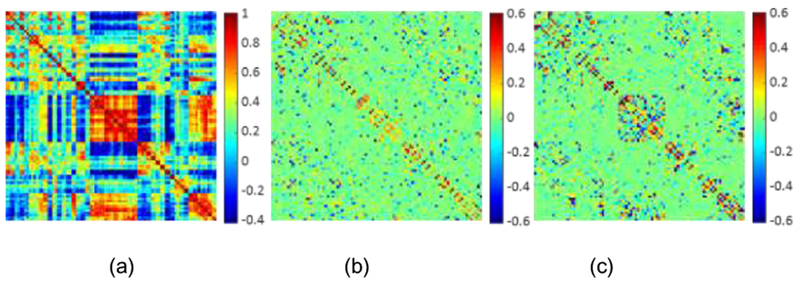
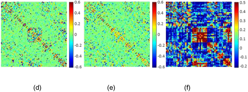
Illustration of the BFNs constructed by different models, and the manifold structure preservation. (a) Network based on PC; (b) network based on SR; (c) network based on WSR; (d) network based on WSGR; (e) network based on WGraphSR; (f) the correlation measurement of brain network from (e).

3.2. Feature selection

The constructed BFN delineates all the connectivity information between ROIs. However, due to the fact that human brains share several common connectome patterns across subjects, the separately constructed BFNs contain redundant information for identifying the biomarkers of brain diseases. Additionally, the high-dimensional network data and limited training samples will pose a challenge to the disease prediction. Therefore, in this work, we propose a sparse feature selection strategy to take the interaction of features into account and select discriminative features jointly. Specifically, a linear regression with a sparse constraint, i.e., LASSO, composes the selection model as shown in Figure 4.

Figure 4.

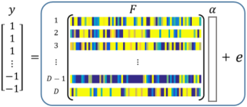
Feature selection by LASSO. Each row of the matrix F ∈ ℝ^D×E is formatted by all the E connectivity features of the constructed BFN. There are D sets of training data in this process.

Suppose we have D training samples with true labels y ∈ ℝ^D×1, where MCI patients are labeled with +1, and healthy controls are labeled with −1. We regress the combination of connectivity features to the corresponding label as follows:

$$\underset{\alpha }{\min }\frac{1}{2}{\Vert y-\mathbf{F}\alpha \Vert }_2^2+{\lambda }_{\mathit{FS}}{\Vert \alpha \Vert }_1,$$ (12)

and choose the features with non-zero coefficients as the selected feature indices (SFI).

$$\mathrm{SFI}=\{\mid {\alpha }_i\ne 0,i=1,2,\cdots E\}$$ (13)

Based on LASSO, all the selected features are non-independent and belong to the jointly selected most discriminative feature subset. Meanwhile, with the introduction of sparsity, the magnitude of the resulting subset is much smaller than the original feature dimensionality.

3.3. MCI classification results

The functional connectivity within the constructed brain network will be treated as features for MCI classification. Through the sparse feature selection, the new training data will be achieved by reducing the network connectivity according to SFI. We regard the selected connectivity as the final features to train a classifier for MCI identification. To validate the effectiveness of the proposed network construction model, the leave-one-out cross validation (LOOCV) strategy is adopted for making full use of the limited data. Specifically, three parameters are involved in the training stage, including λ₁ and λ₂ in the network construction model, and λ_FS in the feature selection step. To set the values of these regularization parameters, we employ a nested LOOCV strategy on the training set to grid-search the optimal parameter values. For the regularized parameters λ₁ and λ₂, the candidate values are [2 ⁻⁵, 2⁻⁴, ⋯ , 2¹, 2²]. For the sparse regularized parameter, we have λ_FS = ratio* λ_max, where λ_max is automatically computed as the maximal value of λ_FS, above which Eq. (12) will obtain a zero solution [67]. The candidate values for the parameter ratio are from [0.1,0.2, ⋯ ,0.6]. Given S subjects involved in our study, S −1 subjects are used for training while the left-out one is used for testing. This procedure is repeated S times for evaluating the classification performance. During each repeat, the nested LOOCV is carried out on the S −1 training subjects to select the optimal parameters that contribute to the best performance on the training sets. Then, by applying the optimal parameters on the S −1 different training subsets, we train S −1 linear support vector machines (SVMs) to classify the test subject, and the final classification result is determined via majority voting. Finally, after repeating the above process S times, an overall cross-validation classification accuracy is calculated.

Different statistical evaluation measurements are listed below to evaluate classification performance, where TP, TN, FP, and FN denote true positive, true negative, false positive, and false negative, respectively, and precision=TP/(TP+FP) and recall= TP/(TP+FN). In this paper, MCI samples are treated as the positive class. The statistical experimental results on real rs-fMRI data are shown in Table II. The receiver operating characteristic (ROC) curves showing the different classification performances of these construction methods are given in Figure 5, while the statistical index area under ROC curve (AUC) is listed in Table II.

Table II.

Comparison of classification results by different methods.

Construction models	ACC	SEN	SPE	AUC	F-score
PC	57.58	62.00	53.06	60.01	59.62
SR	65.66	62.00	69.39	66.66	64.58
WSR	79.80	80.00	79.59	85.44	80.00
WSGR	84.85	92.00	77.55	91.59	85.98
WGraphSR	88.89	88.00	89.80	92.32	88.89

Figure 5.

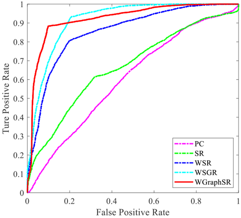
ROC curves corresponding to five network construction models.

$$\text{Accuracy}(\mathrm{ACC})=\frac{\mathit{TP}+\mathit{TN}}{\mathit{TP}+\mathit{FP}+\mathit{TN}+\mathit{FN}}\text{Sensitivity}(\mathrm{SEN})=\frac{\mathit{TP}}{\mathit{TP}+\mathit{FN}}$$

$$\text{Specificity}(\mathrm{SPE})=\frac{\mathit{TN}}{\mathit{TN}+\mathit{FP}}\text{F-Score}=2\times \frac{\text{precision}\times \text{recall}}{\text{precision}+\text{recall}}$$

It can be seen that the proposed WGraphSR model for BFN construction achieves the best classification performance with an accuracy of 88.89%, resulting in a 5% and 9% increase in accuracy compared with the previous WSGR model (84.85% accuracy) and the WSR (79.80% accuracy), respectively. This means that our proposed graph Laplacian and the weighted sparse regularizations are able to explore the potential data relationship and further construct a more biologically meaningful BFN, thus identifying more discriminative biomarkers for classifying subjects with MCI from healthy controls. In Table II, it should be noted that the true positive rate and the sensitivity indicator of the WSGR are 4% higher than the proposed method. This indicates that the proposed WGraphSR method recognizes a relatively lower proportion of MCI patients than the WSGR, which needs to be improved in the follow-up work. For the true negative rate/specificity indicator, however, our proposed method is overwhelmingly superior to all other competitive methods, meaning that much less normal healthy controls are misclassified as MCI patients.

4. Discussion

4.1. Most discriminative features

During the sparse feature selection process in each validation step, the selected features for classification might be different for different training datasets. Thus, we record all the selected discriminative features to analyze the biomarkers in MCI identification. With the sparse selection, twenty-two connectivity features were consistently selected in almost all validation sets, as shown in Figure 6. In the circular graph, the red points and red arcs represent, respectively, the brain regions and connectivity features related to the default mode network (DMN), which is commonly regarded as AD-pathology related [68]. The other consistently-selected discriminative features outside of the DMN are shown with grey arcs, which include the connectivity between olfactory cortices, putamen, insula, etc.

Figure 6.

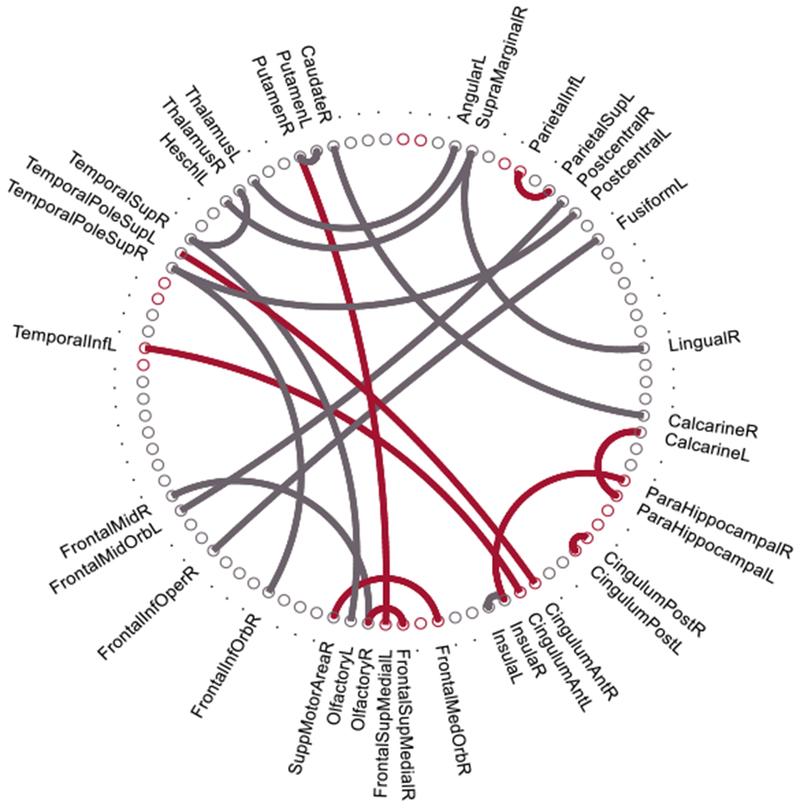
The twenty-two consistently-selected discriminative connectivity features (selected by above 95% of all validations). The red arcs represent the connectivity features related to the default mode network.

The linear SVM classifier trained in each cross-validation is actually a maximum margin hyper-plane, composed of the learned weight coefficients corresponding to all selected features. To further investigate the connectivity pattern that contributes to MCI classification, we analyze the linear classification model to reveal the importance of the selected features by averaging the classification weight coefficients of each selected feature in all folds of cross-validation. The statistical averaged weights of the connectivity features in the linear classifier are shown in Figure 7 with a full brain view, where the nodes represent the ROIs, the node size indicates the degree of the node in the brain network, the edge represents the connectivity feature, and the edge thickness indicates its weight coefficient of the classification plane. The detailed weight coefficients corresponding to all selected features can be found in Supplementary Table I. Within the linear classifier, there are both positive and negative weight coefficients, which are shown in red and blue, respectively.

Figure 7.

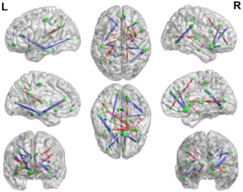
Classification Pattern. The thickness of each edge indicates respective weight used in a linear SVM model for MCI classification. Red/blue edges represent positive/negative weights in the linear model.

For the most discriminative ROIs related to MCI identification, we analyze the connected regions among those consistently selected features displayed in Table III, where the order number and the ROI name are based on the AAL atlas. Twelve discriminative ROIs are shown in Figure 8 with a full brain view. Specifically, the left anterior cingulate, whole posterior cingulate gyrus, left paraHippocampal gyrus, and left inferior temporal are all within the brain DMN, which corroborates exiting studies [69–71] that have pointed out that patients with MCI and AD have the same regional network connectivity anomalies in DMN compared with healthy controls. The right olfactory cortex is highly related to AD pathology, according to previous studies [72]. The subcortical regions of the left putamen, right putamen and hippocampal gyrus are important for MCI identification [73].

Table III.

The information of related ROIs within the consistently selected connectivity features. The order number and name are based on AAL template.

The order number and name of ROI A		The order number and name of ROI B
8	Middle frontal gyrus (right)	22	Olfactory (right)
31	Anterior cingulate gyrus (left)	89	Inferior temporal (left)
35	Posterior cingulate gyrus (left)	36	Posterior cingulate gyrus (right)
39	ParaHippocampal gyrus (left)	43	Calcarine cortex (left)
48	Lingual gyrus (right)	64	Supramarginal gyrus (right)
73	Putamen (left)	74	Putamen (right)

Figure 8.

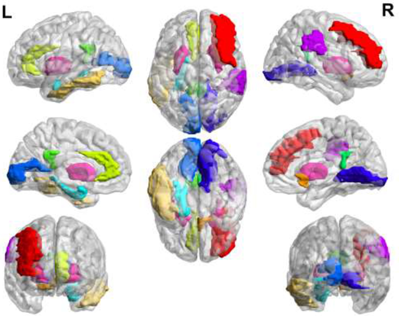
The discriminative regions selected in MCI classification are shown in different colors for better visualization.

4.2. Sensitivity analysis of the regularized parameters

In this paper, there are three regularized parameters, namely λ₁ and λ₂ involved in the BFN construction, as well as λ_FS involved in the feature selection stage. To study the influence of these parameters on the classification performance, we further implement an experiment to identify subjects with MCI from healthy controls under different combination of parametric values. The corresponding classification accuracy of our proposed construction model is calculated using the LOOCV strategy. Due to the facts that 1) it is difficult to show four-dimensional coordinates when considering three variables and 2) the BFN construction model contributes more in the experimental results, we show classification accuracy in Figure 9 with the parameter λ_FS =0.3. It can be observed that the accuracy varies with different values of the regularized parameters, and the best accuracy (93.94%) is achieved with λ₁ = 2⁻⁵ for weighted sparsity and λ₂ = 2⁻² for graph Laplacian regularization term. Overall, it can be seen that the regularized parameter of graph Laplacian has a great influence on experimental results, indicating that our proposed graph regularized constraint plays a more important role in constructing BFNs.

Figure 9.

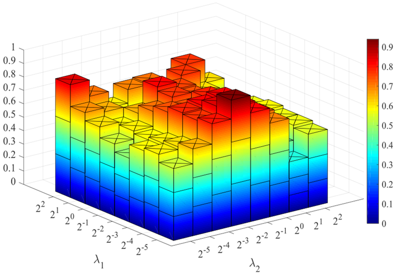
Statistical classification accuracy based on the networks estimated by our proposed method with different values of regularization parameters. For clear visualization, feature selection parameter is set to λ_FS = 0.3. The results are obtained by LOOCV on all data.

4.3. Remarks on WGraphSR and other sparse representative models

In this study, we propose WGraphSR model for BFN construction. Compared with the traditional correlation-based and SR-based methods, our proposed model gets the best of both worlds and takes the relationship between brain network connections into account. WSR, WSGR, and our proposed model all aim to model the similarity preservation problem, although their formulations are quite different. The difference between WSR and WSGR is that the former constrains each connection in the network to be similar to the corresponding correlation independently, while the latter not only constrains the independent connection, but also the group connections to maintain the similarity by the corresponding weighted penalty. Comprehensively speaking, the WSR and WSGR models intend to force the new constructed brain connectivity with the sparsity premise to approximate the traditional correlation between the original regional signals as close as possible. However, none of these models explores the locality involved in the brain connections. The graph-regularized constraint is proposed in this paper to preserve the underlying local geometry of the manifold structure in the data. The network sparsity, weighted penalty based on similarity, and the graph Laplacian regularization based on manifold assumption are combined in a single framework to formulate the WGraphSR construction model. Furthermore, the graph regularization is able to constrain the local manifold structure after reconstruction.

5. Conclusion

The connectivity measurement within the brain network from rs-fMRI data is a fundamental challenge in network-based analysis. In this paper, a novel network construction method based on a graph regularized weighted sparse model is proposed for the study of BFNs. This model could preserve the locality and similarity characteristics among the rs-fMRI data during sparse reconstruction. Moreover, with the connectivity-strength weighted penalty, our proposed WGraphSR model integrates correlation analysis, sparsity constraint, and graph regularized constraint into a unified learning framework that moves toward a more biologically meaningful brain connectome. We further adopt a sparse feature selection strategy to take into account the interaction between features, and comprehensively extract the discriminant feature subset. The effectiveness of our proposed method has been demonstrated by classification experiments in MCI and healthy controls. The experimental results show that our proposed method can identify degenerative disease more effectively than other competitive methods. Through subsequent sensitivity analysis of regularized parameters, our proposed graph regularization constraint based on manifold assumption plays an important role in effective construction of brain network as well as classification of disease.

Highlights.

• Integrate the data similarity and locality to sparse modeling of brain functional network.

• A unified framework integrates intrinsic correlation, local manifold structure, and sparsity.

• Solve the controversial point of graph Laplacian in the self-representation model.

• MCI classification based on fMRI shows our method is more effective (accuracy=8 8.89%).

Author Biographies

Renping Yu received the B.Sc degree in mathematics and Ph.D. degree in control science and engineering from Nanjing University of Science and Technology, Nanjing, China in 2012 and 2017, respectively. From 2015 to 2016, she has visited the department of Radiology and BRIC in University of North Carolina, at Chapel Hill as a joint Ph.D. student for one year. She currently works at the Zhengzhou University, where she became a scientific researcher at the School of Electrical Engineering. Her research interests mainly focus on medical image processing, including brain MRI segmentation and brain network construction.

Lishan Qiao received the B.Sc. degree in mathematics from Liaocheng University (LU) in 2001. He received the M.Sc. degree in applied mathematics from Chengdu University of Technology in 2004, and then worked in LU to this day. In 2010, he received the Ph.D. degree in computer science, at the Department of Computer Science & Engineering, Nanjing University of Aeronautics and Astronautics. Currently, he is an associate professor at School of Mathematics Science, LU, and his research interests mainly focus on pattern recognition, machine learning, and functional brain network analysis. In these fields, he has published more than 20 papers, and one paper won the Biennial Pattern Recognition Journal 2010 Best Paper Award Honorable Mention.

Mingming Chen received the B.Sc. degree in mathematics and applied mathematics from the Changsha University of Science & Technology, Changsha, China in 2010. He received the Ph.D. degree in Biomedical Engineering from the University of Electronic Science and Technology of China in 2017. He currently works at the Zhengzhou University, where he became a scientific researcher at the School of Electrical Engineering. His research interests mainly focus on computational neuroscience, nonlinear dynamic system, EEG processing and brain network analysis.

Seong-Whan Lee received the B.S. degree in computer science and statistics from Seoul National University, Seoul, in 1984, and the M.S. and Ph.D. degrees in computer science from the Korea Advanced Institute of Science and Technology, Seoul, Korea, in 1986 and 1989, respectively. Currently, he is the Hyundai-Kia Motor chair professor and the head of the Department of Brain and Cognitive Engineering, Korea University. He is a fellow of the IAPR, and the Korea Academy of Science and Technology. His research interests include pattern recognition, artificial intelligence and brain engineering. He is a fellow of the IEEE.

Xuan Fei received the B.Sc degree in mathematics and Ph.D. degree in control science and engineering from Nanjing University of Science and Technology, Nanjing, China in 2008 and 2014, respectively. Currently, he works at the Henan University of Technology, where he became a scientific researcher at the College of Information Science and Engineering. His research interests cover image restoration and quality assessment, sparse coding, distributed source coding.

Dinggang Shen is a Professor of Radiology, Biomedical Research Imaging Center (BRIC), Computer Science, and Biomedical Engineering in the University of North Carolina at Chapel Hill (UNC-CH). He is currently directing the Center for Image Analysis and Informatics, the Image Display, Enhancement, and Analysis (IDEA) Lab in the Department of Radiology, and also the medical image analysis core in the BRIC. He was a tenure-track assistant professor in the University of Pennsylvanian (UPenn), and a faculty member in the Johns Hopkins University. Dr. Shen’s research interests include medical image analysis, computer vision, and pattern recognition. He has published more than 800 papers in the international journals and conference proceedings. He serves as an editorial board member for six international journals. He is Fellow of IEEE, and also Fellow of The American Institute for Medical and Biological Engineering (AIMBE).

References

- [1].Greicius M, Resting-state functional connectivity in neuropsychiatric disorders, Current opinion in neurology, 21 (2008) 424–430. [DOI] [PubMed] [Google Scholar]
- [2].Sorg C, Riedl V, Mühlau M, Calhoun VD, Eichele T, Läer L, Drzezga A, Förstl H, Kurz A, Zimmer C, Selective changes of resting-state networks in individuals at risk for Alzheimer’s disease, Proceedings of the National Academy of Sciences, 104 (2007) 18760–18765. [DOI] [PMC free article] [PubMed] [Google Scholar]
- [3].Friston KJ, Modalities, modes, and models in functional neuroimaging, Science, 326 (2009) 399–403. [DOI] [PubMed] [Google Scholar]
- [4].Sporns O, Contributions and challenges for network models in cognitive neuroscience, Nature neuroscience, 17 (2014) 652. [DOI] [PubMed] [Google Scholar]
- [5].Karas G, Sluimer J, Goekoop R, Van Der Flier W, Rombouts S, Vrenken H, Scheltens P, Fox N, Barkhof F, Amnestic mild cognitive impairment: structural MR imaging findings predictive of conversion to Alzheimer disease, American Journal of Neuroradiology, 29 (2008) 944–949. [DOI] [PMC free article] [PubMed] [Google Scholar]
- [6].Raj A, Kuceyeski A, Weiner M, A network diffusion model of disease progression in dementia, Neuron, 73 (2012) 1204–1215. [DOI] [PMC free article] [PubMed] [Google Scholar]
- [7].Dosenbach NU, Nardos B, Cohen AL, Fair DA, Power JD, Church JA, Nelson SM, Wig GS, Vogel AC, Lessov-Schlaggar CN, Prediction of individual brain maturity using fMRI, Science, 329 (2010) 1358–1361. [DOI] [PMC free article] [PubMed] [Google Scholar]
- [8].Fan Y, Liu Y, Wu H, Hao Y, Liu H, Liu Z, Jiang T, Discriminant analysis of functional connectivity patterns on Grassmann manifold, Neuroimage, 56 (2011) 2058–2067. [DOI] [PubMed] [Google Scholar]
- [9].Zhang L, Zhang H, Chen X, Wang Q, Yap P-T, Shen D, Learning-based structurally-guided construction of resting-state functional correlation tensors, Magnetic resonance imaging, 43 (2017) 110–121. [DOI] [PMC free article] [PubMed] [Google Scholar]
- [10].Qiao L, Zhang L, Chen S, Shen D, Data-driven Graph Construction and Graph Learning: A Review, Neurocomputing, (2018). [Google Scholar]
- [11].Cao P, Shan X, Zhao D, Huang M, Zaiane O, Sparse shared structure based multi-task learning for MRI based cognitive performance prediction of Alzheimer’s disease, Pattern Recognition, 72 (2017) 219–235. [Google Scholar]
- [12].Tijms BM, Wink AM, de Haan W, van der Flier WM, Stam CJ, Scheltens P, Barkhof F, Alzheimer’s disease: connecting findings from graph theoretical studies of brain networks, Neurobiology of aging, 34 (2013) 2023–2036. [DOI] [PubMed] [Google Scholar]
- [13].Peng J, Zhu X, Wang Y, An L, Shen D, Structured Sparsity Regularized Multiple Kernel Learning for Alzheimer’s Disease Diagnosis, Pattern Recognition, (2018). [DOI] [PMC free article] [PubMed] [Google Scholar]
- [14].Tong T, Gray K, Gao Q, Chen L, Rueckert D, A.s.D.N. Initiative, Multi-modal classification of Alzheimer’s disease using nonlinear graph fusion, Pattern recognition, 63 (2017) 171–181. [Google Scholar]
- [15].Wee C-Y, Yap P-T, Zhang D, Denny K, Browndyke JN, Potter GG, Welsh-Bohmer KA, Wang L, Shen D, Identification of MCI individuals using structural and functional connectivity networks, Neuroimage, 59 (2012) 2045–2056. [DOI] [PMC free article] [PubMed] [Google Scholar]
- [16].Fornito A, Zalesky A, Breakspear M, The connectomics of brain disorders, Nature Reviews Neuroscience, 16 (2015) 159–172. [DOI] [PubMed] [Google Scholar]
- [17].Wernick MN, Yang Y, Brankov JG, Yourganov G, Strother SC, Machine learning in medical imaging, IEEE signal processing magazine, 27 (2010) 25–38. [DOI] [PMC free article] [PubMed] [Google Scholar]
- [18].Chen X, Zhang H, Zhang L, Shen C, Lee S.w., Shen D, Extraction of dynamic functional connectivity from brain grey matter and white matter for MCI classification, Human brain mapping, 38 (2017) 5019–5034. [DOI] [PMC free article] [PubMed] [Google Scholar]
- [19].Grundman M, Petersen RC, Ferris SH, Thomas RG, Aisen PS, Bennett DA, Foster NL, Jack CR Jr, Galasko DR, Doody R, Mild cognitive impairment can be distinguished from Alzheimer disease and normal aging for clinical trials, Archives of neurology, 61 (2004) 59–66. [DOI] [PubMed] [Google Scholar]
- [20].Tabert MH, Manly JJ, Liu X, Pelton GH, Rosenblum S, Jacobs M, Zamora D, Goodkind M, Bell K, Stern Y, Neuropsychological prediction of conversion to Alzheimer disease in patients with mild cognitive impairment, Archives of general psychiatry, 63 (2006) 916–924. [DOI] [PubMed] [Google Scholar]
- [21].Gauthier S, Reisberg B, Zaudig M, Petersen RC, Ritchie K, Broich K, Belleville S, Brodaty H, Bennett D, Chertkow H, Mild cognitive impairment, The Lancet, 367 (2006) 1262–1270. [DOI] [PubMed] [Google Scholar]
- [22].Petersen RC, Doody R, Kurz A, Mohs RC, Morris JC, Rabins PV, Ritchie K, Rossor M, Thal L, Winblad B, Current concepts in mild cognitive impairment, Archives of neurology, 58 (2001) 1985–1992. [DOI] [PubMed] [Google Scholar]
- [23].Eguiluz VM, Chialvo DR, Cecchi GA, Baliki M, Apkarian AV, Scale-free brain functional networks, Physical review letters, 94 (2005) 018102. [DOI] [PubMed] [Google Scholar]
- [24].Rubinov M, Sporns O, Complex network measures of brain connectivity: uses and interpretations, Neuroimage, 52 (2010) 1059–1069. [DOI] [PubMed] [Google Scholar]
- [25].Van Den Heuvel MP, Pol HEH, Exploring the brain network: a review on resting-state fMRI functional connectivity, European Neuropsychopharmacology, 20 (2010) 519–534. [DOI] [PubMed] [Google Scholar]
- [26].Chen X, Zhang H, Gao Y, Wee CY, Li G, Shen D, High-order resting-state functional connectivity network for MCI classification, Human brain mapping, (2016). [DOI] [PMC free article] [PubMed] [Google Scholar]
- [27].Brier MR, Thomas JB, Fagan AM, Hassenstab J, Holtzman DM, Benzinger TL, Morris JC, Ances BM, Functional connectivity and graph theory in preclinical Alzheimer’s disease, Neurobiology of aging, 35 (2014) 757–768. [DOI] [PMC free article] [PubMed] [Google Scholar]
- [28].Thompson WH, Fransson P, A common framework for the problem of deriving estimates of dynamic functional brain connectivity, Neuroimage, 172 (2018) 896–902. [DOI] [PubMed] [Google Scholar]
- [29].Jie B, Liu M, Zhang D, Shen D, Sub-Network Kernels for Measuring Similarity of Brain Connectivity Networks in Disease Diagnosis, IEEE Transactions on Image Processing, 27 (2018) 2340–2353. [DOI] [PMC free article] [PubMed] [Google Scholar]
- [30].Craddock RC, James GA, Holtzheimer PE, Hu XP, Mayberg HS, A whole brain fMRI atlas generated via spatially constrained spectral clustering, Human brain mapping, 33 (2012) 1914–1928. [DOI] [PMC free article] [PubMed] [Google Scholar]
- [31].Tzourio-Mazoyer N, Landeau B, Papathanassiou D, Crivello F, Etard O, Delcroix N, Mazoyer B, Joliot M, Automated anatomical labeling of activations in SPM using a macroscopic anatomical parcellation of the MNI MRI single-subject brain, Neuroimage, 15 (2002) 273–289. [DOI] [PubMed] [Google Scholar]
- [32].Arslan S, Ktena SI, Makropoulos A, Robinson EC, Rueckert D, Parisot S, Human brain mapping: A systematic comparison of parcellation methods for the human cerebral cortex, NeuroImage, (2017). [DOI] [PubMed] [Google Scholar]
- [33].Zhang L, Wang Q, Gao Y, Li H, Wu G, Shen D, Concatenated spatially-localized random forests for hippocampus labeling in adult and infant MR brain images, Neurocomputing, 229 (2017) 3–12. [DOI] [PMC free article] [PubMed] [Google Scholar]
- [34].Smith SM, Miller KL, Salimi-Khorshidi G, Webster M, Beckmann CF, Nichols TE, Ramsey JD, Woolrich MW, Network modelling methods for FMRI, Neuroimage, 54 (2011) 875–891. [DOI] [PubMed] [Google Scholar]
- [35].Power JD, Cohen AL, Nelson SM, Wig GS, Barnes KA, Church JA, Vogel AC, Laumann TO, Miezin FM, Schlaggar BL, Functional network organization of the human brain, Neuron, 72 (2011) 665–678. [DOI] [PMC free article] [PubMed] [Google Scholar]
- [36].Stam C, Jones B, Nolte G, Breakspear M, Scheltens P, Small-world networks and functional connectivity in Alzheimer’s disease, Cerebral cortex, 17 (2007) 92–99. [DOI] [PubMed] [Google Scholar]
- [37].Stam C, De Haan W, Daffertshofer A, Jones B, Manshanden I, Van Walsum AVC, Montez T, Verbunt J, De Munck J, Van Dijk B, Graph theoretical analysis of magnetoencephalographic functional connectivity in Alzheimer’s disease, Brain, 132 (2009) 213–224. [DOI] [PubMed] [Google Scholar]
- [38].Wee C-Y, Yap P-T, Denny K, Browndyke JN, Potter GG, Welsh-Bohmer KA, Wang L, Shen D, Resting-state multi-spectrum functional connectivity networks for identification of MCI patients, PloS one, 7 (2012) e37828. [DOI] [PMC free article] [PubMed] [Google Scholar]
- [39].Wang K, Liang M, Wang L, Tian L, Zhang X, Li K, Jiang T, Altered functional connectivity in early Alzheimer’s disease: A resting-state fMRI study, Human brain mapping, 28 (2007) 967–978. [DOI] [PMC free article] [PubMed] [Google Scholar]
- [40].Fransson P, Marrelec G, The precuneus/posterior cingulate cortex plays a pivotal role in the default mode network: Evidence from a partial correlation network analysis, Neuroimage, 42 (2008) 1178–1184. [DOI] [PubMed] [Google Scholar]
- [41].Salvador R, Suckling J, Coleman MR, Pickard JD, Menon D, Bullmore E, Neurophysiological architecture of functional magnetic resonance images of human brain, Cerebral cortex, 15 (2005) 1332–1342. [DOI] [PubMed] [Google Scholar]
- [42].Yuan M, Lin Y, Model selection and estimation in regression with grouped variables, Journal of the Royal Statistical Society: Series B (Statistical Methodology), 68 (2006) 49–67. [Google Scholar]
- [43].Friedman J, Hastie T, Tibshirani R, Sparse inverse covariance estimation with the graphical lasso, Biostatistics, 9 (2008) 432–441. [DOI] [PMC free article] [PubMed] [Google Scholar]
- [44].Huang S, Li J, Sun L, Ye J, Fleisher A, Wu T, Chen K, Reiman E, A.s.D.N. Initiative, Learning brain connectivity of Alzheimer’s disease by sparse inverse covariance estimation, Neuroimage, 50 (2010) 935–949. [DOI] [PMC free article] [PubMed] [Google Scholar]
- [45].Rosa MJ, Portugal L, Hahn T, Fallgatter AJ, Garrido MI, Shawe-Taylor J, Mourao-Miranda J, Sparse network-based models for patient classification using fMRI, NeuroImage, 105 (2015) 493–506. [DOI] [PMC free article] [PubMed] [Google Scholar]
- [46].Meinshausen N, Bühlmann P, High-dimensional graphs and variable selection with the lasso, The annals of statistics, (2006) 1436–1462. [Google Scholar]
- [47].Peng J, Wang P, Zhou N, Zhu J, Partial correlation estimation by joint sparse regression models, Journal of the American Statistical Association, (2012). [DOI] [PMC free article] [PubMed] [Google Scholar]
- [48].Lee H, Lee DS, Kang H, Kim B-N, Chung MK, Sparse brain network recovery under compressed sensing, Medical Imaging, IEEE Transactions on, 30 (2011) 1154–1165. [DOI] [PubMed] [Google Scholar]
- [49].Zhang J, Zhou L, Wang L, Subject-adaptive Integration of Multiple SICE Brain Networks with Different Sparsity, Pattern Recognition, 63 (2017) 642–652. [Google Scholar]
- [50].Chen ZJ, He Y, Rosa-Neto P, Germann J, Evans AC, Revealing modular architecture of human brain structural networks by using cortical thickness from MRI, Cerebral cortex, 18 (2008) 2374–2381. [DOI] [PMC free article] [PubMed] [Google Scholar]
- [51].Laurienti P, Hugenschmidt C, Hayasaka S, Modularity maps reveal community structure in the resting human brain, (2009). [Google Scholar]
- [52].Varoquaux G, Gramfort A, Poline J-B, Thirion B, Brain covariance selection: better individual functional connectivity models using population prior, Advances in Neural Information Processing Systems 2010, pp. 2334–2342. [Google Scholar]
- [53].Wee C-Y, Yap P-T, Zhang D, Wang L, Shen D, Group-constrained sparse fMRI connectivity modeling for mild cognitive impairment identification, Brain Structure and Function, 219 (2014) 641–656. [DOI] [PMC free article] [PubMed] [Google Scholar]
- [54].Colclough GL, Woolrich MW, Harrison SJ, Valdes-sosa PA, Smith SM, Multi-subject hierarchical inverse covariance modelling improves estimation of functional brain networks, NeuroImage, (2018). [DOI] [PMC free article] [PubMed] [Google Scholar]
- [55].Jiang X, Zhang T, Zhao Q, Lu J, Guo L, Liu T, Fiber Connection Pattern-Guided Structured Sparse Representation of Whole-Brain fMRI Signals mfor Functional Network Inference, Medical Image Computing and Computer-Assisted Intervention--MICCAI 2015, Springer 2015, pp. 133–141. [Google Scholar]
- [56].Yu R, Zhang H, An L, Chen X, Wei Z, Shen D, Connectivity strength-weighted sparse group representation-based brain network construction for Mci classification, Human brain mapping, 38 (2017) 2370–2383. [DOI] [PMC free article] [PubMed] [Google Scholar]
- [57].Jie B, Zhang D, Cheng B, Shen D, A.s.D.N. Initiative, Manifold regularized multitask feature learning for multimodality disease classification, Human brain mapping, 36 (2015) 489–507. [DOI] [PMC free article] [PubMed] [Google Scholar]
- [58].Tenenbaum JB, De Silva V, Langford JC, A global geometric framework for nonlinear dimensionality reduction, science, 290 (2000) 2319–2323. [DOI] [PubMed] [Google Scholar]
- [59].Belkin M, Niyogi P, Laplacian eigenmaps and spectral techniques for embedding and clustering, Advances in neural information processing systems 2002, pp. 585–591. [Google Scholar]
- [60].Roweis ST, Saul LK, Nonlinear dimensionality reduction by locally linear embedding, science, 290 (2000) 2323–2326. [DOI] [PubMed] [Google Scholar]
- [61].Bai L, Rossi L, Torsello A, Hancock ER, A quantum jensen–shannon graph kernel for unattributed graphs, Pattern Recognition, 48 (2015) 344–355. [Google Scholar]
- [62].Zheng M, Bu J, Chen C, Wang C, Zhang L, Qiu G, Cai D, Graph regularized sparse coding for image representation, IEEE Transactions on Image Processing, 20 (2011) 1327–1336. [DOI] [PubMed] [Google Scholar]
- [63].Gao S, Tsang IW-H, Chia L-T, Laplacian sparse coding, hypergraph laplacian sparse coding, and applications, Ieee T Pattern Anal, 35 (2013) 92–104. [DOI] [PubMed] [Google Scholar]
- [64].Guerrero R, Ledig C, Schmidt-Richberg A, Rueckert D, A.s.D.N. Initiative, Group-constrained manifold learning: Application to AD risk assessment, Pattern recognition, 63 (2017) 570–582. [Google Scholar]
- [65].Jack CR, Bernstein MA, Fox NC, Thompson P, Alexander G, Harvey D, Borowski B, Britson PJ, Whitwell JL, Ward C, The Alzheimer’s disease neuroimaging initiative (ADNI): MRI methods, Journal of Magnetic Resonance Imaging, 27 (2008) 685–691. [DOI] [PMC free article] [PubMed] [Google Scholar]
- [66].Wu X, Zou Q, Hu J, Tang W, Mao Y, Gao L, Zhu J, Jin Y, Wu X, Lu L, Intrinsic functional connectivity patterns predict consciousness level and recovery outcome in acquired brain injury, The Journal of Neuroscience, 35 (2015) 12932–12946. [DOI] [PMC free article] [PubMed] [Google Scholar]
- [67].Liu J, Ji S, Ye J, SLEP: Sparse learning with efficient projections, Arizona State University, 6 (2009) 491. [Google Scholar]
- [68].Rombouts SA, Barkhof F, Goekoop R, Stam CJ, Scheltens P, Altered resting state networks in mild cognitive impairment and mild Alzheimer’s disease: an fMRI study, Human brain mapping, 26 (2005) 231–239. [DOI] [PMC free article] [PubMed] [Google Scholar]
- [69].Gardini S, Venneri A, Sambataro F, Cuetos F, Fasano F, Marchi M, Crisi G, Caffarra P, Increased functional connectivity in the default mode network in mild cognitive impairment: a maladaptive compensatory mechanism associated with poor semantic memory performance, Journal of Alzheimer’s Disease, 45 (2015) 457–470. [DOI] [PubMed] [Google Scholar]
- [70].Wang J, Zuo X, Dai Z, Xia M, Zhao Z, Zhao X, Jia J, Han Y, He Y, Disrupted functional brain connectome in individuals at risk for Alzheimer’s disease, Biological psychiatry, 73 (2013) 472–481. [DOI] [PubMed] [Google Scholar]
- [71].Bai F, Watson DR, Yu H, Shi Y, Yuan Y, Zhang Z, Abnormal resting-state functional connectivity of posterior cingulate cortex in amnestic type mild cognitive impairment, Brain research, 1302 (2009) 167–174. [DOI] [PubMed] [Google Scholar]
- [72].Tekin S, Cummings JL, Frontal–subcortical neuronal circuits and clinical neuropsychiatry: an update, Journal of psychosomatic research, 53 (2002) 647–654. [DOI] [PubMed] [Google Scholar]
- [73].Zhao H, Li X, Wu W, Li Z, Qian L, Li S, Zhang B, Xu Y, Atrophic patterns of the frontal-subcortical circuits in patients with mild cognitive impairment and Alzheimer’s disease, PloS one, 10 (2015). [DOI] [PMC free article] [PubMed] [Google Scholar]
Associated Data
This section collects any data citations, data availability statements, or supplementary materials included in this article.