Modeling predictors of latent classes in regression mixture models.

Abstract

The purpose of the current study is to provide guidance on a process for including latent class predictors in regression mixture models. We first examine the performance of current practice for using the 1-step and 3-step approaches where the direct covariate effect on the outcome is omitted. None of the approaches show adequate estimates of model parameters. Given that the step-1 of the three-step approach shows adequate results in class enumeration, we suggest using an alternative approach: 1) decide the number of latent classes without predictors of latent classes and 2) bring the latent class predictors into the model with the inclusion of hypothesized direct covariates effects. Our simulations show that this approach leads to good estimates for all model parameters. The proposed approach is demonstrated by using empirical data to examine the differential effects of family resources on students’ academic achievement outcome. Implications of the study are discussed.

In psychological research it is often the case that individual differences are expected in the relation between a predictor and an outcome (Fagan, Van Horn, Hawkins, & Jaki, 2013; Van Horn et al., 2009; Wong, Owen, & Shea, 2012). An increasingly common exploratory method for examining differential effects is regression mixture models, an extension of the finite mixture model in which latent classes capture discrete differences in the effects of interest (Desarbo, Jedidi, & Sinha, 2001; Wedel & Desarbo, 1994). One of the primary purposes of regression mixture models is to understand the processes underlying differential effects. This is typically accomplished by including predictors of the latent classes in the mixture model.

This paper focuses on two approaches for including predictors of latent classes in regression mixtures. In the first approach predictors are included when estimating latent classes. The second approach starts by estimating the latent class portion of the model in isolation and then brings in predictors of the latent classes. We specifically focus on problems caused by misspecifying the model when not including direct effects of latent class predictors on the outcome in both approaches. This paper aims to provide recommendations for the inclusion of latent class predictors in regression mixture models. We first overview regression mixture models and review previous studies examining the model building process in latent class analysis.

Regression mixture models.

The analytical basis of regression mixture models can be found in finite mixture modeling, which includes a categorical latent variable (referred to here as a “latent class” variable) to describe the underlying mean and covariance structure of observed data (J. Magidson & Vermunt, 2004; McLachlan & Peel, 2000). These models assume that a mixture of subpopulations can be used to explain the structure of the overall population. A regression mixture is a specific type of mixture model where the latent classes are defined in part by qualitative differences in the effects of a predictor variable on an outcome, thus allowing for heterogeneity between classes in this effect.

Figure 1 presents the model in which there are four primary constructs operating in the basic regression mixture model with a latent class predictor. The continuous outcome variable (y), the predictor of the outcome (x), latent classes (C) defined in part by differences in the effects of x on y, and predictors of the latent classes (z) which may have a direct effect on y, a direct effect on c, and be correlated with x. The model can be written as:

$${\mathrm{Y}}_{\mathrm{i}|\mathrm{X},\mathrm{k}}={\mathrm{\beta }}_{0\mathrm{k}}+{\mathrm{\beta }}_{1\mathrm{k}}{\mathrm{x}}_{\mathrm{i}}+{\mathrm{\beta }}_2{\mathrm{z}}_{\mathrm{i}}+{\mathrm{\epsilon }}_{\mathrm{i}\mathrm{k}},{\mathrm{\epsilon }}_{\mathrm{i}\mathrm{k}}~N(0,{\sigma }^2{}_k)$$ [eq. 1]

Figure 1.

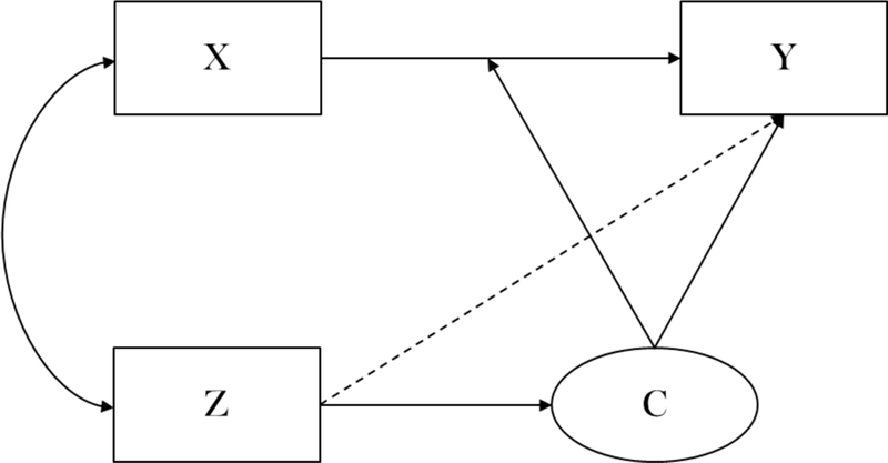
Path diagram of a regression mixture model with X predicting outcome Y and covariate Z predicting latent class membership C

where k denotes the given class, β_0k is the intercept for class k, β_1k is the class-specific regression coefficient that captures the differential effect of predictor x on the outcome y across latent classes, β₂ is the effect of class predictor on the outcome (dotted line in Figure 1), and σ²_k is the residual variance for class k. Individual cases are assigned to latent classes using a multinomial equation as a function of the overall latent class probabilities and potentially also as a function of the latent class predictor, z:

$$\mathrm{Pr}\left(c_i=k\text{|}{z}_i\right)=\frac{\text{exp}\left({\alpha }_k+{\gamma }_k{z}_i\right)}{{{\displaystyle \sum }}_{s=1}^K\text{exp}\left({\alpha }_s+{\gamma }_s{z}_i\right)},$$ [eq. 2]

where α_k is the log odds of being in class k versus the reference class when all covariates, z, equal zero, γ_k is the class-specific effect of z. Z acts as an explanatory variable, predicting latent class membership and therefore also explaining the heterogeneity in regression weights captured by latent classes. For simplicity this model includes single variables for x, z, and y, and this can be extended to include multiple variables in each role.

Introducing latent class predictors in Mixture Models.

There have been a number of papers debating the process of introducing latent class predictors in the framework of latent class analysis and growth mixture modeling (Asparouhov & Muthén, 2014; Bakk, Tekle, & Vermunt, 2013; D. Huang, Brecht, Hara, & Hser, 2010; G.-H. Huang & Bandeen-Roche, 2004; Li & Hser, 2011; Lubke & Muthén, 2007; B. O. Muthén, 2004; Vermunt, 2010). Vermunt (2010) outlines two distinct methods: a one-step estimation method and a stepwise (three-step) estimation method. In the one-step approach, latent classes are estimated jointly with their predictors in one overall model. Therefore, the predictors of the latent classes help to define each latent class. In contrast, the three-step approach involves first identifying the latent classes based only on their indicators without the class predictor(s). In the second step, participants’ posterior membership probabilities from the first step are used to create the most likely class membership. In the third step, the most likely class variable is then used as an outcome variable and regressed on the latent class predictor variables while adjusting for the uncertainty in class assignments (Asparouhov & Muthén, 2014; Bakk et al., 2013; Vermunt, 2010).

While some studies argue that the one-step approach results in more reliable parameter estimates (Asparouhov & Muthén, 2014), other studies argue that the three-step approach (Bakk et al., 2013; Vermunt, 2010) more closely follows the logic of the typical latent class analyses. The reasoning for the one-step approach, which involves estimating the full model, is that it includes the most information because latent class predictors are allowed to assist with classification. Thus, using this approach should improve class enumeration and reduce standard errors (Clark & Muthén, 2009). However, inclusion of class predictors in one step greatly increases the number of parameters possible in the model, which increases the chances of any model misspecifications associated with the latent class predictors. The rationale for the three-step approach is that the class predictors are kept distinct from the classes themselves thus they do not change the interpretation of the classes and no explicit assumptions about class predictors are made. Because many researchers view class predictors as logically being introduced after a classification model has been built, the classification model and the predictor model are developed separately in many research studies, which map on to the three-step approach (Liu & Lu, 2011, 2012; Wong & Maffini, 2011; Wong et al., 2012). One of the benefits of using the three-step approach over the one-step approach is that the classification model does not make assumptions about class predictors. In other words, class enumeration, which is accomplished at the first step, should not be affected by any model misspecifications associated with a latent class predictor. On the other hand, because the classification model and the predictor model are separately analyzed, the three-step approach does assume no direct relationship between the latent class predictor and the outcome variable.

Omitted direct effect of latent class predictors on outcomes.

In practice it is common to assume that class predictors are unrelated to outcomes (Ding, 2006; Liu & Lu, 2011, 2012; Schmeige, Levin, & Bryan, 2009). Asparouhov and Muthén (2014) conducted a simulation study to examine the effects of omitted direct effects on the three-step estimation in the context of latent class analysis (LCA) and growth mixture models. They compared three approaches: a three-step approach excluding direct effects, a three-step approach including direct effects, and a one-step approach including direct effects. The three-step approach including direct effects was conducted by adding the covariate at step 1 to account for the direct covariate effect on the class indicator variables while the covariate effect on the class probability is still analyzed at step 3. They found that the three-step approach omitting the direct effects performed poorly showing substantial bias in regression weights. The three-step approach including the direct effects performed better than the one without the direct effect in the model, but the biases substantially increased when the number of direct effects was large and the class separation was low (i.e., entropy < 0.6). In this case the one-step approach outperformed the other two alternatives, which was expected given that the datasets were generated based on the one-step approach. In their study, however, the one-step approach omitting the direct effects was not examined because the focus of the study was on the three-step estimation method.

Class separation in regression mixture models.

As shown in previous studies, low class separation indicated by low entropy has a large impact on results of the mixture model (Bakk, Oberski, & Vermunt, 2014; Bakk et al., 2013; Lubke & Muthén, 2007; Park, Lord, & Hart, 2010; Vermunt, 2010). Entropy is a measure of classification accuracy expressed as

$$E_k=1-\frac{{\sum }_i{\sum }_k(-{\widehat{p}}_{ik}\ln {\widehat{p}}_{ik})}{n\ln k},$$

where n is the sample size, k is the number of latent classes, and ${\widehat{p}}_{ik}$ denotes the estimated conditional probability for individual i in class k. Entropy is scaled to be 1 indicating perfect classification while 0 indicating chance classification (Ramaswamy, DeSarbo, Reibstein, & Robinson, 1993). Although there may be also differences in intercept and residuals, when latent classes are separated primarily by differences in regression weights, many observations do not clearly belong to one class which leads to low entropy. As Van Horn et al. (2014) showed, low entropy is typical in regression mixtures and is not an indicator of model misfit. Assigning individuals to classes using most likely class membership with poor class separation and low entropy can cause a problem for estimating the covariate effects in three-step approach (Bakk et al., 2013; Vermunt, 2010). Although the three-step approach provides an adjustment for classification error by fixing the class proportion, it still requires a certain level of classification accuracy and the quality of results has been shown to decrease along with entropy (Bakk et al., 2014).

Direct covariate effect in Regression Mixture Model.

We believe that the issues which arise when including predictors of class membership are more complex in regression mixture models than in other mixture models and that the topic warrants a separate evaluation. Besides the impact of typically low entropy in regression mixtures on the performance of the 3-step model, low entropy also results in less stable model solutions such that each model assumption and parameter can impact the substantive conclusions (George, Yang, Jaki, et al., 2013; George, Yang, Van Horn, et al., 2013; Kim et al., In press; Van Horn et al., 2012). Failure to model important parameters has been shown to bias model results (Kim et al., In press), but additional model complexity from including unneeded parameters may also hurt model performance in terms of the reduced power. Additionally, unlike LCA in which latent classes are identified using the assumption of local independence, latent classes in regression mixtures are identified based on the assumptions made about the conditional distribution of error terms.

Because we believe that regression mixtures are substantively different from other mixture models in this regard, we focus our review of the inclusion covariates on studies which used regression mixtures. In his demonstration of the application of regression mixtures in educational research, Ding (2006) included two predictors of the latent class (i.e., gender and race) and apparently did not model the direct effects of covariates on the outcome. Liu and Lu (2012) employed regression mixture models to examine the differential effect of students’ academic stress on depressive symptoms including gender and school climate as latent class predictors in the model. While testing the effects of two covariates on the latent class membership, the direct covariate effects on the outcome were not reported in the results of the study. Likewise, Schmeige et al. (2009) did not mention testing this direct effect when using regression mixture models to examine the heterogeneity in the effect of risky sexual behavior on alcohol use among criminally-involved adolescents. Of the applied regression mixture models which examine predictors of latent classes, Van Horn et al.’s study (2009) only appears to have modeled direct effects of the covariates. We found no previous study that specifically examined approaches to including predictors of latent classes in regression mixtures.

Study aims

The purpose of the current study is to provide guidance on a process for including latent class predictors in regression mixture models. One of the common assumptions made in this process is that there is no direct effect of the latent class predictor on the outcome variable. The first goal of this study is to examine the impact of omitting the direct effect on class enumeration and parameter estimates in generally used one-step and three-step estimation approaches. We estimate four different models: (1) the one-step approach including the direct effect, (2) the one-step model excluding the direct effect, (3) the three-step approach excluding the direct effect, and (4) the three-step approach including the direct effect.

First, we analyze the most general one-step approach including the direct effect to validate the data-generating process; we expect no bias in class enumeration and the parameter estimates. Next, we examine the effect of omitting the direct effect in the one-step approach. We expect too many latent classes will be identified because additional classes will be required to fit the data due to the omitted direct effect. Third, we examine the effect of omitting the direct effect in the three-step approach. We followed the three-step approach by Vermunt (2010), which starts with the classification model at step 1, classifies individuals using highest posterior probabilities at step 2, and assesses the covariate effect on the latent classes at step 3. As in most uses of the 3-step approach, the direct effect of latent class predictor on the outcome variable is omitted at step 1. We expect class enumeration to show minimal bias because the latent classes are solely determined by the effect heterogeneity. However, when the latent class predictor and the predictor with differential effects are correlated, regression weights should be overestimated because the ignored direct effect will be attributed to the predictor variable. The covariate effect on the latent class membership is expected to be overestimated because the direct relationship between the covariate and outcome is not taken into account. Last, we examine the performance of the adjusted three-step approach proposed by Asparouhov and Muthen (2014) by including the direct covariate effect on the latent class indicator at the first step. We hypothesize that when there is a covariate effect on the latent class, class enumeration will still show minimal bias. However, the parameter estimates for the direct covariate effect will be overestimated due to the failure to model the covariate effect on the latent class. We also expect that both 3-step approaches will show less stable results because of the problems using this approach with weak class separation.

Our second goal is to show the model building process for including a latent class predictor in regression mixture models in an applied dataset. First, we analyze an ‘unconditional model’ which includes no latent class predictors and thus where the focus of the model is on differences between classes in regression weights. Next, we then bring the latent class predictors into the unconditional model and examine substantive differences in the model results. We do not focus on a formal test for whether the models are different or not, in practice it is nearly always the case that model results change. The important question is whether the class predictors substantively change the interpretation of the results such that the same differential effects are not observed. This proposed method would be problematic if exclusion of a latent class predictor presents substantial bias in class enumeration when there actually is a significant effect in a population model. Asparouhov and Muthen (2014) argue that this may be the case in LCA, but it is not clear that this would typically be the case in regression mixtures. Finally, we use an applied dataset to show the effects of omitting the direct effect from the latent class predictors to an outcome variable.

Methods: Simulation Study

Data generation.

This study uses Monte Carlo simulations to examine the impact of the omitted direct effect of a latent class predictor in regression mixtures. We generated data using R (R Development Core Team, 2010) for a 2-class model as a true population model. Two different regression weights (i.e., β₁₀ = 0.20 for small effect group and β₂₀ = 0.70 for large effect group) were used for generating the data for each class. We adopt these regression weights for this simulation study because we believe that if the model cannot capture a difference in effect sizes of at least this large (the difference between a small and a large correlation), it is of limited use in capturing the differential effect of x on y. While holding the regression weights constant for the two classes across simulation conditions, we manipulated the degree of direct effect (y on z; 0 and 0.50), covariate effect (c on z; odds ratio of 1, 2, and 3), and correlation between x and z (0 and 0.50). Thus, a total of 12 separate conditions (2 X 3 X 2) with 500 replications for each model are used to generate the data using the following equations:

$${\text{y}}_{\text{i|c=1}}\text{=0}.0+0{\text{.20x}}_{\text{i}}\text{+}\left[\begin{array}{c}\text{0}\\ \text{0}.50\end{array}\right]{\text{z}}_{\text{i}}{\text{+e}}_{\text{i}}~N\left(0,.96\right),$$

$${\text{y}}_{\text{i|c=2}}\text{=0}.5+0{\text{.70x}}_{\text{i}}\text{+}\left[\begin{array}{c}\text{0}\\ \text{0}.50\end{array}\right]{\text{z}}_{\text{i}}{\text{+e}}_{\text{i}}~N\left(0,.51\right),$$

$$\text{Pr}\left({\text{c}}_{\text{i}}{\text{=k|z}}_{\text{i}}\right)\text{=}\frac{\text{exp(0}.0+\left[\begin{array}{c}\text{0}\\ \text{0}.69\\ \text{1}.12\end{array}\right]{\text{z}}_{\text{i}}\text{)}}{\text{1+exp(0}.0+\left[\begin{array}{c}\text{0}\\ \text{0}.69\\ \text{1}.12\end{array}\right]{\text{z}}_{\text{i}})}.$$

Although previous studies showed that regression mixture models are sensitive to non-normal errors (Van Horn et al., 2009), we only considered normally distributed residual variances in this study because normality is beyond the scope of this paper. Entropy is not manipulated in the study because changing entropy requires changing the effect sizes and the variance components, which precludes comparing model results across all simulation conditions. Given that entropy is a function of conditional probability given the number of subjects and classes, it is changed depending upon the effect of latent class predictor (C on z), class differences in intercepts, and class specific residuals. We chose a sample size of 3000 for each class with a total of 6000 in each dataset because regression mixture models are considered as a large sample method (Fagan, Van Horn, Hawkins, & Jaki, 2012; Van Horn et al., 2009) and samples of this size are available in many publicly available datasets. Sample R code for generating the dataset is included in the Appendix.

Data analysis.

Mplus 7.1 (L. K. Muthén & Muthén, 1998–2012) employing the maximum likelihood estimator with robust standard errors (ESTIMATOR=MLR) was used for estimating the regression mixture models. Four types of regression mixture models were analyzed to investigate the optimal strategy for including the latent class predictor(s) in the model: (1) correctly specified one-step model, (2) omitting the direct effect of y on z in one-step model, (3) three-step approach excluding the direct effect of y on z (4) adjusted three-step approach including the direct effect of y on z at step 1. The class-specific residual variances are estimated for all four approaches given that a previous study show that equality constraint on the residual variances across classes has a substantial impact on the bias in class enumeration and parameter estimates (Kim et al., In press). Determining the appropriate number of latent classes is the first step of estimating a regression mixture model, which involves testing a series of models with an increasing number of latent classes in order to assess the fit of the model. For each type of model specification, we started with a traditional regression model (i.e., 1-class model) followed by adding one more class into the model. Given that the true population model was a 2-class model, we analyzed a model with 1, 2, and 3 classes. Additionally, we analyzed a model with 4 and 5 classes for some simulation conditions to examine the degree of bias in class enumeration when 3-class model was selected in majority of simulations. If a 5-class model showed better model fit than a 4-class model, we stopped adding more classes and concluded that the model selected too many classes. Latent class enumeration is based on the Bayesian information criterion (BIC; Schwarz, 1978) and the sample size adjusted BIC (aBIC; Sclove, 1987). Better model fit is indicated by smaller values in BIC and aBIC. Because previous literatures in regression mixture models have shown that Akaike Information Criteria (AIC; Akaike, 1974) is likely to select too many classes, we have not considered using the AIC in this study; see (Nylund, Asparauhov, & Muthen, 2007; Van Horn et al., 2009) for further discussion.

Following class enumeration, we also assessed the accuracy of parameter estimates in all four approaches. Because of the label switching problem in latent class analysis (McLachlan & Peel, 2000; Sperrin, Jaki, & Wit, 2010; Tueller, Drotar, & Lubke, 2011), we first sorted the two classes by the slope coefficients so that the smaller effect size class was always labeled as Class-1 and the larger effect size class to be Class-2. To assess the accuracy of the estimated parameters, we present the average parameter estimates and the standard deviation of the parameter estimates across all 500 simulations. Among all the estimated parameters, we focus on the regression weights (intercepts and slopes) for the two classes (i.e., β₀₀, β₀₁, β₁₀ and β₁₁) and the covariate effect on the class membership (γ₀). For the adjusted three-step approach, we also assess the accuracy of the direct effect (i.e., β₂), which is estimated at the first step.

Results: Simulation Study

Class enumeration.

All models with 1 and 2 classes converged while the convergence rate for the 3-class model ranged from 96% to 100% across all simulation conditions. The true population value for entropy was estimated using a single simulation from a dataset with 100,000 subjects generated and analyzed using a 2-class regression mixture model. The estimated entropy values for the correctly specified model are given in Table 1. As expected, entropy under the current study setting are very low. Table 1 shows the class enumeration results for four different model specifications across 12 simulation conditions in terms of the covariate effect (C on z), correlation between the predictor variables (x with z), and direct covariate effect on outcome (y on z). First, the one-step approach including the direct effect shows that the true 2-class model is selected in nearly all simulations using both the BIC and aBIC, indicating that the data are properly generated. Second, when omitting the direct effect in the one-step approach, class enumeration results are severely biased. As shown in Table 1, if there is no relationship between the class predictor and the outcome (β₂ = 0; condition 1, 2, 5, 6, 9, and 10) regardless of the correlation between X and z and the covariate effect on class membership (C on z), the 2-class model is correctly selected in most simulations. However, once there is a direct effect of y on z (β₂ = 0.5; condition 3, 4, 7, 8, 11, and 12), the 2-class model is not properly captured, but the 3-class model is always selected over the true 2-class model. To further examine the effect of the omitted direct effect in class enumeration, we analyzed additional models with 4 and 5 classes for all 500 simulations for each condition¹. Results showed that multiple additional classes were required to account for the omitted direct covariate effect on the outcome with the aBIC typically selecting 5 or more classes and the BIC usually indicating 4 or more classes.

Table 1.

Class enumeration results for four model specifications.

Study conditions					Model specification
No.	C on z	x with z	y on z	Entropya	True (1-step)		Omit y on z (1-step)		Omit z (3-step)		Adjusted 3-step
					BIC	ABIC	BIC	ABIC	BIC	ABIC	BIC	ABIC
1	0	0	0	.127	100.0%	98.8%	100.0%	99.2%	100.0%	97.4%	100.0%	98.6%
2	0	.5	0	.128	100.0%	99.2%	100.0%	99.4%	100.0%	99.0%	100.0%	98.8%
3	0	0	.5	.129	100.0%	99.0%	0.0%	0.0%	99.8%	97.4%	99.8%	97.8%
4	0	.5	.5	.135	100.0%	99.2%	0.0%	0.0%	100.0%	98.2%	99.8%	97.6%
5	−.69	0	0	.189	100.0%	99.4%	100.0%	99.4%	100.0%	97.8%	100.0%	97.6%
6	−.69	.5	0	.210	100.0%	98.7%	100.0%	99.4%	99.8%	96.2%	100.0%	97.0%
7	−.69	0	.5	.192	100.0%	98.8%	0.0%	0.0%	99.8%	98.4%	99.6%	98.0%
8	−.69	.5	.5	.198	100.0%	98.6%	0.0%	0.0%	100.0%	98.6%	100.0%	97.8%
9	−1.1	0	0	.264	100.0%	99.0%	100.0%	99.4%	100.0%	98.6%	100.0%	97.8%
10	−1.1	.5	0	.296	100.0%	98.4%	100.0%	98.6%	99.4%	94.6%	99.8%	93.8%
11	−1.1	0	.5	.264	100.0%	98.6%	0.0%	0.0%	100.0%	98.0%	100.0%	98.8%
12	−1.1	.5	.5	.287	100.0%	98.7%	0.0%	0.0%	100.0%	97.2%	100.0%	94.8%

^aNote.N=100,000 was used to obtain the entropy value.

In the three-step approach, the number of latent classes is determined at the first step, which uses the unconditional model excluding the latent class predictor z. As shown in Table 1, excluding the covariates has no serious impact on the latent class enumeration in both traditional three-step approach (omitting the direct effect) and the adjusted three-step approach (including the direct effect). As we expected, class enumeration is robust to excluding the class predictor from the model. When omitting the direct effect, the true two classes are selected using the BIC in above 99% of simulations and the aBIC in 96% or above. When including the direct effect, the detection rates are above 99% using the BIC and above 93% using the aBIC across all simulation conditions.

Accuracy of parameter estimates.

To ensure that the data generating process was proper, we first analyzed the correctly specified 1-step approach including the direct effect and confirmed that there was no bias in parameter estimates². The accuracy of the parameter estimates from the 2-class model are assessed using the mean (M) and the standard deviation (SD) of the parameter estimates across 500 simulations. Table 2 presents the parameter estimates for the class-specific intercepts (β₀₀ and β₀₁) and slopes (β₁₀ and β₁₁), direct covariate effect on the outcome y (β₂), covariate effect on the class probability (γ₀), and the intercept of the class probability (α₀) when omitting the direct effect y on z in the 1-step approach. As shown in Table 2, we found no bias in the estimated parameters when there was no direct effect in the population model (β₂ = 0; condition 1, 2, 5, 6, 9, and 10) as we had no problem in class enumeration. This is reasonable given that the model is appropriately specified; constraining the y on z path to be zero is identical with omitting the corresponding path. When a moderate direct effect is omitted in the one-step approach, however, bias in the estimated parameters is substantial (see Table 2; condition 3, 4, 7, 8, 11, and 12). The intercept differences between the two classes are substantially overestimated and the regression weights for Class-1 are substantially overestimated while the weights for Class-2 are underestimated, which leads to get no clear differences in regression weights between classes. Thus the interpretation of the results changes substantially when the direct effect is omitted. The latent classes are mainly differentiated by the intercept differences not the regression weights. Next, the covariate effect on class probability (C on z; γ₀) is also biased when the moderate direct effect is omitted. Results consistently show that the covariate effect is increased under all six conditions in which the moderate direct effect is omitted, which indicates that the omitted direct effect of y on z is carried through the indirect effect of C on z. Bias in the estimated covariate effect is larger when the predictor x is not correlated with the latent class predictor z.

Table 2.

Parameter estimates when omitting the direct effect in the 1-step approach

Study conditions				Estimated parameters
No.	C on z	x with z	y on z	Class 1				Class 2				C on z (γ0)		Int.Prob (α0)
				Intercept (β00=.00)		Slope (β10=.20)		Intercept (β01=.50)		Slope (β11=.70)
1	0	0	0	−.01	(.05)	.20	(.04)	.50	(.04)	.70	(.03)	.00	(.07)	−.02	(.25)
2	0	.5	0	.00	(.05)	.20	(.04)	.50	(.04)	.70	(.03)	.01	(.06)	.02	(.24)
3	0	0	.5	−.36	(.04)	.40	(.02)	.88	(.04)	.51	(.02)	−2.29	(.12)	.07	(.19)
4	0	.5	.5	−.39	(.07)	.48	(.02)	.88	(.07)	.59	(.02)	−2.03	(.24)	.06	(.19)
5	−.69	0	0	.00	(.04)	.20	(.04)	.50	(.03)	.70	(.03)	−.71	(.09)	.00	(.20)
6	−.69	.5	0	−.01	(.04)	.20	(.04)	.50	(.03)	.70	(.03)	−.70	(.08)	.00	(.21)
7	−.69	0	.5	−.42	(.04)	.34	(.02)	.92	(.03)	.57	(.02)	−2.57	(.13)	−.01	(.17)
8	−.69	.5	.5	−.38	(.04)	.44	(.02)	.98	(.03)	.69	(.02)	−2.37	(.12)	.28	(.18)
9	−1.1	0	0	.00	(.04)	.20	(.03)	.50	(.02)	.70	(.02)	−1.12	(.12)	.02	(.19)
10	−1.1	.5	0	.00	(.04)	.20	(.03)	.50	(.03)	.70	(.02)	−1.11	(.11)	.01	(.20)
11	−1.1	0	.5	−.44	(.04)	.31	(.02)	.94	(.03)	.59	(.02)	−2.80	(.14)	−.03	(.17)
12	−1.1	.5	.5	−.39	(.04)	.42	(.02)	1.00	(.03)	.72	(.02)	−2.64	(.13)	.30	(.18)

To ease the understanding of substantive changes in differential effects, we present example density plots when omitting the direct covariate effect. Figure 2 presents the density plots for the differences in slope coefficients from the 2-class models when omitting the direct effect of y on z. The two top panels in Figure 2 show that the two classes were well separated with the peak around the true population values (β₁₀ = .20 and β₁₁ = .70) for condition 5 and 6, which has no direct effect (β₂ = 0). The bottom two panels in Figure 2 show the density of the two regression weights when omitting the direct effect under the moderate covariate effect. Effects of misspecification are seen in regression weights for each class, which are shifted towards each other. We note that the class assignment strategy (i.e., the smaller effect was assigned to be Class-1 in every simulation) means that these results are overly optimistic. Class enumeration results support this argument because in many cases the true two classes are not selected but more number of classes are selected over the 2-class model.

Figure 2.

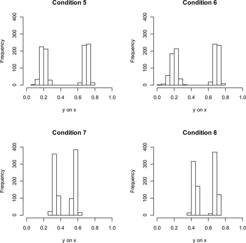
Slope coefficients (y on x) of two classes when omitting the direct covariate effect in 1- step approach

Next, Table 3 presents the parameter estimates when omitting z from the first step of the three-step approach. In the table, class-specific intercepts and slopes are obtained from the first step while the covariate effect (γ₀) is estimated at step 3. Class-specific intercept coefficients (true β₀₀=0.0 and β₀₁=0.5) are adequately estimated in most conditions except when there is at least a moderate covariate effect and the direct effect. For condition 7, 8, 11, and 12, intercept coefficients for Class-1 are underestimated (ranged −0.17 to −0.33) while those for Class-2 are overestimated (ranged 0.61 to 0.72), which makes the intercept differences between the two classes to be larger than the true value. On the other hand, we have found no bias in the regression weights (slope coefficients) except for the condition 4, 8, and 12, which contains a moderate correlation between x and z. When the latent class predictor is moderately related to the covariate (r_xz = 0.5), the regression coefficients are substantially overestimated for both classes when omitting the direct effect. This is expected because the direct and indirect (through the class membership) effect of the covariate z should be carried through the predictor x. Although parameters are upwardly biased, the difference in the regression weights and the substantive interpretation of the latent classes is still properly captured by the three-step approach unlike the case with the direct effect in the one-step approach omitted. On the other hand, the class mean at step 1 (true α₀=0.0), which is the probability of being assigned to be in Class-1, is biased when there is at least a moderate covariate effect and a correlation between x and z. For condition 6, 8, 10, and 12, the class mean is underestimated (ranged −0.26 to −0.54) indicating that more subjects are assigned to be in Class-2.

Table 3.

Parameter estimates from the traditional three-step approach

Study conditions				Estimated parameters
No.	C on z	x with z	y on z	Class 1				Class 2				Step-1		Step-3
				Intercept (β00=.00)		Slope (β10=.20)		Intercept (β01=.50)		Slope (β11=.70)		Class mean (α0=.00)		C on z (γ0)		Int.Prob (α0=.00)
1	0	0	0	−.01	(.05)	.20	(.04)	.50	(.04)	.70	(.03)	−.02	(.25)	−.02	(.25)	−.01	(.08)
2	0	.5	0	.00	(.05)	.20	(.04)	.50	(.04)	.70	(.03)	.02	(.24)	.07	(.41)	.02	(.27)
3	0	0	.5	−.03	(.11)	.19	(.06)	.50	(.06)	.70	(.06)	−.07	(.43)	−2.73	(.65)	−.46	(.77)
4a	0	.5	.5	−.02	(.09)	.45	(.06)	.51	(.06)	.95	(.05)	−.02	(.42)	−2.53	(2.20)	.51	(1.46)
5	−.69	0	0	.00	(.05)	.20	(.04)	.50	(.04)	.70	(.03)	.00	(.23)	−.70	(.12)	.00	(.25)
6	−.69	.5	0	.02	(.07)	.20	(.06)	.48	(.03)	.69	(.03)	−.26	(.30)	−.40	(.34)	−.25	(.35)
7	−.69	0	.5	−.17	(.10)	.20	(.05)	.66	(.05)	.70	(.04)	−.02	(.29)	−3.73	(.50)	−.26	(.62)
8	−.69	.5	.5	−.20	(.17)	.44	(.06)	.61	(.05)	.93	(.05)	−.38	(.38)	−2.16	(.75)	−.45	(.64)
9	−1.1	0	0	.00	(.05)	.20	(.04)	.50	(.03)	.70	(.03)	.01	(.26)	−1.09	(.16)	.01	(.30)
10	−1.1	.5	0	.04	(.10)	.20	(.07)	.47	(.04)	.69	(.03)	−.37	(.34)	−.70	(.32)	−.37	(.40)
11	−1.1	0	.5	−.24	(.09)	.20	(.04)	.72	(.05)	.70	(.04)	−.01	(.24)	−3.89	(.43)	−.18	(.54)
12	−1.1	.5	.5	−.33	(.24)	.45	(.07)	.64	(.05)	.91	(.05)	−.54	(.42)	−2.29	(.64)	−.73	(.66)

^aNote.Three cases with extreme value for the C on z class probability (< −10) are excluded from calculating the mean of the parameter estimates.

While class differences in regression weights are recovered relatively well using the three-step approach, we found substantial bias in the effect of the latent class predictor on the class probability, γ₀. As shown in Table 3, the covariate effect is properly estimated only when there is no direct effect and zero correlation of x with z. Even when there is no direct covariate effect (true β₂=0), the indirect covariate effect (C on z) tends to be affected by excluding the covariate z from the model if there is a correlation between the predictor x and covariate z. For condition 6 and 10, the covariate effect (γ₀) is underestimated while sampling variability is increased. When there truly is a moderate direct effect and it is omitted (condition 3, 4, 7, 8, 11, and 12), bias in the indirect covariate effect is substantially increased with larger sampling variability. For condition 4, especially, we observe an extreme value of C on z in some simulations (see footnote in Table 3), indicating unstable results of the three-step approach. We excluded the extreme values (i.e., absolute value above 10) in calculating the mean and standard deviations of γ₀ in that condition. Even after excluding the extreme cases, results show that the covariate effect is severely biased with substantial sampling variability.

Last, Table 4 presents the parameter estimates when including the direct effect in the three-step approach following the adjustment proposed by Asparouhov and Muthen (2014). In this adjusted approach, the latent class predictor z is included in the first step to take into account the direct relationship between the class predictor and the outcome variable. Thus in Table 4, class-specific intercepts (β₀₀, β₀₁) and slope coefficients (β₁₀, β₁₁) and the direct effect (β₂) are obtained from step 1 while the covariate effect (γ₀) is estimated at step 3. As shown in results, although the regression weights for the two latent classes are slightly overestimated when there is a relationship of x with z (condition 6, 8, 10, and 12), they are relatively well estimated and the magnitude of differential effects are captured adequately across all simulation conditions. The direct effect of y on z obtained in step 1 appears to suffer primarily from increased sampling variability. Next, the primary focus of this paper, the covariate effect (C on z) obtained from step 3 in this case, shows bias in almost all scenarios except when the covariate is not related with the class membership as well as the predictor x. The covariate effect is slightly overestimated when there actually is no effect on the class probability but there is a correlation between x and z (condition 2 and 4). The sampling variability is noticeably increased under these conditions. When there is a moderate (γ₀=.69) or a large (γ₀=1.10) covariate effect, which corresponds to the odds ratio of 2 and 3 respectively, the covariate effect is underestimated in all simulation conditions (condition 5 through 12). Bias increases when the predictor x is related with the latent class predictor z, and sampling variability is substantial when the latent class predictor z is correlated with x.

Table 4.

Parameter estimates from the adjusted three-step approach including the direct covariate effect at step-1

Study conditions				Estimated parameters
No.	C on z	x with z	y on z	Class 1				Class 2				Step-1				Step-3
				Intercept (β00=.00)		Slope (β10=.20)		Intercept (β01=.50)		Slope (β11=.70)		Class mean (α0=.00)		y on z (β2)		C on z (γ0)		Int. Prob (α0=.00)
1	0	0	0	.01	(.05)	.20	(.04)	.50	(.04)	.70	(.03)	−.02	(.25)	.00	(01)	−.01	(.07)	−.02	(.25)
2	0	.5	0	.00	(.05)	.20	(.04)	.50	(.04)	.70	(.03)	.02	(.24)	.00	(.01)	.07	(.41)	.02	(.27)
3	0	0	.5	−.01	(.05)	.19	(.04)	.50	(.04)	.70	(.03)	−.03	(.25)	.50	(.01)	.00	(.08)	−.03	(.25)
4	0	.5	.5	−.01	(.05)	.20	(.04)	.50	(.04)	.70	(.03)	.00	(.25)	.50	(.01)	.08	(.39)	.01	(.28)
5	−.69	0	0	.02	(.05)	.20	(.04)	.48	(.04)	.70	(.03)	.00	(.25)	.06	(.01)	−.49	(.10)	.00	(.26)
6	−.69	.5	0	.05	(.06)	.17	(.06)	.46	(.03)	.66	(.03)	−.26	(.31)	.06	(.01)	−.29	(.37)	−.25	(.36)
7	−.69	0	.5	.02	(.05)	.20	(.05)	.48	(.04)	.70	(.03)	.00	(.26)	.56	(.01)	−.48	(.11)	−.01	(.27)
8	−.69	.5	.5	.04	(.06)	.17	(.06)	.46	(.03)	.66	(.03)	−.27	(.30)	.56	(.01)	−.27	(.28)	−.27	(.32)
9	−1.1	0	0	.04	(.05)	.20	(.05)	.46	(.04)	.70	(.04)	.01	(.29)	.09	(.01)	−.77	(.15)	.01	(.31)
10	−1.1	.5	0	.09	(.10)	.16	(.07)	.44	(.03)	.65	(.04)	−.35	(.37)	.09	(.01)	−.57	(.41)	−.35	(.44)
11	−1.1	0	.5	.04	(.05)	.20	(.05)	.46	(.04)	.70	(.03)	.02	(.28)	.59	(.01)	−.77	(.16)	.01	(.31)
12a	−1.1	.5	.5	.09	(.06)	.17	(.08)	.44	(.04)	.66	(.04)	−.32	(.38)	.59	(.01)	−.64	(.62)	−.31	(.53)

^aNote.There was one extreme value (i.e., −90.03) and excluded from calculating the mean of the parameter estimates.

Conclusion: Simulation study

The simulation study shows that omitting the direct effect produces substantial bias in class enumeration in the one-step approach while it has no impact on class enumeration in either three-step approach. However, as expected given low levels of entropy, neither three-step approach adequately achieves the goal of estimating the effect of the covariate on the latent class in all scenarios. The three-step approach in which the covariate is omitted in step-1 shows adequate results for the effects of the covariate on class membership only when there is neither a direct effect of the covariate on the outcome nor a correlation between the covariate and the primary predictor (x). Otherwise the effect of the covariate on the latent class is often overestimated. The three-step approach in which the main effect of the covariate on the outcome is included in step-1 shows adequate results only when there is no effect of the covariate on the latent classes. In either case, the primary reason for utilizing a 3-step approach, to estimate the effects of covariates on latent classes, is not well served. The 1-step approach including the direct effect is the only approach, which leads to adequate estimates of the effect of the covariate on the latent classes. However, the results from step-1 of the three-step approach without the covariate suggest that it is also adequate to omit a covariate as a first step in model estimation. In this case there is no evidence of bias in class enumeration and in all cases the substantive meaning of the latent classes remains valid although when the covariate is correlated with the predictor (x), regression weights in each class are overestimated.

Model building process in regression mixtures.

The results from this simulation study suggest another option for including covariates. Given that the three-step approach shows that excluding the covariates from the step-1 has minimal impact on latent class enumeration, using the model with no covariates (i.e., unconditional model) for latent class enumeration is a reasonable first step in the model building process. It substantially reduces the amount of time needed to build an optimal model because researchers do not need to reanalyze the model whenever they include or exclude covariates. While the number of detected latent classes should be reliable for further analysis, the effect sizes for the regression coefficients are not trustworthy because the omitted covariate(s) impact estimates of regression weights. Simulations show that neither three-step method results in adequate estimates for the effects of the covariates on the latent classes.

Thus, we next suggest that once latent classes are established, the covariates should be brought into the model with the entire model re-estimated as in the 1-step approach, including the hypothesized direct effect of covariates on the outcome. The important point here is to compare the class-specific regression weights capturing effect heterogeneity from the different models. Although we expect some differences between the two results in terms of the effect sizes, the substantive meaning of the heterogeneous effects captured in the unconditional model should remain in the conditional model. Our simulations show that this approach leads to good estimates for all model parameters. The advantage of this model building process is that it gives the investigator information about whether model results are driven by the covariate. A substantial change in differential effects suggests strong covariate influence on the model or model instability and should be used as diagnostic criteria for indicating that model results need to be examined more carefully and may not valid. We also note that no evidence of a direct effect of the covariate on the outcome in the conditional model may indicate dropping that effect from the model to reduce model complexity.

Applied Example. Use of the model building process with applied data.

To demonstrate the proposed model building process for including latent class predictors in regression mixtures, we analyzed data from a previously published study, which examined heterogeneity in the effects of family resources on academic achievement (Van Horn et al., 2009). In the study, differential effects of the four types of family resources (i.e., money, basic needs, time spent-self, and time spent-family) on three student achievement outcomes (i.e., math, reading, and language) were examined taking into account the two covariates (i.e., sex and ethnicity) for model specification. This study found three latent classes – i.e., a class with the strong effect of basic needs (42%) on the academic achievement, another class being resilient to the effects of a lack of basic needs (36%), and the last class showing low academic achievement with no effect of basic needs (22%) – when including ethnicity as a covariate. The relationships of sex and ethnicity with latent classes were added after class enumeration in the unconditional model. Since this study found significant effects of sex and ethnicity on class membership (Van Horn et al., 2009), we used these two demographic variables in the current study. Male and other ethnicity students were used as the reference group for sex and ethnicity variables, respectively.

In this example, we reanalyzed the data using the model building approach proposed. We first conducted an unconditional regression mixture model, which included the predictors (i.e., four family resources) and outcomes with no covariates. Because class enumeration in the unconditional model was found to be robust to the effect of latent class predictors in the simulation study above, we decided the number of latent classes using the unconditional model. Next, we brought latent class predictors into the model with and without specific direct effects from sex and ethnicity to student achievement outcomes. We then checked for substantive changes in class enumeration and parameter estimates from the unconditional model. We also analyzed the full model, which included all possible direct effects from the latent class predictors to the outcomes, to compare the model results.

After analyzing 1- through 4- class unconditional regression mixture models (Model A in Table 5), we found three latent classes to identify the heterogeneity of the family resources on student achievement outcomes, which was similar to the findings of the previous study (Van Horn et al., 2009). Next, we included the two covariates (i.e., sex and ethnicity). We analyzed three regression mixture models, which differed in the assumptions for the direct effect from the latent class predictor(s) to the outcomes. Table 5 presents the parameter estimates from four different models: (A) an unconditional regression mixture model, (B) a model including two covariates but omitting the direct effects from the covariates to the outcomes, (C) a model including two covariates with one direct effect, and (D) a model including two covariates with all possible direct effects. Model (C) replicates the one from the original study (Van Horn et al., 2009) with respect to the direct effect of ethnicity to the outcomes are included while the direct effect of sex to the outcomes are omitted³. To present the model results, we focus on the two of the three latent classes, which show the differential effects of basic needs (i.e., strong vs. resilient) on the student achievement outcomes given that the third class is only differed by the lower intercepts. We compare the model results focusing on changes in the differential effects as a result of changing the model assumptions. We note that we do not intend to interpret all the regression coefficients in detail because the purpose of this applied example is demonstrating the model building process in regression mixtures.

Table 5.

Parameter estimates from 3-class model for applied study

Model	A. Unconditional				B. Omitting both direct effects				C. Omitting direct effect of sex				D. Full model
Class	Resilient		Basic needs		Resilient		Basic needs		Resilient		Basic needs		Resilient		Basic needs
proportion	40.90%		35.70%		49.10%		37.70%		58.70%		17.60%		64.20%		9.60%
Parameter	Coeff.	S.E.	Coeff.	S.E.	Coeff.	S.E.	Coeff.	S.E.	Coeff.	S.E.	Coeff.	S.E.	Coeff.	S.E.	Coeff.	S.E.
Reading
Intercept	488.55	.76	490.44	.58	491.48	.45	483.86	.75	489.44	.83	486.48	1.51	489.85	.77	486.49	2.82
Basic needs	−.16	.91	4.28	.92	.56	.63	1.13	38.19	−.25	.55	4.12	1.26	.00	.68	6.00	1.52
Money	2.38	.93	2.00	.79	2.06	.46	2.03	6.45	1.91	.50	1.76	1.30	1.79	.44	2.35	2.43
Time-self	−.06	.80	−.55	.71	.13	.43	−1.39	7.09	.06	.49	−1.13	1.47	.17	.40	−2.78	2.71
Time-family	−.47	.73	−2.42	.88	−1.27	.50	−.51	.90	−.90	.48	−1.70	1.30	−1.07	.40	−1.45	1.39
Math
Intercept	491.11	.71	486.52	.72	489.92	.31	484.68	.52	490.71	.75	481.91	1.24	490.99	.54	485.53	2.55
Basic needs	−.07	.63	3.37	.65	.06	.44	1.14	46.36	.22	.42	2.21	.73	.28	.48	3.00	1.74
Money	1.25	.60	1.19	.71	1.61	.36	.86	7.80	1.23	.34	1.33	1.11	1.29	.34	.92	1.72
Time-self	.48	.53	−.55	.63	.02	.35	−.57	8.58	.07	.34	−1.02	1.10	.18	.33	−1.85	1.58
Time-family	−.80	.49	−1.70	.62	−1.10	.39	−.55	.95	−.88	.36	−1.50	.94	−1.09	.32	−.65	1.26
Language
Intercept	104.70	.33	100.41	.55	105.90	.13	96.96	.38	102.34	.27	98.28	.96	102.93	.61	97.35	4.66
Basic needs	1.08	.28	3.98	.61	.53	.19	1.59	67.20	.19	.22	4.03	.98	.36	.38	5.95	1.23
Money	.63	.36	2.00	.50	.82	.18	1.34	11.33	.77	.21	1.30	.86	.79	.19	1.66	1.58
Time-self	−.25	.34	−.73	.43	−.04	.19	−1.26	12.46	−.10	.20	−1.71	.83	−.05	.19	−3.30	2.48
Time-family	−.40	.32	−2.00	.61	−.74	.20	−.55	1.25	−.49	.22	−1.26	.81	−.64	.20	−1.02	1.14

As shown in Table 5, the unconditional model (Model A) identified the two classes showing differential effects of the basic needs on the student achievement for one class having a stronger effect while the other class showing resiliency across all three outcomes. When both direct effects from sex and ethnicity to student achievement outcomes were omitted in Model (B), we found that the differential effect disappeared and the sampling variability increased substantially. To validate the class enumeration, we reanalyzed the 1-class through 4-class regression mixture models for Model (B) and found that both the BIC and aBIC selected the 4-class model as the optimal model. This indicates that the covariates strongly affect the latent class enumeration. A substantial change in the substantive differences in the effects and increased sampling variability can be an indication of model instability after introducing the covariates into the regression mixture model. In Model (C), when including just the direct effect from ethnicity to the student outcomes but omitting the direct effect of sex, the differential effect of basic needs is retained with one class showing stronger effect of basic needs on the student achievement and another class showing no significant effect of basic needs. The differential effects in Model (C) are relatively consistent with those in the unconditional model. Last, we relaxed the assumptions associated with the covariates and estimated all possible direct effects to the outcome variables (Model D). Although there are some changes in class proportions, the overall interpretation of the two latent classes remains the same with Model (A) and Model (C). The standard errors of the regression weights are relatively larger than the other two models possibly due to reduced power from the increase in number of estimated parameters.

Conclusion: Applied study

We demonstrated our proposed model building approach to including covariates using data from a previously published study. In the first step, we analyzed the unconditional regression mixture model to determine the number of latent classes in the effects of family resources on academic achievement. The 3-class model was selected as the best fitting model in which two of the three classes showed the difference in the effects of basic needs on the academic achievement. In the next step, sex and ethnicity were included as covariates to understand the characteristics of the unobserved latent classes. Results showed that the differential effect disappeared when omitting the direct effect of ethnicity on academic achievement while it was retained when omitting the direct effect of sex. This finding is supported by the original study (Van Horn et al., 2009), where boys and girls showed no difference on the number of latent classes and the overall interpretation of the classes. The current example highlights the importance of examining the relationship between the latent class predictors and the outcomes. Misspecifying the direct effect from the covariates to the outcomes can substantially change regression mixture results. Although the true model specification is not known in practice, researchers should be aware of the consequences of misspecifying the latent class predictors in regression mixtures and should compare the model results before and after including the covariates.

Discussion

There has recently been much discussion in the literature on methods for assessing the effects of covariates on latent classes (Bakk et al., 2014; D. Huang et al., 2010; Lubke & Muthén, 2007). While this literature suggests that mixtures, such as regression mixtures, which very low class separation might behave differently (Asparouhov & Muthén, 2014; Bakk et al., 2013; Li & Hser, 2011; Vermunt, 2010), until now there was no solid basis for giving advice to users of regression mixtures. Although this study tested limited simulation conditions under specific regression mixture scenario, it shows clearly that misspecifying the covariate to outcome relationship in the 1-step model can lead to dramatic problems in terms of class enumeration and parameter estimates. The alternative 3-step approaches get around the problems with class enumeration, but in general they result in bias in the effects of the covariate on the latent class, the entire purpose of including the covariate in the first place. While there are scenarios where these approaches work (and additional simulation conditions would find more or less problems), the user of these methods should be aware of the potential problems. Only the correctly specified 1-step approach led to good latent class enumeration and parameter estimates in our simulations. However, as our applied example has shown, there are also potential problems with simply estimating all possible model paths. The increased number of free parameters increases model complexity, which possibly results in larger standard error, less power, and less stable model results. We also concur with the intuitive rationale for estimating classes separately from covariates, which lies behind the 3-step approach.

Our conclusion is that there is no simple ‘one size fits all’ solution to how to include predictors of latent classes in regression mixtures. Rather, we recommend a model building process where the model is first estimated with no predictors of latent classes. Once a stable solution for class enumeration has been obtained, class predictors are then brought into the model with a fixed number of latent classes and their effects on parameter estimates and possibly class enumeration is examined. When covariates are brought into the model, it is important that the direct effects of the covariates on the outcome are considered as well. This will prevent the solution being dominated by possibly false assumptions about the latent class predictors. Additionally, this model building process has diagnostic value; when results change substantially by including covariates into the model, then the model should be reexamined. While not tested in this paper, there is no obvious reason why this model building approach to adding covariates would not be successful for other mixture models as well. For many mixtures a 3-step approach performs quite well, however, the 3-step approach still assumes that there is no direct effect of the covariates on the class indicators. Testing this assumption by bringing covariates into the model and looking for substantive changes in results as well as evidence of direct effects is good practice and has value as a tool for checking the stability and sensitivity of model results.

One viable approach to deciding which direct effects of the covariates should be included in the mixture model is using residual statistics, such as, bivariate residual (BVR; Magidson & Vermunt, 2001) and expected parameter change measure (EPC; Oberski & Vermunt, 2014), which can be requested in most SEM based statistical software (e.g., LatentGold, Mplus, and LISREL). BVR is a fit index measuring the degree to which the bivariate cross-table between a pair of observed variables fit the model (Vermunt & Magidson, 2013), which can detect a local dependence. Based on the value of BVR, the omitted direct effects can be brought back into the model to increase the model fit (Oberski, 2015). Similarly, EPC is a measure for detecting local dependencies in latent class models (Oberski & Vermunt, 2014). EPC shows the change in parameter estimates when freely estimating a corresponding model component in the alternative model. Although the use of both BVR and EPC have been suggested for detecting local dependence in latent class analysis, they should perform in a similar manner in regression mixtures to guide the direct covariate effects.

This study has some significant limitations, the most important of which is that, like any simulation study, we look at a relatively small set of the possible regression mixtures models. While we do not know how many different situations these results generalize to, we believe that the finding that a misspecified 1-step approach as well as both 3-step approaches currently in the literature can fail dramatically under certain conditions is important. The fact that this can happen means that investigators should check their results to confirm that it did not happen in their case. Given that there are straightforward ways to check the results, we believe that our primary conclusions hold even though they are based on a limited set of simulations. Another limitation in the process we have suggested is that it is quite subjective. We expect that parameter estimates will change when covariates are included in the model. We have made the distinction between substantive changes which change the model interpretation and those which simply move parameter estimates. However, this distinction is arbitrary and subject to interpretation by the investigator. Given that we expect some changes more than just chance, we do not believe that a statistical test for differences is appropriate. Probably the most reasonable approach to this problem is to assure that all results are reported so that readers can determine on their own whether they agree with results. Finally, our simulations did not stress the model at all, especially with regards to distributional assumptions. In real data, none of these problems occur in isolation and it is likely that factors such as the direct effect of covariates, distributional assumptions, assumptions about linearity, and sample size interact. Future research to assess these interactions would be very interesting although also incredibly difficult.

References

- Akaike H (1974). A new look at the statistical model identification. IEEE Transactions on Automatic Control, 19, 716–723. [Google Scholar]
- Asparouhov T, & Muthén B (2014). Auxiliary Variables in Mixture Modeling: Three-Step Approaches Using M plus. Structural Equation Modeling: A Multidisciplinary Journal, 21(3), 329–341. [Google Scholar]
- Bakk Z, Oberski DL, & Vermunt JK (2014). Relating latent class assignments to external variables: standard errors for correct inference. Political analysis, mpu003. [Google Scholar]
- Bakk Z, Tekle FB, & Vermunt JK (2013). Estimating the association between latent class membership and external variables using bias-adjusted three-step approaches. Sociological methodology, 43(1), 272–311. [Google Scholar]
- Clark SL, & Muthén B (2009). Relating latent class analysis results to variables not included in the analysis. Submitted for publication. [Google Scholar]
- Desarbo WS, Jedidi K, & Sinha I (2001). Customer value analysis in a heterogeneous market. Strategic Management Journal, 22, 845–857. [Google Scholar]
- Ding C (2006). Using Regression Mixture Analysis in Educational Research. Practical Assessment Research & Evaluation, 11(11). [Google Scholar]
- Fagan AA, Van Horn ML, Hawkins JD, & Jaki T (2013). Differential effects of parental controls on adolescent substance use: For whom is the family most important? Journal of quantitative criminology, 29(3), 347–368. [DOI] [PMC free article] [PubMed] [Google Scholar]
- George MRW, Yang N, Jaki T, Feaster DJ, Smith J, & Van Horn ML (2013). Finite mixtures for simultaneously modeling differential effects and nonnormal distributions. Multivariate Behavioral Research, 48(6), 816–844. [DOI] [PMC free article] [PubMed] [Google Scholar]
- George MRW, Yang N, Van Horn ML, Smith J, Jaki T, Feaster DJ, & Maysn K (2013). Using regression mixture models with non-normal data: Examining an ordered polytomous approach. Journal of Statistical Computation and Simulation, 83(4), 757–770. [DOI] [PMC free article] [PubMed] [Google Scholar]
- Huang D, Brecht M-L, Hara M, & Hser Y-I (2010). Influences of covariates on growth mixture modeling. Journal of drug issues, 40(1), 173–194. [DOI] [PMC free article] [PubMed] [Google Scholar]
- Huang G-H, & Bandeen-Roche K (2004). Building an identifiable latent class model with covariate effects on underlying and measured variables. Psychometrika, 69(1), 5–32. [Google Scholar]
- Kim M, Lamont A, Jaki T, Feaster DJ, George H, & Van Horn L (In press). Impact of an equality constraint on the class-specific residual variances in regression mixtures: A monte carlo simulation study. Behavior Researh Methods. [DOI] [PMC free article] [PubMed] [Google Scholar]
- Li LB, & Hser Y-I (2011). On inclusion of covariates for class enumeration of growth mixture models. Multivariate Behavioral Research, 46(2), 266–302. doi: 10.1080/00273171.2011.556549 [DOI] [PMC free article] [PubMed] [Google Scholar]
- Liu Y, & Lu Z (2011). The Chinese high school student’s stress in the school and academic achievement. Educational Psychology, 31(1), 27–35. [Google Scholar]
- Liu Y, & Lu Z (2012). Chinese high school students’ academic stress and depressive symptoms: Gender and school climate as moderators. Stress and Health, 28(4), 340–346. [DOI] [PubMed] [Google Scholar]
- Lubke G, & Muthén BO (2007). Performance of factor mixture models as a function of model size, covariate effects, and class-specific parameters. Structural Equation Modeling, 14(1), 26–47. [Google Scholar]
- Magidson J, & Vermunt JK (2001). Latent class factor and cluster models, bi-plots and related graphical displays. Sociological methodology, 31, 223–264. [Google Scholar]
- Magidson J, & Vermunt JK (2004). Latent class models In Kaplan D (Ed.), The Sage Handbook of Quantitative Methodology for the Social Sciences (pp. 175–198). Thousand Oaks: Sage Publications. [Google Scholar]
- McLachlan G, & Peel D (2000). Finite Mixture Models. New York: John Wiley & Sons, Inc. [Google Scholar]
- Muthén BO (2004). Latent variable analysis: Growth mixture modeling and related techniques for longitudinal data In Kaplan D (Ed.), Handbook of quantitative methodology for the social sciences (pp. 345–368). Newbury Park, CA: Sage Publications. [Google Scholar]
- Muthén LK, & Muthén BO (1998–2012). Mplus User’s Guide. Seventh Edition Los Angeles, CA: Muthén & Muthén. [Google Scholar]
- Nylund KL, Asparauhov T, & Muthen BO (2007). Deciding on the number of classes in latent class analysis and growth mixture modeling: A Monte Carlo simulation study. Structural Equation Modeling, 14(4), 535–569. [Google Scholar]
- Oberski DL (2015). Beyond the number of classes: separating substantive from non-substantive dependence in latent class analysis. Advances in data analysis and classification. doi: 10.1007/s11634-015-0211-0 [DOI] [Google Scholar]
- Oberski DL, & Vermunt JK (2014). The expected parameter change (EPC) for local dependence assessment in binary data latent class models. Accepted for publication in Psychometrika. Retrieved from http://daob.nl/wp-content/uploads/2013/08/lca-epc-revision-nonblinded.pdf
- Park BJ, Lord D, & Hart J (2010). Bias Properties of Bayesian Statistics in Finite Mixture of Negative Regression Models for Crash Data Analysis. Accident Analysis & Prevention, 42, 741–749. [DOI] [PubMed] [Google Scholar]
- R Development Core Team. (2010). R: A language and environment for statistical computing (Version 2.10). Vienna, Austria: R Foundation for Statistical Computing. [Google Scholar]
- Ramaswamy V, DeSarbo WS, Reibstein DJ, & Robinson WT (1993). An Empirical Pooling Approach for Estimating Marketing Mix Elasticities with PIMS Data Marketing Science, 12, 103–124. [Google Scholar]
- Schmeige SJ, Levin ME, & Bryan AD (2009). Regression mixture models of alcohol use and risky sexual behavior among criminally-involved adolescents Prevention Science, 10, 335–344. [DOI] [PMC free article] [PubMed] [Google Scholar]
- Schwarz G (1978). Estimating the dimension of a model. The annals of statistics, 6(2), 461–464. [Google Scholar]
- Sclove SL (1987). Application of model-selection criteria to some problems in multivariate analysis. Psychometrika, 52, 333–343. [Google Scholar]
- Sperrin M, Jaki T, & Wit E (2010). Probabilistic relabelling strategies for the label switching problem in Bayesian mixture models. Statistics in Computing, 20, 357–366. [Google Scholar]
- Tueller SJ, Drotar S, & Lubke GH (2011). Addressing the problem of switched class labels in latent variable mixture model simulation studies. Structural Equation Modeling, 18(1), 110–131. [Google Scholar]
- Van Horn ML, Jaki T, Masyn K, Ramey SL, Antaramian S, & Lemanski A (2009). Assessing Differential Effects: Applying Regression Mixture Models to Identify Variations in the Influence of Family Resources on Academic Achievement. Developmental Psychology, 45, 1298–1313. [DOI] [PMC free article] [PubMed] [Google Scholar]
- Van Horn ML, Smith J, Fagan AA, Jaki T, Feaster DJ, Masyn K, . . . Howe G (2012). Not quite normal: Consequences of violating the assumption of normality in regression mixture models. Structural Equation Modeling, 19(2), 227–249. doi: 10.1080/10705511.2012.659622 [DOI] [PMC free article] [PubMed] [Google Scholar]
- Vermunt JK (2010). Latent class modeling with covariates: Two improved three-step approaches. Political analysis, 18, 450–469. [Google Scholar]
- Vermunt JK, & Magidson J (2013). Technical guide for Latent GOLD 5.0: basic and advanced. Belmont: Statistical Innovations Inc. [Google Scholar]
- Wedel M, & Desarbo WS (1994). A review of recent developments in latent class regression models In Bagozzi RP (Ed.), Advanced Methods of Marketing Research (pp. 352–388). Cambridge: Blackwell Publishers. [Google Scholar]
- Wong YJ, & Maffini CS (2011). Predictors of Asian American adolescents’ suicide attempts: A latent class regression analysis. Journal of youth and adolescence, 40(11), 1453–1464. [DOI] [PubMed] [Google Scholar]
- Wong YJ, Owen J, & Shea M (2012). A latent class regression analysis of men’s conformity to masculine norms and psychological distress. Journal of counseling psychology, 59(1), 176. [DOI] [PubMed] [Google Scholar]