Semiparametric Regression Analysis of Multiple Right- and Interval-Censored Events

Abstract

Health sciences research often involves both right- and interval-censored events because the occurrence of a symptomatic disease can only be observed up to the end of follow-up, while the occurrence of an asymptomatic disease can only be detected through periodic examinations. We formulate the effects of potentially time-dependent covariates on the joint distribution of multiple right- and interval-censored events through semiparametric proportional hazards models with random effects that capture the dependence both within and between the two types of events. We consider nonparametric maximum likelihood estimation and develop a simple and stable EM algorithm for computation. We show that the resulting estimators are consistent and the parametric components are asymptotically normal and efficient with a covariance matrix that can be consistently estimated by profile likelihood or nonparametric bootstrap. In addition, we leverage the joint modelling to provide dynamic prediction of disease incidence based on the evolving event history. Furthermore, we assess the performance of the proposed methods through extensive simulation studies. Finally, we provide an application to a major epidemiological cohort study. Supplementary materials for this article are available online.

1. Introduction

Many clinical and epidemiological studies are concerned with multiple types of diseases, which may be symptomatic or asymptomatic. Time to the development of a symptomatic disease is right-censored if the disease does not occur during the follow-up, whereas time to the development of an asymptomatic disease is typically interval-censored because the disease occurrence can only be monitored periodically using biomarkers. In the Atherosclerosis Risk in Communities (ARIC) study (The ARIC Investigators 1989), for instance, subjects were followed for up to 27 years for symptomatic cardiovascular diseases, such as myocardial infarction (MI) and stroke, through reviews of hospital records; they were also examined over five clinic visits, with the first four at approximately 3-year intervals, for occurrences of asymptomatic diseases, such as diabetes and hypertension.

There is a large body of literature on the joint analysis of correlated right-censored events (Kalbfleisch and Prentice 2002, chap. 10; Hougaard 2012), as well as a growing body of literature on correlated interval-censored events (Goggins and Finkelstein 2000; Kim and Xue 2002; Wen and Chen 2013; Chen et al. 2014; Zeng, Gao, and Lin 2017). In addition, there is a considerable amount of literature on competing risks and semi-competing risks (Fine and Gray 1999; Fine, Jiang, and Chappell 2001; Kalbfleisch and Prentice 2002, chap. 8). However, the existing literature has treated right-censored and interval-censored events separately. Joint modeling of the two kinds of data would allow investigators to evaluate the effects of covariates on both kinds of events and to predict the occurrence of a symptomatic disease given the history of asymptomatic diseases.

In this article, we relate potentially time-dependent covariates to the joint distribution of multiple types of right- and interval-censored event times through semiparametric proportional hazards models with random effects. Specifically, we assume a shared random effect for the interval-censored events, which affects the right-censored events with unknown coefficients. We assume an additional shared random effect for the right-censored events to capture their own dependence. The proposed models allow semi-competing risks and are reminiscent of selection models for joint modeling of survival and longitudinal data (Hogan and Laird 1997).

We estimate the model parameters through nonparametric maximum likelihood estimation, under which the baseline hazard functions are completely nonparametric. We develop a simple EM algorithm that converges stably for arbitrary sample sizes, even with time-dependent covariates. We show that the resulting estimators are consistent and the parametric components are asymptotically normal and asymptotically efficient. We also show that the covariance matrix of the parametric components can be estimated consistently with profile likelihood or nonparametric bootstrap. We pay special attention to the estimation of the conditional distribution function given the event history, which can be used to predict disease occurrence dynamically. Finally, we assess the performance of the proposed numerical and inferential procedures through extensive simulation studies and provide a substantive application to the ARIC data on diabetes, hypertension, stroke, MI, and death.

2. Methods

2.1. Data, Models, and Likelihood

Suppose that there are K₁ types of asymptomatic events occurring at times T₁, …, T_K1 and K₂ types of symptomatic events occurring at times $T_{K_1+1},\dots ,T_K$, where K = K₁ + K₂. Let X_k (·) be a p-vector of possibly time-dependent external covariates for the event time T_k. For k = 1,…, K₁, the hazard function of T_k conditional on covariate X_k and random effect b₁ is given by

$${\lambda }_k\left(t;{\mathit{X}}_k,b_1\right)=e^{{\mathit{\beta }}^{\text{T}}{\mathit{X}}_k\left(t\right)+b_1}{\lambda }_k\left(t\right),$$ (1)

where β is a set of unknown regression parameters, λ_k (·) is an arbitrary baseline hazard function, and b₁ is a latent normal random variable with mean zero and variance ${\sigma }_1^2$. For k = K₁ + 1, …, K, the hazard function of T_k conditional on covariates X_k and random effects b₁ and b₂ is given by

$${\lambda }_k\left(t;{\mathit{X}}_k,b_1,b_2\right)=e^{{\mathit{\beta }}^{\text{T}}{\mathit{X}}_k\left(t\right)+{\gamma }_k{b}_1+b_2}{\lambda }_k\left(t\right),$$ (2)

where λ_k (·) is an arbitrary baseline hazard function, $\mathit{\gamma }\equiv {\left({\gamma }_{k_1+1},\dots ,{\gamma }_K\right)}^{\text{T}}$ is a set of unknown coefficients, and b₂ is a latent normal random variable with mean zero and variance ${\sigma }_2^2$. Write $\mathbf{\sum }=\left({\sigma }_1^2,{\sigma }_2^2\right)$. By letting X_k depend on k, models (1) and (2) allow the regression parameters to be different among the K events by appropriate definitions of dummy variables; see Lin (1994).

Figure 2.

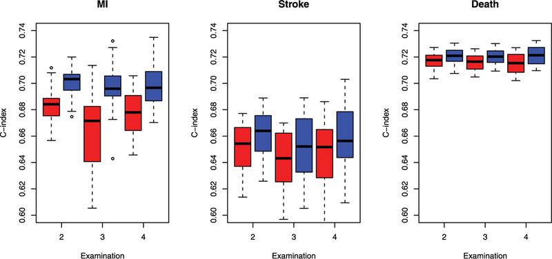
Boxplots of the estimates of the C-index at each examination in the ARIC study. The red boxes pertain to the univariate model of Fine and Gray (1999) for MI and stroke and the standard proportional hazards model for death. The blue boxes pertain to the proposed joint model.

We implicitly assume that K₁ and K₂ are greater than one; otherwise, some of the parameters need to be fixed to ensure identifiability. For example, if K₁ = K₂ = 1, we require ${\sigma }_2^2=0$ and γ₁ = 1; if K₁ > 1 and K₂ = 1, we require ${\sigma }_2^2=0$; and if K₁ = 1 and K₂ > 1, we require one of the γ_k’s to be 1. In the last scenario, we may set different γ_k to 1 and choose the model that yields the largest value of the likelihood function.

Remark 1.

The random effects b₁ and b₂ characterize the underlying health conditions for the asymptomatic and symptomatic events, respectively. The random effect for the asymptomatic events affects the kth symptomatic event through the unknown coefficient γ_k. For example, in the ARIC study, b₁ represents the common pathways for diabetes and hypertension, such as obesity, inflammation, oxidative stress, and insulin resistance, which also serve as potential risk factors for MI, stroke, and death. The random effect b₂ represents the underlying propensity for major cardiovascular diseases and death.

Suppose that the asymptomatic event time T_k (k = 1, …, K₁ ) is monitored at a sequence of positive time points $U_{k1}<\cdots <U_{k,M_k}$ and is known to lie in the interval (L_k, R_k], where L_k = max{U_kl : U_kl < T_k, l = 0, …, M_k}, and R_k = min{U_kl : U_kl ≥ T_k, l = 1, …, M_k + 1}, with U_k0 = 0 and $U_{k,M_k+1}=\infty$. Let C_k denote the censoring time on the symptomatic event time T_k (k = K₁ + 1, …, K) such that we observe Y_k = min(T_k, C_k) and Δ_k = I(T_k ≤ C_k), where I(·) is the indicator function. For a random sample of n subjects, the data consist of {O_i : i = 1, …, n}, where

$$\begin{array}{l}{\mathcal{O}}_i=\left\{L_{ik},R_{ik},{\mathit{X}}_{ik}(\cdot ):k=1,\dots ,K_1\right\}\cup \\ \hspace{1em}\hspace{1em}\times \left\{Y_{ik},{\Delta }_{ik},{\mathit{X}}_{ik}(\cdot ):k=K_1+1,\dots ,K\right\}.\end{array}$$

We assume that {U_ikl : k = 1, …, K₁; l = 1, …, M_ik} and {C_ik : k = K₁ + 1, …, K} are independent of {T_ik : k = 1, …, K} and b_i ≡ (b_i1, b_i2) conditional on {X_ik (·) : k = 1, …, K}. Then, the likelihood concerning the parameters θ ≡ (β, γ, Ʃ) and A ≡ (Λ₁, …, Λ_K) is

$$\begin{gathered} \prod _{i=1}^n{\int }_{b_i}\prod _{k=1}^{K_1}[\exp \left\{-{\int }_0^{L_{ik}}{e}^{{\mathit{\beta }}^{\text{T}}{\mathit{X}}_{ik}\left(s\right)+b_{i1}}d{\Lambda }_k\left(s\right)\right\} \\ \hspace{1em}\hspace{1em}-\exp \left\{-{\int }_0^{R_{ik}}{e}^{{\mathit{\beta }}^{\text{T}}{\mathit{X}}_{ik}\left(s\right)+b_{i1}}d{\Lambda }_k\left(s\right)\right\}] \\ \hspace{1em}\hspace{1em}\times \prod _{k=K_1+1}^K[{\left\{e^{{\mathit{\beta }}^{\text{T}}{\mathit{X}}_{ik}\left(Y_{ik}\right)+{\gamma }_k{b}_{i1}+b_{i2}}{\text{λ}}_k\left(Y_{ik}\right)\right\}}^{{\Delta }_{ik}} \\ \hspace{1em}\hspace{1em}\times \exp \left\{-{\int }_0^{Y_{ik}}{e}^{{\mathit{\beta }}^{\text{T}}{\mathit{X}}_{ik}\left(s\right)+{\gamma }_k{b}_{i1}+b_{i2}}d{\Lambda }_k\left(s\right)\right\}]\text{ψ}\left({\mathit{b}}_i;\mathit{\sum }\right)d{\mathit{b}}_i, \end{gathered}$$

where $\text{ψ}\left({\mathit{b}}_i;\sum \right)={\prod }_{j=1}^2\varphi \left(b_{ij};{\sigma }_j^2\right),$ $\varphi \left(b_{ij};{\sigma }_j^2\right)={\left(2\pi {\sigma }_j^2\right)}^{-1/2}\exp \left\{-b_{ij}^2/\left(2{\sigma }_j^2\right)\right\}$, ${\Lambda }_k\left(t\right)={\int }_0^t{\text{λ}}_{\text{k}}\left(s\right)ds$, and $\exp \left\{-{\int }_0^{\infty }{e}^{{\mathit{\beta }}^{\text{T}}{\mathit{X}}_{ik}\left(s\right)b_{i1}}d{\Lambda }_k\left(s\right)\right\}=0.$

In some studies, one of the symptomatic events is terminal (e.g., death), such that we have a semi-competing risks set-up (Fine, Jiang, and Chappell 2001), where the occurrence of the terminal event precludes the development of the other events but not vice versa. Without loss of generality, suppose that the Kth event is terminal. Then the monitoring times for T_k (k ≤ K₁) consist of the U_kl’s that are smaller than T_K , and the censoring time for T_k (k = K₁ + 1, …, K − 1) is min(C_k, T_K). Conditional on (b₁, b₂), the event times T₁, …, T_K−1 are mutually independent and are independent of the monitoring times and censoring times. Thus, for any set S_k that may depend on the monitoring times and censoring times, the joint probability of T₁ ∈ S₁, …, T_{K −1} ∈ S_K−1 conditional on (b₁, b₂ ) is equal to ${\prod }_{k+1}^{K-1}P\left(T_k\in S_k|b_1,b_2\right)$ with S_k as a deterministic set. Therefore, the likelihood remains the same as before.

2.2. Estimation Procedure

We adopt the nonparametric maximum likelihood estimation approach. For k = 1, …, K₁, let $0=t_{k0}<t_{k1}<t_{k2}<\cdots <t_{k,m_k}<\infty$ be the ordered sequence of all L_ik and R_ik with R_ik < ∞. For k = K₁ + 1, …, K, let $0=t_{k0}<t_{k1}<t_{k2}<\cdots <t_{k,m_k}<\infty$ be the ordered sequence of all Y_ik with Δ_ik = 1. The estimator for Λ_k (k = 1, …, K) is a step function that jumps only at $t_{k1},\dots ,t_{k,m_k}$ with respective jump sizes ${\text{λ}}_k\equiv \left({\text{λ}}_{k1},\dots ,{\text{λ}}_{k,m_k}\right)$. We maximize the objective function

$$\begin{array}{l}{L}_n\left(\text{θ},\mathcal{A}\right)=\prod _{i=1}^n{\int }_{{\mathit{b}}_i}\left\{\prod _{k=1}^{K_1}{g}_{ik}^{\left(1\right)}\left(b_{i1};\mathit{\beta },{\lambda }_k\right)\right\}\\ \hspace{1em}\hspace{1em}\hspace{1em}\hspace{1em}\hspace{1em}\times \left\{\prod _{k=K_1+1}^K{g}_{ik}^{\left(2\right)}\left({\mathit{b}}_i;\mathit{\beta },{\mathbf{\lambda }}_{\mathbf{k}}\right)\right\}\psi \left({\mathit{b}}_i;\sum \right)d{\mathit{b}}_i,\end{array}$$

over θ and λ₁, …., λ_K, where

$$\begin{array}{l}{g}_{iK}^{\left(1\right)}\left(b_{i1};\mathit{\beta },{\lambda }_k\right)=\exp \left(-\sum _{t_{Kl}\le L_{ik}}{e}^{{\mathit{\beta }}^{\text{T}}{\mathit{X}}_{ikl}+b_{i1}}{\text{λ}}_{Kl}\right)\\ \hspace{1em}\hspace{1em}\hspace{1em}\hspace{1em}\hspace{1em}\hspace{1em}\hspace{0.17em}\hspace{0.17em}-I\left(R_{ik}<\infty \right)\exp \left(-\sum _{t_{kl}\le R_{ik}}{e}^{{\mathit{\beta }}^{\text{T}}{\mathit{X}}_{ikl}+b_{i1}}{\text{λ}}_{kl}\right),\end{array}$$

$$\begin{array}{l}{g}_{iK}^{\left(2\right)}\left({\mathit{b}}_i;\mathit{\beta },{\lambda }_k\right)={\left[{\Lambda }_k\left\{Y_{ik}\right\}{e}^{{\mathit{\beta }}^{\text{T}}{\mathit{X}}_{ik}\left(Y_{ik}\right)+{\gamma }_k{b}_{i1}+b_{i2}}\right]}^{{\Delta }_{ik}}\\ \hspace{1em}\hspace{1em}\hspace{1em}\hspace{1em}\hspace{1em}\hspace{1em}\hspace{0.17em}\hspace{0.17em}\times \exp \left(-\sum _{t_{kl}\le Y_{ik}}{e}^{{\mathit{\beta }}^{\text{T}}{\mathit{X}}_{ikl}+b_{i1}+b_{i2}}{\text{λ}}_{kl}\right),\end{array}$$

X_ikl = X_ik (t_kl) for k = 1, …, K and l 1, …, m_k, and Λ_k{Y_ik} is the jump size of Λ_k at Y_ik.

Direct maximization of the objective function is difficult due to the lack of analytical expressions for λ₁, …, λ_K . We introduce latent Poisson random variables to form a likelihood equivalent to the objective function such that the maximum likelihood estimators can be easily obtained via a simple EM algorithm. For k = 1, …, K₁, we denote $R_{ik}^{*}=I\left(R_{ik}=\infty \right)L_{ik}+I\left(R_{ik}<\infty \right)R_{ik}$ and introduce independent Poisson random variables $W_{ikl}\left(l=1,\dots ,m_k,t_{kl}\le R_{ik}^{*}\right)$ with means λ_kl exp(β^TX_ikl + b_i1). Conditional on b_i1, the likelihood function of $\left\{W_{ikl};l=1,\dots ,m_k,t_{kl}\le R_{ik}^{*}\right\}$ is

$$\prod _{l=1,t_{kl}\le R_{ik}^{*}}^{m_k}\left\{\frac{1}{W_{ikl}!}{\left({\text{λ}}_{kl}{e}^{{\mathit{\beta }}^{\text{T}}{\mathit{X}}_{ikl}+b_{i1}}\right)}^{W_{ikl}}\exp \left(-{\text{λ}}_{kl}{e}^{{\mathit{\beta }}^{\text{T}}{\mathit{X}}_{ikl}+b_{i1}}\right)\right\}.$$

Let $A_{ik}={\sum }_{t_{kl}\le L_{ik}}{W}_{ikl}$ and $B_{ik}=I\left(R_{ik}<\infty \right){\sum }_{L_{ik}<t_{kl}\le R_{ik}}{W}_{ikl}$. The observed-data likehood for A_ik = 0 and B_ik > 0 given b_i1 is equal to

$$\begin{array}{l}\exp \left(-\sum _{t_{kl}\le L_{ik}}{e}^{{\mathit{\beta }}^{\text{T}}{\mathit{X}}_{ikl}+b_{i1}}{\text{λ}}_{kl}\right)\\ \hspace{1em}-I\left(R_{ik}<\infty \right)\exp \left(-\sum _{t_{kl}\le R_{ik}}{e}^{{\mathit{\beta }}^{\text{T}}{\mathit{X}}_{ikl}+b_{i1}}{\text{λ}}_{kl}\right),\end{array}$$

which is the same as $g_{ik}^{\left(1\right)}(b_{i1};\mathit{\beta },{\lambda }_k)$. Therefore, the objective function L_n(θ,A) can be viewed as the observed-data likelihood for {A_ik = 0, B_ik > 0 : i = 1, …, n; k = 1, …, K₁} ∪ {Y_ik,Δ_ik : i = 1, …, n; k = K₁ + 1, …, K} with $\left(W_{ikl},{\mathit{b}}_i\right)\left(i=1,\dots ,n;k=1,\dots ,K_1;l=1,\dots ,m_k,t_{kl}\le R_{ik}^{*}\right)$ as latent variables. In view of the foregoing results, we propose an EM algorithm treating W_ikl and b_i as missing data.

In the M-step, we maximize the conditional expectation of the complete-data log-likelihood given the observed data so as to update the parameters. In particular, the conditional expectation of the complete-data log-likelihood is

$$\begin{array}{l}\sum _{i=1}^n\widehat{E}(\sum _{k=1}^{K_1}[\sum _{l=1}^{m_k}I\left(t_{kl}\le R_{ik}^{*}\right)\{W_{ikl}\left(\log {\text{λ}}_{kl}+{\mathit{\beta }}^{\text{T}}{\mathit{X}}_{ikl}+b_{i1}\right)\\ \hspace{1em}-{\text{λ}}_{kl}\exp \left({\mathit{\beta }}^{\text{T}}{\mathit{X}}_{ikl}+b_{i1}\right)\}]\\ \hspace{1em}+\sum _{k=K_1+1}^K[{\Delta }_{ik}\left\{\log {\Lambda }_k\left\{Y_{ik}\right\}+{\mathit{\beta }}^{\text{T}}{\mathit{X}}_{ikl}\left(Y_{ik}\right)+{\gamma }_k{b}_{i1}+b_{i2}\right\}\\ \hspace{1em}-\sum _{t_{kl}\le Y_{ik}}{\text{λ}}_{kl}\exp \left({\mathit{\beta }}^{\text{T}}{\mathit{X}}_{ikl}+{\gamma }_k{b}_{i1}+b_{i2}\right)]),\end{array}$$ (3)

where $\widehat{E}(\cdot )$ denotes the conditional expectation given the observed data ${\tilde{\mathcal{O}}}_i\left(i=1,\dots ,n\right)$ , with ${\tilde{\mathcal{O}}}_i=\left\{A_{ik}=0,B_{ik}>0,{\mathit{X}}_{ik}(\cdot ):k=1,\dots ,K_1\right\}\cup \left\{Y_{ik},{\Delta }_{ik},{\mathit{X}}_{ik}(\cdot ):k=K_1+1,\dots ,K\right\}$. To update the parameters, we first differentiate (3) with respect to λ_kl (k = 1, …, K; l = 1, … ,m_k) to obtain the updating formulas for λ_k:

$${\text{λ}}_{kl}=\frac{{\sum }_{i=1}^{n}I\left(t_{kl}\le R_{ik}^{*}\right)\widehat{E}\left(W_{ikl}\right)}{{\sum }_{i=1}^{n}I\left(t_{kl}\le R_{ik}^{*}\right)\widehat{E}\left\{\exp \left({\mathit{\beta }}^{\text{T}}{\mathit{X}}_{ikl}+b_{i1}\right)\right\}}$$ (4)

for k = 1,…, K and l = 1 , …, m_k and

$${\text{λ}}_{kl}=\frac{{\sum }_{i=1}^n{\Delta }_{ik}I\left(Y_{ik}=t_{kl}\right)}{{\sum }_{i=1}^{n}I\left(Y_{kl}\ge t_{kl}\right)\widehat{E}\left\{\exp \left({\mathit{\beta }}^{\text{T}}{\mathit{X}}_{ikl}+{\gamma }_k{b}_{i1}+b_{i2}\right)\right\}}$$ (5)

for k = K₁+1; l = K and l = 1, …, m_k). We then update β by solving the equation.

$$\begin{gathered} \sum _{i=1}^n\{\sum _{k=1}^{K_1}\sum _{l=1}^{m_k}\widehat{E}\left(W_{ikl}\right)I\left(t_{kl}\le R_{ik}^{*}\right)\left[{\mathit{X}}_{ikl}-\frac{{\sum }_{j=1}^n{\mathit{X}}_{jkl}I\left(t_{kl}\le R_{jk}^{*}\right)\widehat{E}\left\{\exp \left({\mathit{\beta }}^{\text{T}}{\mathit{X}}_{jkl}+b_{j1}\right)\right\}}{{\sum }_{j=1}^{n}I\left(t_{kl}\le R_{jk}^{*}\right)\widehat{E}\left\{\exp \left({\mathit{\beta }}^{\text{T}}{\mathit{X}}_{jkl}+b_{j1}\right)\right\}}\right] \\ \hspace{1em}+\sum _{k=K_1=1}^K{\Delta }_{ik}\left({\mathit{X}}_{ik}\left(Y_{ik}\right)-\frac{{\sum }_{j=1}^{n}I\left(Y_{jk}\ge Y_{ik}\right){\mathit{X}}_{jk}\left(Y_{ik}\right)\widehat{E}\left[\exp \left\{{\mathit{\beta }}^{\text{T}}{\mathit{X}}_{jk}\left(Y_{ik}\right)+{\gamma }_k{b}_{j1}+b_{j2}\right\}\right]}{{\sum }_{j=1}^{n}I\left(Y_{jk}\ge Y_{ik}\right)\widehat{E}\left[\exp \left\{{\mathit{\beta }}^{\text{T}}{\mathit{X}}_{jk}\left(Y_{ik}\right)+{\gamma }_k{b}_{j1}+b_{j2}\right\}\right]}\right)\}=0 \end{gathered}$$

and update γ_k by solving the equation

$$\sum _{i=1}^n{\Delta }_{ik}\left(\widehat{E}\left(b_{i1}\right)-\frac{{\sum }_{j=1}^{n}I\left(Y_{jk}\ge Y_{ik}\right)\widehat{E}\left[b_{j1}\exp \left\{{\mathit{\beta }}^{\text{T}}{\mathit{X}}_{jk}\left(Y_{ik}\right)+{\gamma }_k{b}_{j1}+b_{j2}\right\}\right]}{{\sum }_{j=1}^{n}I\left(Y_{jk}\ge Y_{ik}\right)\widehat{E}\left[\exp \left\{{\mathit{\beta }}^{\text{T}}{\mathit{X}}_{jk}\left(Y_{ik}\right)+{\gamma }_k{b}_{j1}+b_{j2}\right\}\right]}\right)=0.$$

The two equations are obtained by differentiating (3) with respect to β_k or γ_k and replacing λ_kl by the right hand side of (4) or (5). Finally, we update ${\sigma }_j^2$ by ${\sigma }_j^2={\sum }_{i=1}^n\widehat{E}\left(b_{ij}^2\right)/n$ for j = 1, 2.

In the E-step, we evaluate the conditional expectation of $W_{ikl}\left(k=1,\dots ,K_1;l=1,\dots ,m_k,t_{kl}\le R_{ik}^{*}\right)$ and the other terms of b_i given the observed data ${\tilde{\mathcal{O}}}_i$ for i = 1, …, n. Specifically, the conditional expectation of $W_{ikl}\left(k=1,\dots ,K_1;l=1,\dots ,m_k,t_{kl}\le R_{ik}^{*}\right)$ given ${\tilde{\mathcal{O}}}_i$ and b_i is

$$I\left(L_{ik}<t_{kl}\le R_{ik}<\infty \right)\frac{{\lambda }_{kl}\exp \left({\mathit{\beta }}^{\text{T}}{\mathit{X}}_{ikl}+b_{i1}\right)}{1-\exp \left(-{\sum }_{L_{ik}<t_{k{l}^{\prime }}\le R_{ik}}{\text{λ}}_{k{l}^{\prime }}{e}^{{\mathit{\beta }}^{\text{T}}{\mathit{X}}_{ik{l}^{\prime }}+b_{i1}}\right)}.$$

Note that the density of b_i given ${\tilde{\mathcal{O}}}_i$ is proportional to $\left\{{\prod }_{k=1}^{K_1}{g}_{ik}^{\left(1\right)}\left(b_{i1};\mathit{\beta },{\text{λ}}_k\right)\right\}\times \left\{{\prod }_{k=K_1+1}^{K_1}{g}_{ik}^{\left(1\right)}\left({\mathit{b}}_i;\mathit{\beta },{\lambda }_k\right)\right\}\psi \left({\mathit{b}}_i;\sum \right)$. We evaluate the conditional expectation of W_ikl and the other terms through numerical integration over b_i with Gauss–Hermite quadratures.

We iterate between the E-step and M-step until convergence. In the M-step, the high-dimensional nuisance parameters λ_kl (k = 1, …, K; l = 1, …, m_k) are calculated explicitly, such that inversion of high-dimensional matrices is avoided. We denote the final estimators for θ and A as $\widehat{\theta }\equiv \left(\widehat{\beta },\widehat{\gamma },\widehat{\sum }\right)$ and $\widehat{\mathcal{A}}\equiv \left({\widehat{\Lambda }}_1,\dots ,{\widehat{\Lambda }}_K\right)$.

2.3. Asymptotic Theory

We establish the asymptotic properties of $\left(\widehat{\theta },\widehat{{\rm A}}\right)$ under the following regularity conditions.

Condition 1.

The true value of θ, denoted by θ₀ ≡ (β₀, γ₀, Ʃ₀), belongs to the interior of a known compact set $\Theta \equiv B\times \mathcal{G}\times \mathcal{S}$ , where $B\subset {ℝ}^p,\mathcal{G}\subset {ℝ}^{K_2}$ , and S ⊂ (0, ∞) × (0, ∞).

Condition 2.

For k = 1, …, K, the true value Λ_k0 (·) of Λ_k (·) is strictly increasing and continuously differentiable in [0, τ_k] with Λ_k0 (0) = 0.

Condition 3.

For k = 1, …, K₁, the monitoring times have finite support U_k with the least upper bound τ_k. The number of potential monitoring times M_k is positive with E(M_k) < ∞. There exists a positive constant η such that $\mathrm{Pr}\left\{{\min }_{1\le k\le K_1,0\le m<M_k}\left(U_{k,m+1}-U_{km}\right)\ge \eta |M_k,{{\rm X}}_k\right\}=1$. In addition, there exists a probability measure μ_k in U_k such that the bivariate distribution function of (U_km, U_k,m+1) conditional on (M_k, X_k) is dominated by μ_k × μ_k and its Radon–Nikodym derivative, denoted by ${\tilde{f}}_{km}\left(u,\upsilon ;M_k,{{\rm X}}_k\right)$ , can be expanded to a positive and twice-continuously differentiable function in the $set\left\{\left(u,\upsilon \right):0\le u\le {\tau }_k,0\le \upsilon \le {\tau }_k,\upsilon -u\ge \eta \right\}$.

Condition 4.

For k = K₁ + 1, …, K, let τ_k denote the study duration time and U_k = [0, τ_k]. There exists a positive constant δ such that $\text{pr}\left(C_k\ge {\tau }_k|{{\rm X}}_k\right)=\text{pr}\left(C_k={\tau }_k|{{\rm X}}_k\right)\ge \delta$ almost surely.

Condition 5.

With probability 1, X_k (·) has bounded total variation in U_k. If there exists a constant vector a₁ and a deterministic function a_2k (t) such that ${\text{a}}_1^T{{\rm X}}_k\left(t\right)+a_{2k}\left(t\right)=0$ for any t ∈ U_k and any k ∈ {1, …, K} with probability 1, then a₁ = 0 and a_2k (t) = 0 for any t ∈ U_k and any k ∈ {1, …, K}.

Remark 2.

Conditions 1, 2, and 5 are standard conditions for failure time regression with time-dependent covariates. Condition 3 pertains to the joint distribution of monitoring times of the asymptomatic events. It requires that two adjacent monitoring times are separated by at least η; otherwise, the data may contain exact observations, which require a different theoretical treatment. The dominating measure μ_k is chosen as the Lebesgue measure if the monitoring times are continuous random variables and as the counting measure if monitorings occur only at a finite number of time points. The number of potential monitoring times M_k can be fixed or random, is possibly different among study subjects and event types, and is allowed to depend on covariates. Condition 4 implies that there is a positive probability for the kth symptomatic event to be observed in the time interval [0, τ_k].

We state the strong consistency of $\left(\widehat{\theta },\widehat{{\rm A}}\right)$ and the weak convergence of $\widehat{\theta }$ in two theorems.

Theorem 1.

Under Conditions 1−5, $\Vert \widehat{\theta }-{\theta }_0\Vert {\to }_{a.s.}0$, and ${\Vert {\widehat{\Lambda }}_k-{\Lambda }_{k0}\Vert }_{l^{\infty }\left({\mathcal{U}}_k\right)}{\to }_{a.s.}0$, where ${\Vert \cdot \Vert }_{l^{\infty }\left({\mathcal{U}}_k\right)}$ denotes the supremum norm on U_k for k = 1,…,K.

Theorem 2.

Under Conditions 1−5, $n^{1/2}\left(\widehat{\theta },{\theta }_0\right)$ converges weakly to a ( p + K₂ + 2)-dimensional zero-mean normal random vector with a covariance matrix that attains the semiparametric efficiency bound.

The proofs of all theorems are provided in the Section S.1 of the supplementary materials.

We propose two approaches to estimate the covariance matrix of $\widehat{\mathit{\theta }}$. The first approach makes use of the profile likelihood (Murphy and Van der Vaart 2000). Specifically, we define the profile log-likelihood function

$$p{l}_n\left(\mathit{\theta }\right)=\underset{\mathcal{A}\in {\mathcal{C}}_1\times \cdots \times {\mathcal{C}}_k}{\max }\log L_n\left(\mathit{\theta }\text{,}\mathcal{A}\right),$$

where C_k is the set of step functions with nonnegative jumps at t_kl (k = 1, …, K; l = 1, …, m_k). We estimate the covariance matrix of $\widehat{\mathit{\theta }}$ by the inverse of

$${\sum _{i=1}^n\left(\begin{array}{c}\frac{p{l}_i\left(\widehat{\mathit{\theta }}+h_n{e}_1\right)-p{l}_i\left(\widehat{\mathit{\theta }}\right)}{h_n}\\ ⋮\\ \frac{p{l}_i\left(\widehat{\mathit{\theta }}+h_n{e}_{p+k_2+2}\right)-p{l}_i\left(\widehat{\mathit{\theta }}\right)}{h_n}\end{array}\right)}^{\otimes 2},$$

where pl_i is the ith subject’s contribution to pl_n, e_j is the jth canonical vector in ${ℝ}^{p+k_2+2}$ , a^⊗2 = aa^T, and h_n is a constant of order n^−1/2. To evaluate the profile likelihood, we use the EM algorithm of Section 2.2 but only update Λ₁, …, Λ_K in the M-step.

Alternatively, we approximate the asymptotic distribution of $\widehat{\mathit{\theta }}$ by bootstrapping the observations. In particular, we draw a simple random sample of size n with replacement from the observed data {O_i : i = 1, …, n}. Let ${\widehat{\mathit{\theta }}}^{\ast }$ be the estimator of θ bootstrap sample. The empirical distribution ${\widehat{\mathit{\theta }}}^{\ast }$ in the bootstrap sample. The empirical distribution of ${\widehat{\mathit{\theta }}}^{\ast }$ can be used to approximate the distribution of $\widehat{\mathit{\theta }}$ Confidence intervals for θ₀ can be constructed by the Wald method (with the variance of ${\widehat{\mathit{\theta }}}^{\ast }$ ) or from the empirical percentiles of ${\widehat{\mathit{\theta }}}^{\ast }$. The following theorem states the asymptotic properties of ${\widehat{\mathit{\theta }}}^{\ast }$ thereby validating the bootstrap procedure.

Theorem 3.

Under Conditions 1−5, the conditional distribution of $n^{1/2}\left({\widehat{\mathit{\theta }}}^{\ast }-\widehat{\mathit{\theta }}\right)$ given the data converges weakly to the asymptotic distribution of $n^{1/2}\left({\widehat{\mathit{\theta }}}^{\ast }-\widehat{\mathit{\theta }}\right)$.

2.4. Dynamic Prediction

Given the fitted joint model, we can predict future events by updating the event history. For a subject with covariates X, let O(t ) denote the event history at time t > 0, which includes the interval-censored observations of the asymptomatic events {L_k(t ), R_k(t) : k = 1, …, K₁}, and the right-censored observations of the symptomatic events {Y_k(t ),Δ_k(t) : k = K₁ + 1, …, K}.

If no event history is available, the density of the random effect b can be estimated by $\psi \left(\mathit{b};\widehat{\mathit{\sum }}\right)$ . We estimate the survival function of T_k, denoted by P(T_k ≥ t|X), by

$${\int }_{\mathit{b}}{s}_k\left(t;\mathit{{\rm X}};\hspace{0.17em}\mathit{b}\right)\psi \left(\mathit{b};\widehat{\mathit{\sum }}\right)d\mathit{b},$$

where

$$s_k\hspace{0.17em}\mathit{X},\hspace{0.17em}b)$$

$$=\{\begin{array}{l}\exp \left\{-{\int }_0^t{e}^{{\widehat{\beta }}^{\text{T}}{\mathit{X}}_k\left(u\right)+b_1}d{\widehat{\Lambda }}_k\left(u\right)\right\}\hspace{1em}\hspace{1em}\hspace{0.17em}\hspace{0.17em}k=1,\dots ,K_1\\ \exp \left\{-{\int }_0^t{e}^{{\widehat{\beta }}^{\text{T}}{X}_k\left(u\right)+{\widehat{\gamma }}_k{b}_1+b_2}d{\widehat{\Lambda }}_k\left(u\right)\right\}\hspace{1em}\hspace{0.17em}k=K_1+1,\dots ,K\end{array},$$

and the integral is evaluated by numerical integration with Gauss–Hermite quadratures. Here, the function sk(t; X, b) can be interpreted as the conditional survival probability of T_k at time t given b and X.

In the semi-competing risks set-up, where one of the symptomatic events is terminal, it is more meaningful to use the cumulative incidence function to predict the event time of interest. Without loss of generality, we assume the Kth event is terminal. The cumulative incidence function of the kth event

(k = 1, …, K − 1) is given by

$$P\left(T_k\le t,T_k\le T_K|\mathit{{\rm X}}\right)\hspace{1em}={\int }_{\mathit{b}}\left\{P\left(T_k\le t\le T_k|\mathit{{\rm X}}\text{,}\mathit{b}\right)+P\left(T_k\le T_K<t|\mathit{{\rm X}},\mathit{b}\right)\right\}\psi \left(\mathit{b};\sum \right)d\mathit{b}\hspace{1em}={\int }_{\mathit{b}}\{P\left(T_k\le t|T_k\ge t,\mathit{{\rm X}}\text{,}\mathit{b}\right)P\left(T_K\ge t|\mathit{{\rm X}}\text{,}\mathit{b}\right)\hspace{1em}\hspace{1em}+{\int }_0^{t}P\left(T_k\le u|T_K=u,\mathit{{\rm X}}\text{,}\mathit{b}\right)dP\left(T_K\le u|\mathit{{\rm X}}\text{,}\mathit{b}\right)\}\psi \left(\mathit{b};\sum \right)d\mathit{b},$$

which can be estimated by

$$\begin{array}{l}{\int }_{\text{b}}\left[\left\{1-s_k\left(t;{\rm X},b\right)\right\}{s}_k\left(t;X,b\right)\right.\\ +{\int }_0^t\left.\left\{1-s_k\left(u;{\rm X},b\right)\right\}{s}_k\left(u;X,b\right)e^{{\widehat{\beta }}^{\text{T}}{\text{X}}_K\left(u\right)+{\widehat{\gamma }}_K{b}_1+b_2}d{\widehat{\Lambda }}_K\left(u\right)\right]\\ \times \psi \left(b;\widehat{\sum }\right)db\text{.}\end{array}$$

Here, the function sk(t; X, b) can be interpreted as the conditional survival probability of Tk at time t given T_K ≥ t, b, and X.

At time t₀ > 0, we update the posterior density of b given the event history O(t₀) so as to perform dynamic prediction. Note that the posterior density of b is proportional to

$$\begin{array}{l}J\left(\mathit{b};t_0,\mathit{X}\right)\equiv \prod _{k=1}^{K_1}\left\{s_k\left(L_k\left(t_0\right);\mathit{X},\mathit{b}\right)-s_k\left(R_k\left(t_0\right);\mathit{X},\mathit{b}\right)\right\}\\ \hspace{1em}\hspace{1em}\hspace{1em}\hspace{1em}\hspace{1em}\times \prod _{k=K_1+1}^K(s_k\left(Y_k\left(t_0\right);\mathit{X},\mathit{b}\right)\\ \hspace{1em}\hspace{1em}\hspace{1em}\hspace{1em}\hspace{1em}\times {\left[{\widehat{\Lambda }}_k\left\{Y_k\left(t_0\right)\right\}{e}^{{\widehat{\beta }}^{\text{T}}{\mathit{X}}_k\left\{Y_k\left(t_0\right)\right\}+{\widehat{\gamma }}_k{b}_1+b_2}\right]}^{{\Delta }_k\left(t_0\right)})\psi \left(\mathit{b};\widehat{\sum }\right).\end{array}$$

If the subject has not developed the kth event or the terminal event by time t₀, that is, Y_k(t₀) = Y_K (t₀) = t₀ and Δ_k(t₀) =Δ_K (t0) = 0, we estimate the conditional cumulative incidence function of the kth event, P(T_k ≤ t, T_k ≤ T_K|O(t₀ ), X), by

$$\begin{array}{l}{\int }_{\mathit{b}}\frac{j\left(\mathit{b};t_0,\mathit{X}\right)}{s_k\left(t_0;\mathit{X},\mathit{b}\right)s_K\left(t_0;\mathit{X},\mathit{b}\right){\int }_{{\mathit{b}}^{\prime }}j\left({\mathit{b}}^{\prime };t_0,\mathit{X}\right)d{\mathit{b}}^{\prime }}\\ \hspace{1em}\times [\left\{s_k\left(t_0;\mathit{X},\mathit{b}\right)-s_k\left(t;\mathit{X},\mathit{b}\right)\right\}{s}_K\left(t;\mathit{X},\mathit{b}\right)\\ \hspace{1em}+{\int }_{t_0}^t\left\{s_k\left(t_0;\mathit{X},\mathit{b}\right)-s_k\left(u;\mathit{X},\mathit{b}\right)\right\}\\ \hspace{1em}\times s_K\left(u;\mathit{X},\mathit{b}\right)e^{{\widehat{\beta }}^{\text{T}}{\mathit{X}}_K\left(u\right)+{\widehat{\gamma }}_K{b}_1+b_2}d{\widehat{\Lambda }}_K\left(u\right)]d\mathit{b}.\end{array}$$

In practice, it is desirable to identify subjects who are at increased risk as the event history is accumulating. In the same vein as the risk score under the standard proportional hazards model, we use the risk score ${\widehat{\beta }}^{\text{T}}{{\rm X}}_k\left(t_0\right)+{\widehat{\gamma }}_k{\widehat{\mathit{b}}}_1\left(t_0\right)+{\widehat{\mathit{b}}}_2\left(t_0\right)$ to dynamically predict the kth event (k = K₁ + 1, …, K), where $\widehat{\mathit{b}}\left(t_0\right)\equiv \left({\widehat{\mathit{b}}}_1\left(t_0\right)+{\widehat{\mathit{b}}}_2\left(t_0\right)\right)$ is a suitable estimator of b given the event history O(t₀). The estimator $\widehat{\mathit{b}}\left(t_0\right)$ can be the posterior mean or mode of b or an imputed value from the posterior distribution. For example, the risk score using the posterior mean is given by

$${\widehat{\beta }}^{\text{T}}{\mathit{X}}_k\left(t_0\right)+\frac{{\int }_{\mathit{b}}\left({\widehat{\gamma }}_k{b}_1+b_2\right)J\left(\mathit{b};t_0,\mathit{X}\right)d\mathit{b}}{{\int }_{\mathit{b}}J\left(\mathit{b};t_0,\mathit{X}\right)d\mathit{b}}.$$

The risk score quantifies the subject-specific risk and can be very useful to both individual patients and clinicians when making decisions about lifestyle modifications and preventive medical treatments.

3. Simulation Studies

We conducted simulation studies to assess the performance of the proposed methods. We considered one time-independent covariate X₁ ∼ Unif(0, 1) and one time-dependent covariate X₂(t) = I(t ≤ V)B₁ + I(t > V)B₂, where B₁ and B₂ are independent Bernoulli(0.5), V ∼ Unif(0, τ), and τ = 4. We considered two asymptomatic events and two symptomatic events. We set X_k = e_k ⊗ (X₁, X₂)^T, where e_k is the kth canonical vector in ${ℝ}^4$, and ⊗ denotes the Kronecker product. We set β = (0.5, 0.4, 0.5,−0.2,−0.5, 0.5,−0.5, 0.5)^T, Λ₁(t) = 0.5t, Λ_k(t) = log{1 + t/(k − 1)} for k = 2, 3, 4, γ₃ = γ₄ = 0.25, and σ₂¹ = σ₂² = 1. Both symptomatic events were censored by C ∼ Unif(2τ/3, τ), such that the censoring rates are 33% and 39%, respectively. The series of monitoring times were generated sequentially, with U_m = U_m−1 + 0.1 + Unif (0, 0.5) for m ≥ 1 and U₀ = 0. The last monitoring time is the largest U_m that is smaller than C. We set n = 100 or 200 and simulated 2000 replicates. For each dataset, we applied the proposed EM algorithm by setting the initial value of β to 0, the initial values of γ_k and σ_k² to 1 and the initial value of λ_kl to 1/m_k. We used 20 quadrature points for integration with respect to each random effect and set the convergence threshold to 10⁻³. For variance estimation, we set h_n = 5n^−1/2 for profile likelihood and used 100 bootstrap samples.

Table 1 summarizes the simulation results. The biases for all parameter estimators are small, especially for n = 200. Both the profile-likelihood and bootstrap variance estimators for $\widehat{\beta }$ are accurate, especially for n = 200. Both variance estimators for $\widehat{\gamma }$ tend to overestimate the true variabilities, but the coverage probabilities of the confidence intervals get closer to the nominal level as sample size increases. The profile-likelihood variance estimators for ${\widehat{\sigma }}_1^2$ and ${\widehat{\sigma }}_2^2$ overestimate the true variabilities, while the bootstrap variance estimators for ${\widehat{\sigma }}_1^2$ and ${\widehat{\sigma }}_2^2$ accurately reflect the true variabilities. Figure S.1(a) of the Supplemental Materials shows the estimation of the baseline survival functions with sample size n = 200. The estimators are virtually unbiased.

Table 1.

Summary statistics for the simulation studies without a terminal event.

	n = 100						n = 200
			Profile		Bootstrap				Profile		Bootstrap
	Bias	SE	SEE	CP	SEE	CP	Bias	SE	SEE	CP	SEE	CP
β11	0.006	0.585	0.597	0.961	0.627	0.967	0.027	0.405	0.399	0.947	0.412	0.953
β12	0.029	0.327	0.321	0.941	0.348	0.960	0.019	0.222	0.216	0.949	0.228	0.953
β21	0.015	0.623	0.609	0.946	0.648	0.963	0.014	0.410	0.409	0.951	0.424	0.958
β22	−0.005	0.341	0.329	0.940	0.355	0.962	−0.002	0.225	0.222	0.9(51	0.233	0.961
β31	−0.022	0.617	0.635	0.957	0.610	0.949	−0.004	0.416	0.428	0.960	0.420	0.948
β32	−0.002	0.319	0.338	0.965	0.322	0.949	0.009	0.221	0.229	0.958	0.222	0.947
β41	−0.012	0.623	0.651	0.969	0.629	0.955	0.006	0.449	0.440	0.947	0.431	0.942
β42	0.004	0.330	0.348	0.967	0.332	0.950	−0.001	0.231	0.235	0.955	0.229	0.945
γ3	−0.012	0.227	0.252	0.979	0.260	0.971	−0.012	0.159	0.171	0.962	0.170	0.960
γ3	−0.013	0.237	0.260	0.976	0.266	0.972	−0.016	0.162	0.173	0.966	0.177	0.963
${\sigma }_1^2$	0.062	0.445	0.751	0.978	0.493	0.956	0.031	0.317	0.482	0.982	0.318	0.946
${\sigma }_2^2$	−0.102	0.413	0.510	0.993	0.482	0.971	−0.062	0.297	0.335	0.987	0.312	0.974

NOTE: SE and SEE denote, respectively, the empirical standard error and mean standard error estimator. CP stands for the empirical coverage probability of the % confidence interval based on the Wald method for the profile-likelihood approach and the % symmetric confidence interval for the bootstrap approach. For γ₃, γ₄, ${\sigma }_1^2$, and ${\sigma }_2^2$, bias and SEE are based on the median instead of the mean, and SE is based on the mean absolute deviation. For ${\sigma }_1^2$ and ${\sigma }_2^2$, the confidence intervals are based on the log transformation.

We considered a second setup with an additional terminal event. We set X_k = e_k ⊗ (X₁, X₂)^T, where e_k is the kth canonical vector in ${ℝ}^5$. In addition, we set β = (0.5, 0.4, 0.5, −0.2, −0.5, 0.5, −0.5, 0.5, 0.3, −0.2)^T, Λ₅ (t) = log(1 + t/4), and γ₅ = 0.25. The terminal event was also censored by C. The censoring rates for the right-censored events are 51%, 58%, and 43%, respectively. The results are shown in Table S.1 and Figure S.1(b) of the supplemental materials. The conclusions are similar to the case of no terminal event.

We assessed the performance of dynamic prediction based on the conditional cumulative incidence function in the setting with a terminal event. Suppose that at the first monitoring time t₀ = 1, event 2 has occurred but events 1, 3, and 4 have not. Figure 1 shows the estimation of the baseline cumulative incidence functions (pertaining to X = 0) for events 3 and 4 given the event history at time t₀ = 1. The estimators slightly underestimate the true values at the right tail, but the biases get smaller as n increases.

Figure 1.

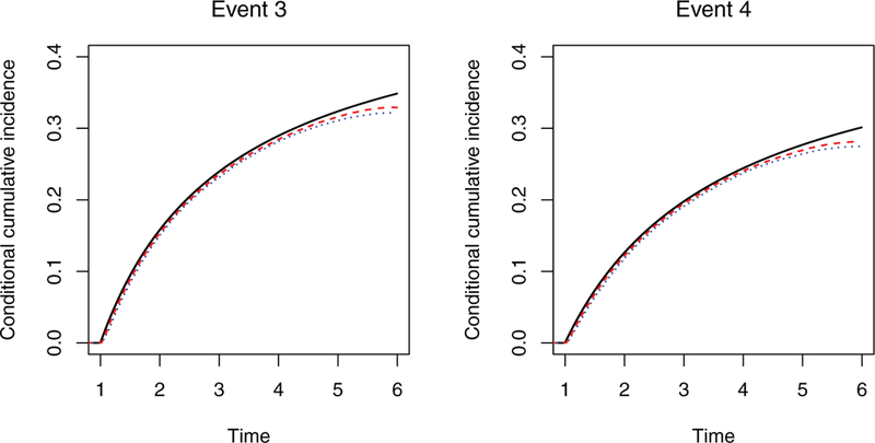
Estimation of the baseline cumulative incidence function conditional on the event history. The solid black curve, dotted blue curve, and dashed red curve pertain, respectively, to the true value and the mean estimates from the proposed method with n = 100 and n = 200.

To investigate the performance of the proposed dynamic prediction methods under misspecified models, we conducted another set of simulation studies where the event times were generated from the proportional odds, instead of the proportional hazards, models with random effects. As shown in Section S.2 of the supplemental materials, the dynamic prediction is still quite accurate.

4. ARIC Study

ARIC is a perspective epidemiological cohort study conducted in four U.S. communities: Forsyth County, NC; Jackson, MS; Minneapolis, MN; and Washington County, MD. A total of 15792 participants received a baseline examination between 1987 and 1989 and four subsequent examinations in 1990–1992, 1993–1995, 1996–1998, and 2011–2013. At each examination, medical data were collected, such that interval-censored observations for diabetes and hypertension were obtained. The participants were also followed for cardiovascular diseases through reviews of hospital records, such that potentially right-censored observations on MI, stroke, and death were collected.

We related the disease incidence to race, sex, and five baseline risk factors: age, body mass index (BMI), glucose level, systolic blood pressure, and smoking status. Since the Jackson cohort is composed of black subjects only, and neither Minneapolis nor Washington County cohorts contain black subjects, we included the cohort×race indicators as predictors. We excluded subjects with prevalent cases at baseline or missing covariate values to obtain a total of 8728 subjects. During the study, 17.3%, 46.8%, 8.3%, and 5.1% of the subjects developed diabetes, hypertension, MI, and stroke, respectively, while 28.7% died.

We jointly modeled the asymptomatic and symptomatic events in the ARIC study with equations (1) and (2). For variance estimation, we used the profile likelihood approach with h_n = 5n^−1/2. Tables 2 and 3 show the estimation results for the regression parameters. Several characteristics and baseline risk factors are found to be predictive of the events. Older subjects have higher risks of hypertension, MI, stroke, and death than younger subjects. Males have lower risk of hypertension but higher risks of MI, stroke, and death than females. Smokers have significantly higher risks for all events than non-smokers. In addition, higher baseline BMI increases the risks of diabetes, hypertension, and MI; higher baseline glucose level increases the risks of diabetes, stroke, and death; and higher baseline value of systolic blood pressure increases the risks of all considered events.

Table 2.

Estimation results for the regression parameters of the asymptomatic events in the ARIC study.

	Diabetes			Hypertension
Covariate	Estimate	Std error	p-value	Estimate	Std error	p-value
Forsyth County, white	−0.5332	0.1817	0.0033	−0.5032	0.0615	<0.0001
Jackson, black	−0.1356	0.1806	0.4530	−0.1075	0.0673	0.1104
Minneapolis, white	−0.9415	0.1802	<0.0001	−0.5747	0.0579	<0.0001
Washington County, white	−0.3778	0.1778	0.0336	−0.3798	0.0592	<0.0001
Age	−0.0093	0.0057	0.1025	0.0166	0.0036	<0.0001
Male	−0.0655	0.0593	0.2694	−0.2329	0.0396	<0.0001
BMI	0.0911	0.0059	<0.0001	0.0254	0.0044	<0.0001
Glucose	0.1075	0.0033	<0.0001	0.0004	0.0023	0.8744
Systolic blood pressure	0.0096	0.0026	0.0003	0.0780	0.0022	<0.0001
Smoker	0.4576	0.0674	<0.0001	0.3134	0.0468	<0.0001

NOTE: The blacks in Forsyth County form the reference group for the cohort×race variables.

Table 3.

Estimation results for the regression parameters of the symptomatic events in the ARIC study.

	Ml			Stroke			Death
Covariate	Estimate	Std error	p-value	Estimate	Std error	p-value	Estimate	Std error	p-value
Forsyth County, white	0.0467	0.2477	0.8504	0.1308	0.3688	0.7228	−0.2475	0.1049	0.0183
Jackson, black	−0.3121	0.2681	0.2444	0.6622	0.3755	0.0778	0.1871	0.1118	0.0941
Minneapolis, white	−0.1052	0.2476	0.6710	0.0507	0.3688	0.8907	−0.3262	0.1040	0.0017
Washington County, white	0.1953	0.2457	0.4266	0.5013	0.3653	0.1700	−0.1194	0.1032	0.2471
Age	0.0805	0.0078	<0.0001	0.1121	0.0099	<0.0001	0.1465	0.0054	<0.0001
Male	0.9279	0.0901	<0.0001	0.4050	0.1071	0.0002	0.6108	0.0545	<0.0001
BMI	0.0273	0.0101	0.0068	−0.0010	0.0123	0.9356	0.0080	0.0060	0.1847
Glucose	0.0059	0.0046	0.2007	0.0215	0.0057	0.0002	0.0104	0.0030	0.0006
Systolic blood pressure	0.0135	0.0036	0.0002	0.0192	0.0047	<0.0001	0.0089	0.0022	0.0001
Smoker	1.2378	0.0888	<0.0001	1.0023	0.1127	<0.0001	1.3045	0.0599	<0.0001

NOTE: See the Note to Table 2

The estimation results for the remaining parametric components are shown in Table S.2 of the supplemental materials. The variance components σ₁² and σ₂² are significantly larger than zero, indicating strong correlation among the asymptomatic events and among the symptomatic events. The parameters γ_MI, γ _Stroke, and γ_Death are also significantly larger than zero, reflecting the strong positive dependence of the symptomatic events on the asymptomatic events. The Akaike information criterion (AIC) for the proposed model is 108852.8. For comparisons, we also fit a model with one random effect shared by all events. The corresponding AIC is 109000.6, and the p-value for the likelihood ratio test is less than 0.0001, indicating that the proposed model provides a much better fit to the data than the model with one shared random effect.

To evaluate the performance of the proposed prediction methods, we randomly divided the study cohort into training and testing sets with equal numbers of subjects. We analyzed the training set to obtain parameter estimates, based on which we calculated the risk scores for subjects in the testing set, where the posterior means of the random effects were used. Specifically, at examinations 2, 3, and 4, we calculated the risk scores of MI or stroke for subjects who have not developed the disease. We evaluated the performance of the prediction using C-index (Uno et al. 2011) and compared it with that of the risk scores based on the standard models. In particular, for MI and stroke, we considered the univariate model of Fine and Gray (1999) with death as a competing risk; for death, we considered the standard proportional hazards model. The values of the C-index based on twenty randomly divided training/test tests are shown in Figure 2. The proposed risk score performs better than the risk score of the standard model at all examinations for all symptomatic events.

Figure 3 shows the estimated conditional cumulative incidence functions of MI and stroke for two smokers and two non-smokers who have different event histories at year 3 but with the same values of other risk factors. The risks of MI and stroke are considerably higher for the smokers than the non-smokers with the same event history. The estimated conditional probabilities for the subjects who have developed both diabetes and hypertension are higher than those who have not developed diabetes or hypertension.

Figure 3.

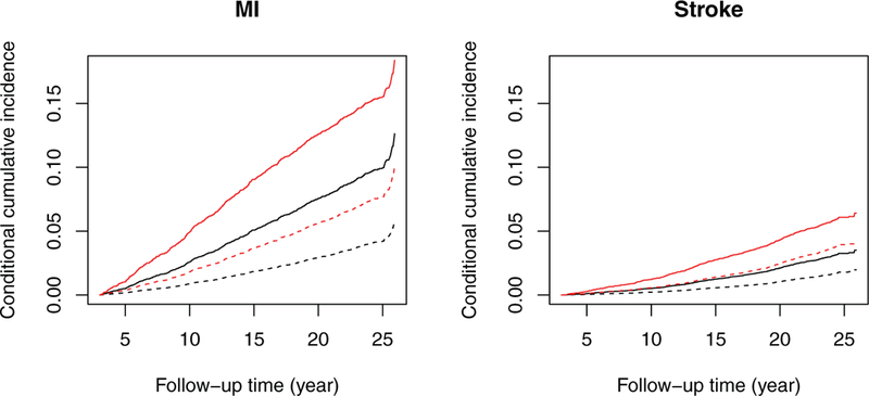
Estimation of the conditional cumulative incidence functions of MI and stroke for a 50-year-old white female residing in Forsyth County, NC, with BMI 40 kg/m², glucose 98 mg/dL, and systolic blood pressure mmHg. The solid curves pertain to smokers, while the dashed curves pertain to non-smokers. The black curves pertain to subjects who have not developed diabetes or hypertension by year 3. The red curves pertain to subjects who have developed both diabetes and hypertension by year 3.

Figures S.2(a) and S.2(b) in the supplementary materials illustrate the estimation of the conditional cumulative incidence functions of stroke given different event histories. We estimated the cumulative incidence functions at time zero when only baseline covariates are available and then updated them at two examinations at year 3 and year 6 using the event histories. The development of diabetes, hypertension, and MI substantially increases the incidence of stroke, whereas the history of no diabetes, hypertension, or MI over the first six years entails lower incidence of stroke. For comparison, we show in Figures S.2(c) in the supplementary materials the estimated cumulative incidence function of stroke under the univariate model of Fine and Gray (1999), which does not condition on the event history and thus reflects the population average. This estimate lies between the two previous conditional estimates, as expected.

5. Discussion

In this article, we formulated the joint distribution of multiple right- and interval-censored events with proportional hazards models with random effects. We characterized the correlation structure of the asymptomatic and symptomatic events through two independent random effects and used unknown coefficients to capture the effects of the asymptomatic events on the symptomatic events. To our knowledge, no such modeling approach has been previously adopted.

We studied efficient nonparametric maximum likelihood estimation of the proposed joint model and established the asymptotic properties of the estimators through innovative use of modern empirical process theory. We showed the Glivenko–Cantelli and Donsker properties for the classes of functions of interest by carefully evaluating their bracketing numbers. The estimators of the cumulative baseline hazard functions for the symptomatic and asymptomatic events converge at different (n^1/2 and n^1/3) rates, such that separate treatments were required in the proofs.

The proposed EM algorithm performed well in both the simulation studies and the real example. There was no occurrence of nonconvergence in any of the simulated or real dataset. It took 2.5 or 12 minutes to analyze a simulated dataset with K = 5 events and sample sizes n = 100 or 200, respectively. It took ten days to analyze the ARIC data, which involves 8728 subjects with 10 covariates and 2232, 2291, 701, 431, and 2130 distinct jump times for diabetes, hypertension, MI, stroke, and death, respectively. We can alleviate the computational burden for such large studies by grouping or subsampling the examination times so as to reduce the number of distinct time points. In particular, the computing time was shortened to two days when the distinct values were reduced to 154, 162, 276, 229, and 311 by rounding the examination times to the nearest months in the ARIC data.

We proposed nonparametric bootstrap for variance estimation as an alternative to the conventional profile-likelihood approach. We established the validity of the bootstrap procedure and showed through simulation studies that bootstrap yields more accurate estimators of the variabilities for the variance components. To our knowledge, bootstrap with interval-censored data has not been rigorously studied. In large studies, bootstrap may be overly time-consuming. It would be worthwhile to develop other versions of bootstrap, such as subsampling bootstrap, to reduce computational burden.

In models (1) and (2), we distinguish asymptomatic from symptomatic events when modeling the correlation structures because it is of particular interest to study the effects of asymptomatic diseases, which are typically interval-censored, on symptomatic diseases, which are typically right-censored, and to use the former to predict the latter. We show in Section S.3 of the Supplementary Materials that our framework can be modified to allow any of the K event times to be interval- or right-censored.

ARIC is one of many epidemiological cohort studies with multiple symptomatic and asymptomatic events. Such events are also available in electronic health records. Indeed, other types of outcomes, such as longitudinal repeated measures and recurrent events, may also be available. The proposed joint model can be extended to accommodate additional multivariate outcomes and improve dynamic prediction.

References

- Chen MH, Chen LC, Lin KH, and Tong X (2014), “Analysis of Multivariate Interval Censoring by Diabetic Retinopathy Study,” Communications in Statistics: Simulation and Computation, 43, 1825–1835. [1] [Google Scholar]
- Fine JP, and Gray RJ (1999), “A Proportional Hazards Model for the Subdistribution of a Competing Risk,” Journal of the American Statistical Association, 94, 496–509. [1,8] [Google Scholar]
- Fine JP, Jiang H, and Chappell R (2001), “On Semi-Competing Risks Data,” Biometrika, 88, 907–919. [1,2] [Google Scholar]
- Goggins WB, and Finkelstein DM (2000), “A Proportional Hazards Model for Multivariate Interval-Censored Failure Time Data,” Biometrics, 56, 940–943. [1] [DOI] [PubMed] [Google Scholar]
- Hogan JW, and Laird NM (1997), “Model-Based Approaches to Analysing Incomplete Longitudinal and Failure Time Data,” Statistics in Medicine, 16, 259–272. [1] [DOI] [PubMed] [Google Scholar]
- Hougaard P (2012), Analysis of Multivariate Survival Data, New York: Springer; [1] [Google Scholar]
- Kalbfleisch JD, and Prentice RL (2002), The Statistical Analysis of Failure Time Data, Hoboken, NJ: Wiley; [1] [Google Scholar]
- Kim MY, and Xue X (2002), “The Analysis of Multivariate Interval-Censored Survival Data,” Statistics in Medicine, 21, 3715–3726. [1] [DOI] [PubMed] [Google Scholar]
- Lin DY (1994), “Cox Regression Analysis of Multivariate Failure Time Data: the Marginal Approach,” Statistics in Medicine, 13, 2233–2247. [2] [DOI] [PubMed] [Google Scholar]
- Murphy SA, and Van der Vaart AW (2000), “On Profile Likelihood,” Journal of the American Statistical Association, 95, 449–465. [4] [Google Scholar]
- The ARIC Investigators., (1989), “The Atherosclerosis Risk in Communities (ARIC) Study: Design and Objectives,” American Journal of Epidemiology, 129, 687–702. [1] [PubMed] [Google Scholar]
- Uno H, Cai T, Pencina MJ, D’Agostino RB, and Wei L (2011), “On the C-statistics for Evaluating Overall Adequacy of Risk Prediction Procedures With Censored Survival Data,” Statistics in Medicine, 30, 1105–1117. [8] [DOI] [PMC free article] [PubMed] [Google Scholar]
- Wen CC, and Chen YH (2013), “A Frailty Model Approach for Regression Analysis of Bivariate Interval-Censored Survival Data,” Statistica Sinica, 23, 383–408. [1] [Google Scholar]
- Zeng D, Gao F, and Lin D (2017), “Maximum Likelihood Estimation for Semiparametric Regression Models With Multivariate Interval-Censored Data,” Biometrika, 104, 505–525. [1] [DOI] [PMC free article] [PubMed] [Google Scholar]
Associated Data
This section collects any data citations, data availability statements, or supplementary materials included in this article.