Semi Supervised Learning with Deep Embedded Clustering for Image Classification and Segmentation

Abstract

Deep neural networks usually require large labeled datasets to construct accurate models; however, in many real-world scenarios, such as medical image segmentation, labelling data is a time-consuming and costly human (expert) intelligent task. Semi-supervised methods leverage this issue by making use of a small labeled dataset and a larger set of unlabeled data. In this article, we present a flexible framework for semi-supervised learning that combines the power of supervised methods that learn feature representations using state-of-the-art deep convolutional neural networks with the deep embedded clustering algorithm that assigns data points to clusters based on their probability distributions and feature representations learned by the networks. Our proposed semi-supervised learning algorithm based on deep embedded clustering (SSLDEC) learns feature representations via iterations by alternatively using labeled and unlabeled data points and computing target distributions from predictions. During this iterative procedure the algorithm uses labeled samples to keep the model consistent and tuned with labeling, as it simultaneously learns to improve feature representation and predictions. SSLDEC requires few hyper-parameters and thus does not need large labeled validation sets, which addresses one of the main limitations of many semi-supervised learning algorithms. It is also flexible and can be used with many state-of-the-art deep neural network configurations for image classification and segmentation tasks. To this end, we implemented and tested our approach on benchmark image classification tasks as well as in a challenging medical image segmentation scenario. In benchmark classification tasks, SSLDEC outperformed several state-of-the-art semi-supervised learning methods, achieving 0.46% error on MNIST with 1000 labeled points, and 4.43% error on SVHN with 500 labeled points. In the iso-intense infant brain MRI tissue segmentation task, we implemented SSLDEC on a 3D densely connected fully convolutional neural network where we achieved significant improvement over supervised-only training as well as a semi-supervised method based on pseudo-labelling. Our results show that SSLDEC can be effectively used to reduce the need for costly expert annotations, enhancing applications such as automatic medical image segmentation.

I. Introduction

SEMI-SUPERVISED learning has recently attracted enormous attention due to its capacity to reduce the need for large labeled datasets that are needed to efficiently train deep models based on artificial neural networks. Obtaining labeled data, in practice, can be associated with significant cost and/or require expertise. For instance, reliably labeling or segmenting large medical imaging data requires excessive amount of work by a group of expert radiologists or well-trained technologists. For example, manual segmentation of each brain MRI scan in the isointense infant brain MRI segmentation challenge (iSeg2017) took, on average, one week of a neuroradiologist’s time [1]. On the other hand, in many domains including medical imaging, getting access to large unlabeled data is relatively easy and inexpensive.

One of the main assets of deep learning methods over other machine learning algorithms is their great modelling capacity, which allows them to handle complex, high-dimensional datasets through feature representations [2], [3]. Consequently, neural networks have achieved state-of-the-art results in computer vision where they have shown great success in making inference from high-dimensional image data. The majority of deep learning algorithms, however, are supervised as they learn to predict or classify from labeled training samples. These algorithms have been modified in various ways, some of them presented in the next section, to handle semi-supervised or unsupervised learning tasks.

Conventionally, unsupervised learning methods are applied as pre-training for supervised learning tasks [4]. Unsupervised learning or “clustering” algorithms handle unlabeled data through sorting them into a number of clusters based on similarities or distances between data points. These algorithms, however, are, by definition, uninformed of class labels. Moreover, while clustering algorithms often perform well for low-dimensional data, they often suffer from the “curse of dimensionality” when dealing with high-dimensional data. As data samples become distant from each other in high dimensional spaces, clustering algorithms would require an excessively large number of data points to effectively measure the effect of parameters on data to make inferences. As an example, the infamous K-Means clustering algorithm achieves an accuracy score of only about 55% on the MNIST dataset [5] which is one of the basic benchmark datasets used in computer vision.

In this paper, we take advantage of the recently developed deep embedded clustering (DEC) algorithm [6] to design a robust, accurate, flexible, and computationally efficient semi-supervised deep learning method. DEC combines a deep stacked autoencoder with a clustering algorithm to iteratively optimize a cost function based on target probability distributions to refine cluster centroids. To this end, by adding a clustering layer to a deep convolutional neural network (CNN), we present a new training algorithm for a semi-supervised method that learns feature representations from unlabeled data while keeping the model consistent with the labeled data. We apply this method, called Semi-Supervised Learning with Deep Embedded Clustering (SSLDEC) to benchmark image classification datasets that have been routinely used in the evaluation and comparison of semi-supervised learning algorithms, as well as a challenging medical image segmentation task, i.e. the isointense infant brain MRI segmentation based on the iSeg2017 challenge [1]. Experimental results show that our proposed method achieved competitive results for semi-supervised learning on MNIST, SVHN and iSeg2017 when only a small portion of data is labeled.

In the section that follows, we review the most closely related literature on 1) semi-supervised learning, 2) semi-supervised learning for medical image segmentation, and 3) deep embedded clustering for unsupervised learning. Then in Section III we present our proposed method and algorithm; followed by the details of the networks used for image classification and segmentation, experiments, and results in Section IV; and a discussion and conclusion in Section V.

II. Related work

A. Semi-supervised deep learning

The literature on semi-supervised deep learning is rich and is growing rapidly, showing significant gains in performance in recent years. One of the early methods in this class of techniques used deep network generated predictions as pseudo-labels to retrain the network with unlabeled (unknown) data points [7]. Another group of semi-supervised methods are referred to as “multi-view training” techniques, in which multiple models are trained to generate different representations of data. For instance, tri-training [8] consists of 3 different models trained on the same dataset using bootstrap sampling. After a supervised training of every model, an unlabeled data point is added to the training set of one model only if the other two models agree on its label.

Another very competitive class of semi-supervised methods can be referred to as “self ensembling” methods. These algorithms learn to exploit robustness to stochastic perturbations caused by noise or randomness in data augmentation or model design [9], [10]. These methods use additional loss terms for consistency regularization. For instance, in this category ladder networks [9] achieved competitive results on MNIST and CIFAR-10 by trying to reconstruct the original signal of the lower layers using the signal of the last layer and a noisy output of the hidden layers. By using consistency regularization, the method developed in [10] pushes the boundary decision function to less dense areas of the decision space and enforces mutual exclusivity of classes.

The Π model [11] uses a similar idea: part of its training loss consists of the mean squared error between predictions of the same input obtained with different noise or data augmentation. The training algorithm for the Π model, therefore, is designed to reduce this error and make predictions consistent over small perturbations. The Π model has also been extended by a method called temporal ensembling, which involves averaging predictions over each epoch to make them more consistent [11]. Another method in this class is the Mean Teacher [12], which averages weights instead of predictions as for Π the model. Furthermore, the Virtual Adversarial Training (VAT) method [13] uses generative adversarial networks (GANs) to generate the most effective perturbations for improved semi-supervised learning.

Other works tried to augment deep supervised neural networks with additional autoencoders to improve data representations [14], [15]. And recently the “learning by association” algorithm proposed in [16] aims to associate unlabeled data with labeled data through optimizing side loss functions added to a CNN. This approach has been successfully used for semi-supervised learning and domain adaptation on SVHN and MNIST, as well as on generated datasets.

B. Semi-supervised learning for medical image segmentation

Because of the cost and complexity of voxel-by-voxel manual image segmentation and a critical unmet need for accurate and reliable voxelwise segmentation of medical images for quantitative analysis, there is substantial rapidly-growing interest in semi-supervised learning for medical image segmentation. Different classes of techniques have been studied, such as self training, which consists of using predictions made by a deep neural network to retrain it using these (self) predictions as labels [17], [18]. For example, a residual fully convolutional deep CNN was pre-trained in [19] with limited training samples and fine tuned via such iterative self training approach for pelvic MR image segmentation.

Another class of strategies uses unlabeled data to regularize supervised classifiers. Examples of these techniques involve methods based on graph based classifiers [20], [21], in which each sample is considered as a node of a graph whose edges are similarities between two different samples. In these techniques, two samples that are similar have the same output. A graph-cut algorithm thus ensures that labeled training samples are classified correctly and that the outputs of other samples are smooth along the graphs. Based on this description these techniques share similarity with the self-ensembling techniques discussed before. In [22] unlabeled samples were considered samples with missing annotations, and a self-consistency score that quantified annotator consistency based on low-level image features was used as a penalty term in a second order Markov random field cost function to optimize graph cuts. In another work [23] forest oriented super pixels or super voxels were used to augment a random forest classifier for 2D or 3D biomedical image segmentation.

Among other techniques that can help reduce the need for large amount of labeled data for automatic medical image segmentation, we refer to transfer learning [24]–[28] and active learning [29], [30] methods, and the recent survey in [31]. Transfer learning consists of pretraining a neural network on a large labeled dataset from a source domain, before fine-tuning it on a small labeled dataset from the target domain [25], [27]. Active deep learning, on the other hand, aims to choose most informative unlabeled samples in an intelligent and selective manner for annotation, thus aims to minimize expert time needed for optimal labelling. Active learning using uncertainty sampling was suggested in [29] to segment histology and ultrasound images using fully convolutional networks, and deep active learning based on Fisher information was developed in [30] for transfer learning and semi-automatic segmentation of brain MRI scans.

C. Deep Embbeded Clustering for unsupervised learning

Unsupervised methods that aim to overcome the curse of dimensionality for high-dimensional data have also evolved. As opposed to traditional techniques that perform dimensionality reduction and clustering in sequence, discriminative embedded clustering [32] alternates between dimension reduction and clustering. In [33] a deep autoencoder network was used to generate low-dimensional embedded representations for clustering through locality-persevering and group sparsity constraints on learned representations. The deep embedded clustering algorithm proposed in [6] combines a deep autoencoder with the t-SNE algorithm in a two-part training process: the autoencoder is trained to obtain feature representations from raw data, and the t-SNE algorithm uses pseudo-labels to refine the results obtained from the autoencoder. With only few hyperparameters, this algorithm showed significantly better results than baseline unsupervised learning methods such as K-means clustering.

III. Methods

A. Semi-Supervised Learning with Deep Embedded Clustering

In the classification task setting, a convolutional neural network (CNN) aims to produce predictions y_i, i = 1, .., n from a labeled dataset $\mathcal{L}={\left\{x_i\in X\right\}}_1^n$. By learning this mapping, the algorithm reduces the dimension of the data space X to a much smaller space, with the help of max-pooling and fully convolutional layers. The CNN, therefore, summarizes useful information from the data as the dimension of each layer decreases, and, as a result, each of its layers can be interpreted as a feature embedding of the data.

A clustering algorithm, on the other hand, aims at grouping an unlabeled dataset $\mathcal{U}={\left\{x_i\in X\right\}}_1^n$ into k clusters represented by their mean values μ_j, j = 1, .., k. Compared to supervised CNNs, clustering algorithms have the advantage of being able to produce clusters directly from the data without needing any labels; but they are, by definition, uninformed of class labeling task, and are adversely affected by the curse of dimensionality. These algorithms, therefore, perform better as the dimension of the data space X is reduced.

The main idea in this work was to combine both of these approaches, in order to take advantage of the high capacity of a deep CNN and the ability of a robust clustering algorithm based on [6] to learn without labels, while circumventing the above-mentioned problems associated with the clustering algorithms. In this framework, the CNN learns a mapping between the data X and an embedding Z of smaller dimension, and the clustering algorithm aggregates the data points into different categories from this lower-dimensional embedding. Moreover, both of these tasks, namely learning the embedding and the clusters, are performed simultaneously.

Our algorithm is designed as follows: we construct a CNN such that its last layer is a fully connected layer without a softmax activation, with number of units equal to the number of classes of the dataset. Then, as in [6], we add on top of this last fully connected layer a clustering layer similar to the t-SNE algorithm [34]. This layer uses a t-distribution kernel to measure the similarity between an embedding z_i and the mean of a cluster distribution μ_j:

$$q_{i,j}=\frac{{\left(1+{\Vert z_i-{\mu }_j\Vert }^2/\alpha \right)}^{\frac{-\alpha +1}{2}}}{{\sum }_{j^{\prime }}{\left(1+{\Vert z_i-{\mu }_{j^{\prime }}\Vert }^2/\alpha \right)}^{\frac{-\alpha +1}{2}}}$$ (1)

In this equation, q_i,j can be interpreted as the probability of a data point i to belong to a cluster j, and therefore as a prediction. To compare it with the last layer of a CNN, which is usually a dense layer, this layer learns means or centroids of different clusters representing each class from the embedding of the penultimate layer. On the other hand, a dense layer learns a mapping between an embedding and the predictions, and its parameters are, therefore, the weights of this mapping. The choice of a t-SNE type algorithm as the clustering layer is motivated by the fact that t-SNE uses a gradient descent algorithm for optimization. Therefore, the same gradient descent algorithm can be used for both training the CNN and this last layer as a whole. The hyper-parameter α here is chosen to be equal to 1 for all of our experiments.

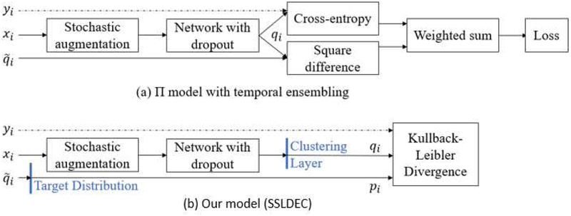
Figure 1 shows our proposed model (SSLDEC) compared to the Π model with temporal ensembling [11]. As can be seen, our method shares similarities with the self-ensembling methods discussed Section II as at each epoch, we compute a target distribution p_i based on the predictions of the network and use it to reduce the difference between this prediction and another prediction computed from the same input but with different data augmentation. Network dropout is also used in both models to improve consistency and robustness in network parameter optimization. The main difference between our model and the Π model and its variations is that we added a clustering layer in the penultimate layer of the network. The implication of this is that while the Π model evaluates the network outputs twice in the same way, we use a different target distribution which aims to create more accurate clusters by a powerful training algorithm for SSLDEC that is described next.

Fig. 1.

(a) The Π model with temporal ensembling as described in [11]; and (b) our model (SSLDEC) that, compared to the Π model, has an additional clustering layer instead of a dense layer with a softmax activation, where a prediction is passed through a target distribution as explained in equation (3). While the Π model uses weighted sum of cross-entropy and squared difference between predictions, our model uses Kullback-Leibler divergence as the loss for both labeled and unlabeled data points as described in Section III-B. Both models use stochastic data augmentation and network dropout for regularization.

B. The Training Algorithm

To train SSLDEC we need to define a target distribution for the unlabeled points. Similar to DEC, this distribution should have the following properties:

• Increase the purity of each cluster

• Put more emphasis over points with high confident predictions

• Prevent one large cluster to distort the embedding space

Therefore, following [6], we define this distribution as:

$$p_{i,j}=\frac{q_{i,j}^2/f_j}{\sum _{j^{\prime }}{q}_{i,j^{\prime }}^2/f_{j^{\prime }}},$$ (2)

with f_j = ∑_i q_i,j. The square term over q is added to increase the purity of the clusters, and the frequencies f are designed to prevent distortion from large clusters.

Also following [6] and similar to the parametric t-SNE algorithm [35] we use the Kullback-Leibler (KL) divergence as a loss function to compare target (P) and embedding (Q) probability distributions:

$$\begin{gathered} D_{KL}(P\Vert Q)=\sum _i\sum _j{p}_{i,j}log\left(\frac{p_{i,j}}{q_{i,j}}\right) \\ =\sum _i\sum _j{p}_{i,j}log\left(p_{i,j}\right)-\sum _i\sum _j{p}_{i,j}log\left(q_{i,j}\right) \\ =-H(P)+H(P,Q) \end{gathered}$$ (3)

In a supervised learning task, this function is equivalent to the commonly used cross-entropy. In other words, if the true distribution P is fixed, as in a supervised framework, then the entropy H(P) is constant, and the KL divergence is equivalent to the cross-entropy. In semi-supervised training, our goal is to match the predictions to the target distribution, and thus the KL divergence is suitable as, although not a distance, it is a measure of divergence between two distributions.

Algorithm 1 presents our training method, which involves pretraining using labeled data for 100 epochs, followed by iterations of making predictions using labeled and unlabeled data, computing target distributions through equation (2), selecting a balanced subset of P, and training the model with the balanced subset until an accuracy condition meets. The selection of this balanced subset P′ is based on predictions from the algorithm. We select the same number of samples whose prediction given by the neural network is one of each label. The total number of selected labels, therefore, depends on the minimum of samples whose predictions are one particular label. The algorithm uses standard backpropagation to compute parameters and gradients of the clustering layer as well as those of the CNN. For the clustering layer, the gradients of the loss L associated with the cluster centers μ and the embeddings z follow these equations:

$$\begin{gathered} \frac{\partial L}{\partial z_i}=2\sum _j{\left(1+\Vert z_i-{\mu }_j{\Vert }^2\right)}^{-1}\times \left(p_{i,j}-q_{i,j}\right)\left(z_i-{\mu }_j\right) \\ \frac{\partial L}{\partial {\mu }_j}=-2\sum _i{\left(1+\Vert |z_i-{\mu }_j{\Vert }^2\right)}^{-1}\times \left(p_{i,j}-q_{i,j}\right)\left(z_i-{\mu }_j\right) \end{gathered}$$ (4)

These gradients are then passed to the CNN.

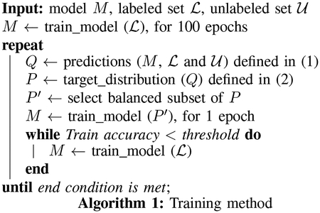
The training of the model is performed in two parts. We first pretrain it using only the available labeled data. Despite using only a relatively small set of labeled data, this part has significant influence on the results, as the target distribution defined in equation (2) is based on the output of this pretraining, which, therefore, needs to be as accurate as possible. During this pretraining, the loss of the CNN is the KL divergence between q and an empirical distribution obtained from the labeled data. Moreover, the centroids of the clustering layer, randomly initialized, are also trained along with the rest of the algorithm. Then we train the CNN using every data point. In this part, we repeat a cycle of two training steps. The first step involves training the algorithm with labeled and unlabeled data using target distributions as true labels, and the second step involves training the network using only the labeled data until a training accuracy score is achieved. During the training step using the target distribution, we randomly select a balanced subset of the data to avoid one class distorting the embedding space.

Here we explain the rationale behind using the second step of training using the labeled data only. During the two-step training process the algorithm makes mistakes and corrects them. Indeed, during the second part of the training, the algorithm is trained using pseudo-labels, even when true labels are available, therefore it is prone to making mistakes. If the mis-classification rate is too large, it is possible that some of the labeled data will be misclassified as well. Retraining the network with only labeled points can correct these classification mistakes, and the combination of the training steps in Algorithm 1 ultimately results in a more accurately trained model. As a result, after each epoch of training using unlabeled data, we retrain the network with the labeled points until the training accuracy reaches a certain level, which we choose to be 100% on the labeled training data. This choice of 100% accuracy was empirically made, and can induce overfitting if the labeled set is relatively large compared to the unlabeled dataset. However, in typical semi-supervised learning scenarios when the labeled set is much smaller than the unlabeled set, it is possible to reach 100% accuracy on labeled data without a risk of overfitting.

IV. Experiments

To evaluate the performance of our proposed method (SSLDEC), we performed several experiments on various benchmark datasets under standard experimental conditions where we were able to compare our results with the results reported by other semi-supervised learning methods. In particular, we applied our method to the following datasets:

• Two half moons drawn using the Sklearn package [36]

• The MNIST dataset, consisting of 70,000 hand written digits [5],

• The SVHN, consisting of around 125,000 pictures of digits from street house numbers [37],

• The iSeg, consisting of 3D T1-weighted (T1w) and T2-weighted (T2w) brain MRI scans of 23 six-month old infants as part of the iSeg2017 challenge [1]. Brain tissue segmentation in iSeg is challenging as gray matter and white matter appear with isointensity values on both T1w and T2w MRI scans around six months of age.

We used the half moons data for illustration, the MNIST and SVHN as standard image classification benchmarks, and the iSeg as a medical image segmentation task. In this section, first we present the network architectures for the classification and segmentation tasks, and then describe the details of the experimental setup and results for each experiment.

A. SSLDEC network for image classification

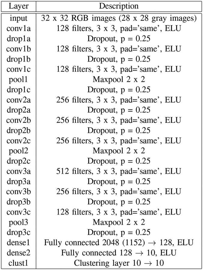
For image classification using SSLDEC, we used a CNN with the architecture presented in Figure 2 for every image classification experiment except the half moon test. This network consists of 9 convolutional layers, followed by 2 dense layers and by the clustering layer shown in Figure 1. Each convolutional and fully connected layer has a batch normalization unit, along with an exponential linear unit (ELU) activation function [38]. We also applied a L₂ kernel regularization with weight 10⁻⁴ on every convolutional and dense layer. In this network, the last layer does not have any softmax activation layer, as the clustering layer returns normalized probabilities for each sample.

Fig. 2.

Description of the CNN architecture used in all classification experiments except the two half moons experiment. Dropout was used after every convolutional layer, and a clustering layer shown in Figure 1 was added to the top of the network. ELU: exponential linear unit.

We trained this network by feeding it with batches of samples of size 128, and used the Adam optimizer function [39] with common settings (β₁ = 0.9, β₂ = 0.999). As described in Section III-A we used the KL divergence as our loss, and trained the network with Algorithm 1 in two steps: first the network was pretrained using only labeled data for 100 epochs in a supervised setting to initialize the clusters, and second it was trained iteratively by using all labeled and unlabeled data samples along with computing target distribution based on equation (2). We used a learning rate that linearly decayed from 10⁻³ to 10⁻⁴ during the pretraining, and a steady learning rate of 10⁻⁴ for the second part of the training. Finally, for this classification problem, we used an ensemble of five models to improve generalization on unlabeled data and boost the performance of the algorithm.

B. SSLDEC network for 3D image segmentation

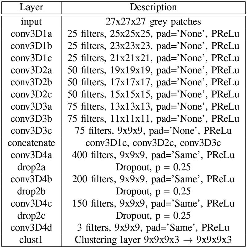
For 3D medical image segmentation and its application to iSeg, we implemented SSLDEC on a 3D fully convolutional CNN with forward skip connections from convolutional layers to fully connected layers based on [40], which resembles a 3D densely connected network [41] with 3 blocks of 3 convolutional layers. These blocks are followed by 3 fully connected layers and a last layer which is our clustering layer defined before (also see Figure 1). The input of the network is a patch of size 27×27×27, and the output is of size 9×9×9, as the dimension is progressively reduced due to a choice of not including any padding in the convolutional layers. The full segmentation network architecture is shown in Figure 3.

Fig. 3.

Description of the densely connected 3D CNN architecture with 3 dense blocks used for 3D image segmentation. A clustering layer shown in Figure 1 was added to the top of the network. In this application the clustering layer was applied to every voxel instead of the whole image for the segmentation task. PReLu: parametric rectified linear unit.

As Figure 3 shows, the first 9 convolutional layers are grouped in 3 dense blocks. Each convolutional layer is followed by a batch normalization layer and a parametric rectified linear unit (PReLu) activation function [42]. We did not include any padding for these layers, so the size of each output decreases from patches of sizes 27 × 27 × 27 to sizes 9 × 9 × 9. The outputs of all dense blocks are concatenated and added to 3 additional convolutional layers along with batch normalization, PReLu activation and dropout. The top of the network involved our clustering layer. As opposed to the clustering layer in the classification network, which discriminates whole images, the clustering layer of the segmentation network discriminates each voxel. As a result, the input and the output of this layer is 9 × 9 × 9 × 3, corresponding respectively to the size of a patch (9 × 9 × 9) and to the number of labels (3 labels for the iSeg challenge corresponding to grey matter, white matter, and cerebrospinal fluid).

C. Half Moons

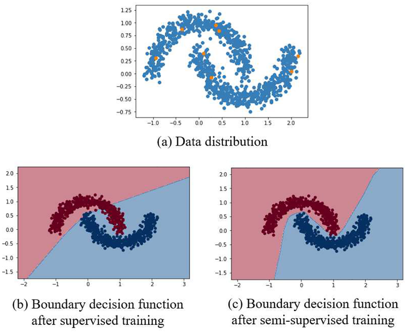
In this section, we show a simple demonstration of SSLDEC in action applied to the half-moons dataset. In this test, we drew 1000 points from a two half-moons distribution using the python package Sklearn [36], with a noise standard deviation of 0.1. We randomly selected 4 points from each half-moon as labeled data, and considered the rest of the points as unlabeled data. In this section only, our CNN consisted of 4 dense layers of size 10 with RELU activation function, followed by one dense layer of size 2 and a clustering layer. Figure 4 shows the decision boundary of our model after training the algorithm only with the labeled data, and after SSLDEC training; which shows that SSLDEC was able to recover the underlying distribution of the two half moons after using the unlabeled data.

Fig. 4.

Simple test of our semi-supervised algorithm (SSLDEC) using a two-half-moons distribution. (a) Data distribution: 8 labeled points (orange points, 4 of each label) were used as labeled training data and the rest (blue points) were considered unlabeled data; (b) decision boundary after supervised training with labeled data; (c) decision boundary after SSLDEC. The accuracy score after SSLDEC reached 99.8%.

This simple experiment meant to display the advantage of the proposed semi-supervised method compared to supervised-only training with limited data. Separating the two half moons using a limited amount of points is considered a hard problem and the results depend on the number and position of the labeled points. In our experiments we observed that by using a total of 8 points (4 of each label) fairly distributed over the dataset, SSLDEC could accurately find the decision boundary and achieve a high accuracy.

D. MNIST

The hand-written digits database, MNIST [5], has been widely used as a standard benchmark to compare semi-supervised learning algorithms. This dataset consists of 70,000 small images, among which 10,000 are used as the test set. Following the standard semi-supervised learning experiments with this dataset, we randomly selected 100 (and 1000) images, 10 (and 100) of each class, of the training set as labeled data, and used the rest of the training data as unlabeled samples. For this classification task, we used moderate data augmentation through small translations of one pixel along the width and the height of each image. We found, experimentally, that using this augmentation to draw different predictions from the same input generated better results than computing the prediction of a noisy input.

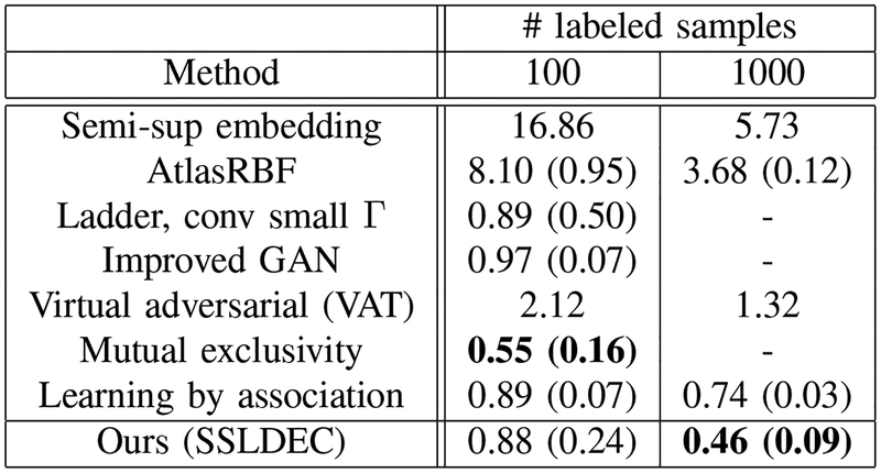
Following standard evaluation criteria for semi-supervised learning, we randomly selected 10 different subsets, and reported mean accuracy score on the test set along with its standard deviation reported in brackets. Figure 5 presents our results as well as the results of several recent semi-supervised methods for labeled sets of size 100 and 1000. Our method generated competitive results on this dataset, particularly outperforming [16] using a labeled dataset of size 1000.

Fig. 5.

MNIST results for 100 and 1000 labeled samples for training, compared with Semi-supervised embedding [15], AtlasRBF [43], the Ladder network [9], Improved GAN [44], Virtual adversarial training (VAT) [45], Mutual exclusivity [10] and Learning by association [16]. The best results in each column are shown in bold text.

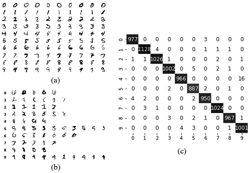
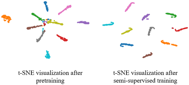
Figures 6 and 7 illustrate sample results and the performance of our proposed semi-supervised method (SSLDEC) on MNIST classification. Figure 6 displays the training set along with some misclassified examples, as well as the confusion matrix on the test set. Among the misclassified images, many can be stated as ambiguous for a human annotator. Figure 7 displays the 10 clusters recovered by the classification network after the pre-training stage (with labeled data) and after our semi-supervised method (SSLDEC). This figure shows how the initial clusters were refined after semi-supervised training leading to very small misclassification rate (very few data points were associated to a wrong cluster).

Fig. 6.

Sample results of our MNIST classification: (a) labeled samples; (b) mis-classified samples from the test set; and (c) confusion matrix of the test set. In this test, the accuracy score was 99.28%.

Fig. 7.

t-SNE visualization of 1000 data points from the MNIST dataset after pretraining the network using 100 labeled data (left), and after iterations of our semi-supervised training algorithm (right).

E. SVHN

SVHN [37] is a real-world image dataset consisting of pictures of house numbers separated as digits. The task associated with this dataset is therefore to classify each of these numbers as a digit, similar to MNIST. This dataset differs from MNIST in two main aspects: it is significantly larger, containing around 125,000 images, and its classes are slightly imbalanced, as the frequency of classes (1,2,3) appears to be higher than the other digits. In training classification networks we used the same data augmentation that we used for MNIST: translations of one pixel along both directions.

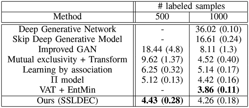
SVHN has also been used as a standard benchmark for semi-supervised methods, where 500 and 1000 samples from the training set are used as labeled data and the rest of the training data are used as unlabeled samples. Figure 8 presents our results for the SVHN dataset. Similar to the MNIST dataset, we report the mean accuracy score of 10 different experiments as well as its standard deviation, reported in brackets. These results show that our method outperformed most of the other methods tested on the same dataset, with the exception of the VAT with 1000 labeled points. Note that on MNIST our method outperformed VAT by a large margin (Figure 5). Also note that while our method did not perform as well as “mutual exclusivity” [10] on MNIST, it outperformed mutual exclusivity by a margin on SVHN. Considered all together, the results on both MNIST and SVHN datasets, presented in Figures 5 and 8, indicate that our technique performed better than other semi-supervised learning algorithms in these image classification tasks.

Fig. 8.

SVHN results for 500 and 1000 labeled samples in the training set, compared with semi-supervised learning with Deep generative network (DGN) [46], Skip Deep Generative Model [47], Improved GAN [44], Mutual exclusivity [10], Learning by association [16], the model [11] and the VAT model [13]. The best results in each column are shown in bold text.

F. Isointense infant brain MRI segmentation

Segmenting brain MRI of infants to white matter (WM), gray matter (GM), and cerebrospinal fluid (CSF) when infants are at around 6 months of age is extremely challenging because the T1 and T2 relaxation times of the WM and GM tissue of the rapidly myelinating brain at this age are similar and thus these tissues appear as isointense regions on both T1w and T2w MRI scans. This motivated the recent iSeg2017 challenge that involves T1w and T2w pairs of MRI scans of 23 infants scanned at around 6 months old. The tissues were manually segmented for all cases by a neuroradiologist [1]. MRI scans of 10 subjects constitute the training set that is available along with their manual segmentations, and the rest of the subjects remain for test. Only challenge organizers have access to the manual labels for the 13 test subjects.

We used iSeg training and test data to evaluate our semi-supervised learning method (SSLDEC) for segmentation. To train our 3D densely connected CNN with SSLDEC, we randomly selected a subset of the training dataset in three scenarios: from the training set of 10 images, we only kept one fifth of 1, 2, and 5 images to draw labeled training samples. For semi-supervised learning we used the rest of the unlabeled training and test data to improve the performance of the CNN using SSLDEC, following the training algorithm described in Section III. We tested the trained model on the 5 cases from the iSeg training set that were not used as labeled data in training as well as on iSeg test data.

We compared SSLDEC results against two supervised-only settings: one using the labeled training set used in each SSLDEC trained model as defined above (i.e. using only one fifth of 1, 2, and 5 cases). This defined the lower bound baseline model; and another using full labeled training images (i.e. 1, 2, and 5 full images). This was considered the baseline for higher bound performance on full labeled images. We also compared our method against a pseudo-labelling method, which was implemented using our segmentation network without the clustering layer and thus without computing the target distribution. We refer to these methods as lower bound, higher bound, and pseudo labeling model in our results.

To evaluate segmentation we computed the Dice score for every class (tissue type in iSeg), which is defined as

$$\text{Dice}=\frac{2*TP}{2*TP+FP+FN}$$

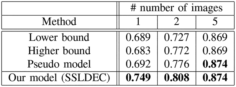
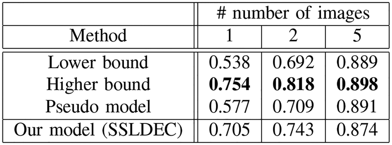
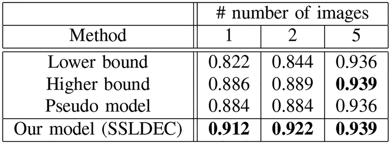
where TP, FP and FN represent the true positive, false positive and false negative rates, respectively. The average of Dice scores over the test set for three experiments (with 1, 2, and 5 labeled images for training) is shown in Figures 9, 10 and 11, for WM, GM, and CSF classes, respectively. The results show that for the WM and CSF classes SSLDEC achieved better results than the higher bound and the pseudo model, especially with a large margin in training with only 1 and 2 images. Note that the higher bound model used 5 times more number of labeled samples for training than SSLDEC. For GM which was more difficult to segment (due to its narrow boundaries and shape and isointense appearance with WM), SSLDEC results did not reach as high level of accuracy as the higher bound model, but exceeded the accuracy obtained from both lower bound and pseudo models by a large margin in experiments with 1 and 2 labeled images.

Fig. 9.

Dice scores for white (WM) matter segmentation, compared with the lower and higher bound trained models, and the pseudo-labelling semi-supervised method for experiments with 1, 2, and 5 labeled training images. For WM segmentation our method outperformed all other models including the higher bound model which used full labeled images instead of only using one-fifth of the labels of each training image.

Fig. 10.

Dice scores for grey matter (GM), compared with the lower and higher bound trained models, and the pseudo-labelling semi-supervised method for experiments with 1, 2, and 5 labeled training images. For GM segmentation, which is more challenging due to the narrow boundaries and shape of the cortex, our method outperformed the lower bound and pseudo models in experiments with 1 and 2 labeled images, but did not reach as high accuracy as the higher bound model.

Fig. 11.

Dice scores for the cerebrospinal fluid (CSF) segmentation, compared with the lower and higher bound trained models and the pseudo-labelling semi-supervised method for experiments with 1, 2, and 5 labeled training images. For CSF segmentation our method outperformed all other models including the higher bound model which used full labeled images instead of only using one-fifth of the labels of each training image.

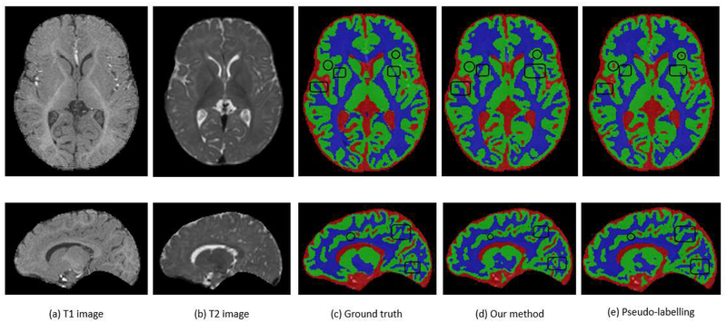
Overall, the results of these experiments show that a high level of accuracy can be achieved by labelling only one-tenth of the original data and using the rest of the data as unlabeled samples, which using our proposed algorithm improved the performance of a pretrained supervised-only model significantly. On official iSeg test data, by using only one-fifth of the slices of each training image as labeled data and using the rest of the training and test images as unlabeled data, we obtained Dice scores of 93.7%, 88.8% and 86.3% for CSF, GM, and WM, respectively, compared to 94.8%, 90.6% and 88.5% for the fully-supervised model trained on all training data. Figure 12 shows sample axial and sagittal slices of T1w and T2w images as well as segmentations of a case from the test set (the 6th case in the iSeg training data that was used as a test case in our study), comparing our semi-supervised method (SSLDEC) using one fifth of 2 images as the labeled training data, with segmentation obtained from the pseudo-labelling method and the ground truth (manual segmentation provided by challenge organizers). This figure shows that our method (SSLDEC) provided fairly accurate segmentation of WM, GM, and CSF in this challenging application by using a small fraction of the labeled training data, as it outperformed the pseudo-labelling method in most areas.

Fig. 12.

Results of (d) our model (SSLDEC) on a case from the isointense infant brain MRI segmentation challenge (iSeg), compared to (c) the ground truth (manual segmentation) and (e) a pseudo-labelling technique. Original T1- and T2-weighted MRI images of this case are also displayed in (a) and (b) which show the difficulty in distinguishing WM and GM due to their isointensity appearance at this age. These slices were extracted from image 6 on the iSeg dataset, after training models on one fifth of 2 images only (images 1 and 2 in the iSeg dataset). These results show that the pseudo-labelling technique includes several CSF zones, which are not present in the ground truth or in the results of our semi-supervised technique (black circles). Overall, SSLDEC also seems to be more accurate in separating gray and white matters as several WM zones are correctly linked by our SSLDEC model, whereas not by the pseudo-labelling technique (black rectangles). There are areas in which the pseudo-labelling segmentation seems more similar to ground truth than SSLDEC segmentation, but the overall results show that SSLDEC outperformed pseudo-labelling in this case and other cases, as confirmed by average Dice scores obtained and reported in Figures 9, 10, and 11. The average Dice score (over the three classes) of the SSLDEC model for this case was 89.3%, while it was 87.5% for the pseudo-labelling technique.

V. Discussion and Conclusion

We have proposed a novel semi-supervised learning method, utilizing the powerful deep embedded clustering approach, that can be easily used with any neural network. This method achieved competitive results for the classification of small 2D images using a classification network as well as accurate voxelwise segmentation of 3D medical images using a densely connected fully convolutional neural network. Moreover, this method did not require a large validation set to tune hyper-parameters. This is considered a huge advantage over many state-of-the-art semi-supervised deep learning algorithms, where the dependency on large validation sets to adjust hyper-parameters is considered a disadvantage as it is contrary to the motivation behind the design of semi-supervised learning methods [9], [48]. In fact, we used the same network for every experiment made for image classification, along with the same optimizer and learning rate and achieved results that, overall, were better than state-of-the-art semi-supervised learning methods. Our proposed semi-supervised learning method (SSLDEC) inherits its robustness and minimal need for hyper-parameter tuning from the deep embedded clustering algorithm [6].

Our results in image classification and segmentation indicate that the performance of supervised-only methods with limited number of labeled training samples can be significantly improved by using the proposed semi-supervised learning algorithm. This method, therefore, has the potential to enhance applications of deep learning in areas where data labeling is costly and time-consuming, such as medical image segmentation. It can reduce the amount of data samples and the time experts need to spend to label samples or voxels to generate training data. In Section II-B we briefly mentioned techniques other than semi-supervised learning that can help reduce the need for labeling large amounts of data for deep learning. In particular, we referred to transfer learning and active learning approaches. In some very interesting future extensions, our proposed method (SSLDEC) may be adopted and used for transfer learning, where a CNN is pre-trained using large labeled data in one domain and then trained with unlabeled and labeled data in a target domain. SSLDEC may also be combined with active learning to query most informative unlabeled samples to be labeled by an expert, thus effectively taking advantage of both semi-supervised learning (using unlabeled data) as well as active learning.

References

- [1].Wang L, Li G, Lin W, and Shen D. (2017) 6-months infant brain MRI segmentation. [Online]. Available: http://iseg2017.web.unc.edu/
- [2].LeCun Y, Bengio Y, and Hinton G, “Deep learning,” nature, vol. 521, no. 7553, p. 436, 2015. [DOI] [PubMed] [Google Scholar]
- [3].Goodfellow I, Bengio Y, Courville A, and Bengio Y, Deep learning. MIT press Cambridge, 2016, vol. 1. [Google Scholar]
- [4].Hinton GE and Salakhutdinov RR, “Reducing the dimensionality of data with neural networks,” science, vol. 313, no. 5786, pp. 504–507, 2006. [DOI] [PubMed] [Google Scholar]
- [5].LeCun CCY and Burges CJ., “The mnist database of handwritten digits,” 1998.
- [6].Xie J, Girshick R, and Farhadi A, “Unsupervised deep embedding for clustering analysis,” in International conference on machine learning, 2016, pp. 478–487. [Google Scholar]
- [7].Lee D-H, “Pseudo-label: The simple and efficient semi-supervised learning method for deep neural networks,” in Workshop on Challenges in Representation Learning, ICML, vol. 3, 2013, p. 2. [Google Scholar]
- [8].Zhou Z-H and Li M, “Tri-training: Exploiting unlabeled data using three classifiers,” IEEE Transactions on knowledge and Data Engineering, vol. 17, no. 11, pp. 1529–1541, 2005. [Google Scholar]
- [9].Rasmus A, Berglund M, Honkala M, Valpola H, and Raiko T, “Semi-supervised learning with ladder networks,” in Advances in Neural Information Processing Systems, 2015, pp. 3546–3554. [Google Scholar]
- [10].Sajjadi M, Javanmardi M, and Tasdizen T, “Regularization with stochastic transformations and perturbations for deep semi-supervised learning,” in Advances in Neural Information Processing Systems, 2016, pp. 1163–1171. [Google Scholar]
- [11].Laine S and Aila T, “Temporal ensembling for semi-supervised learning,” arXiv preprint arXiv:1610.02242, 2016. [Google Scholar]
- [12].Tarvainen A and Valpola H, “Mean teachers are better role models: Weight-averaged consistency targets improve semi-supervised deep learning results,” in Advances in neural information processing systems, 2017, pp. 1195–1204. [Google Scholar]
- [13].Miyato T, Maeda S.-i., Ishii S, and Koyama M, “Virtual adversarial training: a regularization method for supervised and semi-supervised learning,” IEEE transactions on pattern analysis and machine intelligence, 2018. [DOI] [PubMed] [Google Scholar]
- [14].Ranzato M and Szummer M, “Semi-supervised learning of compact document representations with deep networks,” in Proceedings of the 25th international conference on Machine learning. ACM, 2008, pp. 792–799. [Google Scholar]
- [15].Weston J, Ratle F, Mobahi H, and Collobert R, “Deep learning via semi-supervised embedding,” in Neural Networks: Tricks of the Trade. Springer, 2012, pp. 639–655. [Google Scholar]
- [16].Haeusser P, Mordvintsev A, and Cremers D, “Learning by association-a versatile semi-supervised training method for neural networks,” in IEEE Conference on Computer Vision and Pattern Recognition (CVPR), vol. 3, no. 5, 2017, p. 6. [Google Scholar]
- [17].van Rikxoort E, Galperin-Aizenberg M, Goldin J, Kockelkorn T, van Ginneken B, and Brown M, “Multi-classifier semi-supervised classification of tuberculosis patterns on chest ct scans,” in The Third International Workshop on Pulmonary Image Analysis, 2010, pp. 41–48. [Google Scholar]
- [18].Wang B, Liu KW, Prastawa KM, Irima A, Vespa PM, Van Horn JD, Fletcher PT, and Gerig G, “4d active cut: An interactive tool for pathological anatomy modeling,” in Biomedical Imaging (ISBI), 2014 IEEE 11th International Symposium on. IEEE, 2014, pp. 529–532. [DOI] [PMC free article] [PubMed] [Google Scholar]
- [19].Feng Z, Nie D, Wang L, and Shen D, “Semi-supervised learning for pelvic mr image segmentation based on multi-task residual fully convolutional networks,” in Biomedical Imaging (ISBI 2018), 2018 IEEE 15th International Symposium on. IEEE, 2018, pp. 885–888. [DOI] [PMC free article] [PubMed] [Google Scholar]
- [20].Moradi E, Pepe A, Gaser C, Huttunen H, Tohka J, Initiative ADN et al. , “Machine learning framework for early mri-based alzheimer’s conversion prediction in mci subjects,” Neuroimage, vol. 104, pp. 398–412, 2015. [DOI] [PMC free article] [PubMed] [Google Scholar]
- [21].An L, Adeli E, Liu M, Zhang J, and Shen D, “Semi-supervised hierarchical multimodal feature and sample selection for Alzheimers disease diagnosis,” in International Conference on Medical Image Computing and Computer-Assisted Intervention. Springer, 2016, pp. 79–87. [DOI] [PMC free article] [PubMed] [Google Scholar]
- [22].Mahapatra D, “Semi-supervised learning and graph cuts for consensus based medical image segmentation,” Pattern Recognition, vol. 63, pp. 700–709, 2017. [Google Scholar]
- [23].Gu L, Zheng Y, Bise R, Sato I, Imanishi N, and Aiso S, “Semi-supervised learning for biomedical image segmentation via forest oriented super pixels (voxels),” in International Conference on Medical Image Computing and Computer-Assisted Intervention. Springer, 2017, pp. 702–710. [Google Scholar]
- [24].Van Opbroek A, Ikram MA, Vernooij MW, and De Bruijne M, “Transfer learning improves supervised image segmentation across imaging protocols,” IEEE transactions on medical imaging, vol. 34, no. 5, pp. 1018–1030, 2015. [DOI] [PubMed] [Google Scholar]
- [25].Tajbakhsh N, Shin JY, Gurudu SR, Hurst RT, Kendall CB, Gotway MB, and Liang J, “Convolutional neural networks for medical image analysis: Full training or fine tuning?” IEEE transactions on medical imaging, vol. 35, no. 5, pp. 1299–1312, 2016. [DOI] [PubMed] [Google Scholar]
- [26].Hoo-Chang S, Roth HR, Gao M, Lu L, Xu Z, Nogues I, Yao J, Mollura D, and Summers RM, “Deep convolutional neural networks for computer-aided detection: Cnn architectures, dataset characteristics and transfer learning,” IEEE transactions on medical imaging, vol. 35, no. 5, p. 1285, 2016. [DOI] [PMC free article] [PubMed] [Google Scholar]
- [27].Ghafoorian M, Mehrtash A, Kapur T, Karssemeijer N, Marchiori E, Pesteie M, Guttmann CR, de Leeuw F-E, Tempany CM, van Ginneken B et al. , “Transfer learning for domain adaptation in mri: Application in brain lesion segmentation,” in International Conference on Medical Image Computing and Computer-Assisted Intervention. Springer, 2017, pp. 516–524. [Google Scholar]
- [28].Litjens G, Kooi T, Bejnordi BE, Setio AAA, Ciompi F, Ghafoorian M, Van Der Laak JA, Van Ginneken B, and Sánchez CI, “A survey on deep learning in medical image analysis,” Medical image analysis, vol. 42, pp. 60–88, 2017. [DOI] [PubMed] [Google Scholar]
- [29].Yang L, Zhang Y, Chen J, Zhang S, and Chen DZ, “Suggestive annotation: A deep active learning framework for biomedical image segmentation,” in International Conference on Medical Image Computing and Computer-Assisted Intervention. Springer, 2017, pp. 399–407. [Google Scholar]
- [30].Sourati J, Gholipour A, Dy JG, Kurugol S, and Warfield SK, “Active deep learning with fisher information for patch-wise semantic segmentation,” in Deep Learning in Medical Image Analysis and Multimodal Learning for Clinical Decision Support. Springer, 2018, pp. 83–91. [DOI] [PMC free article] [PubMed] [Google Scholar]
- [31].Cheplygina V, de Bruijne M, and Pluim JP, “Not-so-supervised: a survey of semi-supervised, multi-instance, and transfer learning in medical image analysis,” arXiv preprint arXiv:1804.06353, 2018. [DOI] [PubMed] [Google Scholar]
- [32].Hou C, Nie F, Yi D, and Tao D, “Discriminative embedded clustering: A framework for grouping high-dimensional data,” IEEE transactions on neural networks and learning systems, vol. 26, no. 6, pp. 1287–1299, 2015. [DOI] [PubMed] [Google Scholar]
- [33].Huang P, Huang Y, Wang W, and Wang L, “Deep embedding network for clustering,” in Pattern Recognition (ICPR), 2014 22nd International Conference on. IEEE, 2014, pp. 1532–1537. [Google Scholar]
- [34].Maaten L. v. d. and Hinton G, “Visualizing data using t-sne,” Journal of machine learning research, vol. 9, no. Nov, pp. 2579–2605, 2008. [Google Scholar]
- [35].Maaten L, “Learning a parametric embedding by preserving local structure,” in Artificial Intelligence and Statistics, 2009, pp. 384–391. [Google Scholar]
- [36].Buitinck L, Louppe G, Blondel M, Pedregosa F, Mueller A, Grisel O, Niculae V, Prettenhofer P, Gramfort A, Grobler J, Layton R, VanderPlas J, Joly A, Holt B, and Varoquaux G, “API design for machine learning software: experiences from the scikit-learn project,” in ECML PKDD Workshop: Languages for Data Mining and Machine Learning, 2013, pp. 108–122. [Google Scholar]
- [37].Netzer Y, Wang T, Coates A, Bissacco A, Wu B, and Ng AY, “Reading digits in natural images with unsupervised feature learning,” in NIPS workshop on deep learning and unsupervised feature learning, vol. 2011, no. 2, 2011, p. 5. [Google Scholar]
- [38].Clevert D-A, Unterthiner T, and Hochreiter S, “Fast and accurate deep network learning by exponential linear units (elus),” arXiv preprint arXiv:1511.07289, 2015. [Google Scholar]
- [39].Kingma DP and Ba J, “Adam: A method for stochastic optimization,” CoRR, vol. abs/1412.6980, 2014. [Online]. Available: http://arxiv.org/abs/1412.6980 [Google Scholar]
- [40].Dolz J, Desrosiers C, and Ayed IB, “3d fully convolutional networks for subcortical segmentation in mri: A large-scale study,” NeuroImage, 2017. [DOI] [PubMed] [Google Scholar]
- [41].Huang G, Liu Z, Van Der Maaten L, and Weinberger KQ, “Densely connected convolutional networks” in CVPR, vol. 1, no. 2, 2017, p. 3. [Google Scholar]
- [42].He K, Zhang X, Ren S, and Sun J, “Delving deep into rectifiers: Surpassing human-level performance on imagenet classification,” CoRR, vol. abs/1502.01852, 2015. [Online]. Available: http://arxiv.org/abs/1502.01852 [Google Scholar]
- [43].Pitelis N, Russell C, and Agapito L, “Semi-supervised learning using an unsupervised atlas,” in Joint European Conference on Machine Learning and Knowledge Discovery in Databases. Springer, 2014, pp. 565–580. [Google Scholar]
- [44].Salimans T, Goodfellow I, Zaremba W, Cheung V, Radford A, and Chen X, “Improved techniques for training gans,” in Advances in Neural Information Processing Systems, 2016, pp. 2234–2242. [Google Scholar]
- [45].Miyato T, Maeda S.-i., Koyama M, Nakae K, and Ishii S, “Distributional smoothing with virtual adversarial training,” arXiv preprint arXiv:1507.00677, 2015. [Google Scholar]
- [46].Kingma DP, Mohamed S, Rezende DJ, and Welling M, “Semi-supervised learning with deep generative models,” in Advances in Neural Information Processing Systems, 2014, pp. 3581–3589. [Google Scholar]
- [47].Maaløe L, Sønderby CK, Sønderby SK, and Winther O, “Auxiliary deep generative models,” arXiv preprint arXiv:1602.05473, 2016. [Google Scholar]
- [48].Oliver A, Odena A, Raffel C, Cubuk ED, and Goodfellow IJ, “Realistic evaluation of deep semi-supervised learning algorithms,” arXiv preprint arXiv:1804.09170, 2018. [Google Scholar]