

Abstract
Purpose:
We evaluated muscle/fat fraction (MFF) accuracy and reliability measured with an MR imaging technique at 1.5 Tesla (T) and 3.0 T scanner strengths, using biopsy as reference.
Methods:
MRI was performed on muscle samples from pig and rabbit species (n = 8) at 1.5 T and 3.0 T. A chemical shift based 2-point Dixon method was used, collecting in-phase and out-of-phase data for fat/water of muscle samples. Values were compared to MFFs calculated from histology.
Results:
No significant difference was found between 1.5 and 3.0 T (P values = 0.41 – 0.96), or between histology and imaging (P = 0.83) for any muscle tested.
Conclusion:
Results suggest that a 2-point Dixon fat/water separation MRI technique may provide reliable quantification of MFFs at varying field strengths across different animal species, and consistency was established with biopsy. The results set a foundation for larger scale investigation of quantifying muscle-fat in neuromuscular disorders.
Keywords: MRI, muscle imaging, muscle fat infiltrates, muscle-fat, muscle/fat fraction
Introduction
Muscle fat infiltration (MFI) has been both observed qualitatively and measured quantitatively with magnetic resonance imaging (MRI) in a number of neuromusculoskeletal pathologies1–5. MRI is widely accepted as the gold standard for measuring changes in soft-aqueous skeletal muscle, such as markers of muscle denervation (longer T1 and T2 relaxation times due to cellular fluid changes)6, and such measures have been validated7. For example, physiological alterations in muscle tissue, measured as signal intensity ratios using short time to inversion recovery MRI, have been shown to be consistent with electrophysiological evidence of denervation and renervation7.
Accordingly, MRI may hold prognostic potential in a myriad of disease processes where denervation or neurological decline may drive the clinical course8 (e.g. spinal cord injury9, muscular dystrophy10, spinal muscular atrophy11, rotator cuff tears12, and whiplash injury13). However, the accuracy of both the qualitative and quantitative metrics of MRI when applied to skeletal muscle imaging and MFI calculation has yet to be validated comprehensibly.
Challenges for the consistent quantification of MFI exist due to the variety of MRI scanners worldwide that differ in field strength. Furthermore, MR acquisition methods vary for detection of fat and water. We have used and reported a simple approach for determining the magnitude of MFI in patients with neck pain following whiplash injury1,13, and in keeping with the advancements in imaging, we have expanded our quantification of MFI by using fat/water separation techniques14,15. Because markers of MFI may hold promise for determining the stage, progression, and response to management of neurological disease, the external validation of such findings must be established via comparison of different scanner strengths using a similar data acquisition method referenced to the gold standard, muscle biopsy.
Therefore, the purpose of this preliminary study was to assess the reliability of MRI for quantifying MFI with muscle/fat fractions (MFF) with a 2-point Dixon method at 2 field strengths (1.5 and 3.0T), using samples from 2 different species of skeletal muscle tissue (pig and rabbit), and to validate via the reference standard, biopsy/histology.
Materials and Methods
Pig Muscle Imaging:
The initial tissue specimen utilized in this study was harvested from a fresh pig carcass. The cut was made to include the skin, subcutaneous fat, muscle compartments, vertebral bodies, and spinal cord of the lower cervical and upper thoracic region of the carcass.
The tissue was imaged in the 1.5 T and 3.0 T scanners within 1 hour of being obtained. The specifics of the pulse sequence and set-up for imaging in each of the scanners were: 3D gradient echo, chemical shift based 2 point Dixon method using the standard head coil. The 1.5 T protocol details were: acquisition time (TA) = 4:21, resolution = 0.7 × 0.7 × 3 mm, field of view (FOV) = 320 × 190 mm, echo times (TE/TE2) = 2.39/4.77 ms, repetition time (TR)= 6.79 ms, 6 averages, flip angle = 120, 36 slices, bandwidth = 510 Hz/px. The 3.0 T protocol details were: TA = 4:23, resolution = 0.7 × 0.7 × 3 mm, FOV = 320 × 190 mm, TE/TE2/TR = 2.45/3.675/6.59 ms, 6 averages, flip angle = 120, 36 slices, bandwidth = 510 Hz/px.
Analysis of the MR imaging was performed post-hoc using Analyze 11.0 software (AnalyzeDirect, Mayo Clinic, Rochester MN) by 2 investigators experienced in MFF quantification and stored on a secured laptop computer. Measurements for each scanner were taken at 4 locations of the sample: the right and left rhomboideus cervicus muscles (RRC, LRC), and the right and left paraspinal muscles (RP, LP). A vitamin E tablet was secured at each muscle measurement location and used as an anatomical reference for all scans (Figure 1). The defined regions of interest (ROIs) were performed in these 4 muscles by outlining each muscle within its fascial borders at the same locations with both the in-and opposed-phase sequences using a 3 mm slice thickness. The MFF is a unitless ratio of fat signal intensity to fat plus water signal intensity, and these MFFs were created using the equation: Relative Fat Signal/ (Relative Water + Relative Fat Signal) * 100. Averages were taken over 3 consecutive slices to form the MFFs.
Figure 1:

ROIs were taken by outlining each muscle within its fascial borders at the same points simultaneously using the water (panel A) and fat-weighted (panel B) images. The box outline corresponds to the muscle measured, and the outline in the bottom right section of panel A highlights the vitamin E tablet attached as a spatial reference.
After establishing the methodology for comparing skeletal muscle tissue between the 2 scanner strengths, validation was sought by referencing histological analyses.
Rabbit Muscle Imaging:
Four skeletal muscle samples were harvested from the rabbit to be used for histological analysis (2 from the cervical spine region and 2 from the left lower extremity thigh region).
The rabbit was imaged at both 1.5 T and 3.0 T using the same methods as detailed for the pig. The MR analysis was performed in the same manner as above.
Histology Methods:
An investigator with 16 years of experience supervised and assisted with all stages of the muscle biopsy and subsequent histological preparation. The rabbit muscle tissue from the 4 locations was harvested as 2 cc samples, then fresh frozen and cut into 5 μm slices for slide preparation. High-resolution images were recorded at the cellular level using the HistoFAXS Tissue Analysis System (TissueGnostics USA, Tarzana, CA) and analyzed using a customized imaging program created in MatLab (MathWorks, Natick, MA). Hematoxylin and eosin stain (H & E) staining causes muscle cells to appear in a red hue and fat cells to appear opaque white. The muscle and fat cells were profiled using color channel analysis. A region labeling routine was then performed to profile the fat cells, whereby each region was classified with the empirically determined parameters of area and color, pertaining to fat cells or empty space. ROI analysis was implemented to measure the histological MFFs.
Fat regions observed using the H & E technique were cross checked and verified by obtaining a second sample located 5 μm from the H & E and staining with Oil Red O. This stain utilizes a fat-soluble dye, and when it is applied to the sample, regional lipids appear bright red. Figure 2 illustrates the method utilized to ensure accurate muscle and fat measurement with the histology data.
Figure 2:
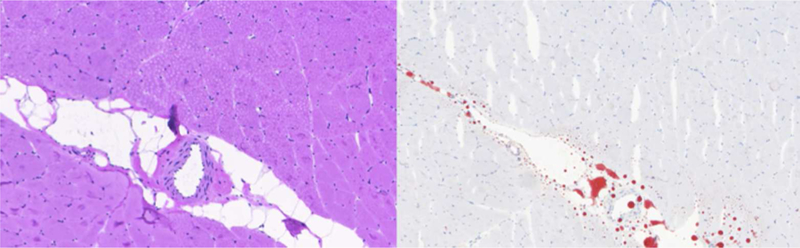
The MFFs were calculated with the custom color channel analysis program using H & E stains (left), and lipid regions were cross-referenced using Oil Red O stains (right).
Statistical Analysis
All statistical analyses were completed using MatLab (MathWorks, Natick, MA). A two-sample Kolmogorov-Smirnov test was conducted to ensure all measurements were from the same continuous distribution, and thus, parametric testing was appropriate. For the pig data, a one-way analysis of variance (ANOVA) with multiple comparison of means post-hoc testing (Tukey-b) was chosen to test for any statistically significant differences between the 4 muscles. With 3 slices per each of the 4 muscles across 2 scanner strengths, the ANOVA was performed on a 3 × 8 matrix. The rabbit data were analyzed in the same fashion.
To analyze the histological portion of the study, 2 separate investigators calculated MFFs independently. A one-way ANOVA with multiple comparison of means post-hoc testing (Tukey-b) was conducted on these values from both raters compared to the averages of the 1.5 T and 3.0 T measures for the 4 muscles sampled (a 4 × 4 matrix).
Reliability of Imaging Methodology:
Two independent raters measured each of the 4 rabbit and 4 pig muscle ROIs according to the methods described above. An intra-class correlation coefficient (ICC 3,1) between these 2 measurements was chosen to establish a measure of inter-rater reliability. Similarly, rater 1 also repeated measurements to establish intra-rater reliability, and an intra-class correlation coefficient (ICC 3,1) was chosen for this metric. Bland-Altman plots were created to demonstrate rater agreement. P < 0.05 was considered significant for all statistical tests.
Results
Imaging Data:
Kolmogorov-Smirnov tests met the assumption of homogeneity for both the pig and rabbit samples (P = 0.19 and P = 0.43, respectively). No significant difference was found between the 2 scanner strengths for any of the 4 ROIs tested in the pig (P = 0.41). The averages for the percent fat at 1.5 T and 3.0 T were 5.61 ± 0.46 and 5.79 ± 0.26, respectively. The results are summarized in Table 1 and Figure 3. Figure 4 is a Bland-Altman plot demonstrating the level of agreement between the 1.5T and 3.0T scanners for the pig sample.
Table 1:
Pig Muscle/Fat Fractions (MFF)
| Muscle | 1.5T Mean MFF | 3.0T Mean MFF |
|---|---|---|
| RRC | 4.94 ± 0.54 | 5.37 ± 0.05 |
| LRC | 6.16 ± 0.21 | 6.07 ± 0.38 |
| RP | 5.86 ± 0.91 | 5.88 ± 0.34 |
| LP | 5.47 ± 0.99 | 5.85 ± 0.13 |
(P = 0.41 for the ANOVA test)
Figure 3:
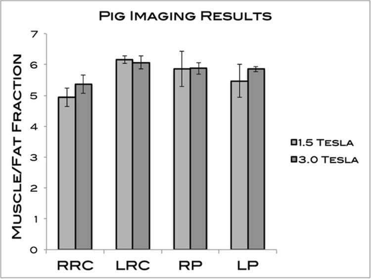
MFFs of the 4 pig muscles measured. The averages for 1.5T and 3.0T were 5.61 ± 0.46 and 5.79 ± 0.26, respectively. No significant differences were found.
Figure 4:
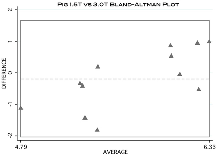
Bland-Altman plot visually demonstrating the level of agreement of MFF calculation between 1.5T and 3.0T scanners using the pig data.
Additionally, no significant difference was found between the 2 scanner strengths for any of the rabbit muscles tested (P = 0.96). The averages for the percent fat at 1.5 T and 3.0 T were 4.32 ± 0.27 and 4.29 ± 0.35, respectively. The results are summarized in Table 2 and Figure 5. The Bland-Altman plot demonstrates the level of agreement between 1.5T and 3.0T scanners for the rabbit sample (Figure 6).
Table 2:
Rabbit Muscle/Fat Fractions (MFF)
| Muscle | 1.5T Mean MFF | 3.0T Mean MFF |
|---|---|---|
| Neck 1 | 4.21 ± 0.63 | 4.12 ± 0.55 |
| Neck 2 | 4.46 ± 0.51 | 3.88 ± 1.19 |
| Leg 1 | 3.94 ± 0.10 | 4.84 ± 0.83 |
| Leg 2 | 4.67 ± 0.29 | 4.30 ± 1.93 |
(P = 0.96 for the ANOVA test)
Figure 5:
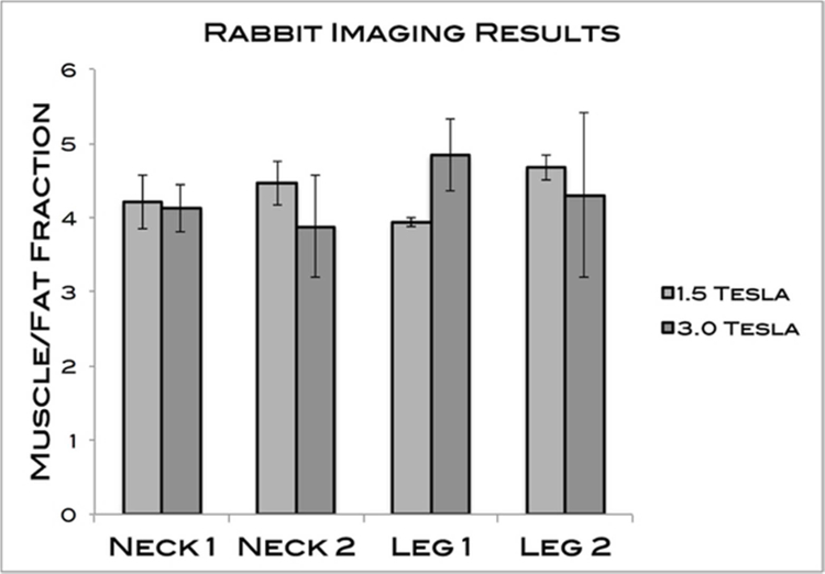
MFFs of the 4 rabbit muscles measured. The averages for 1.5T and 3.0T were 4.32 ± 0.27 and 4.29 ± 0.35, respectively. No significant differences were found.
Figure 6:
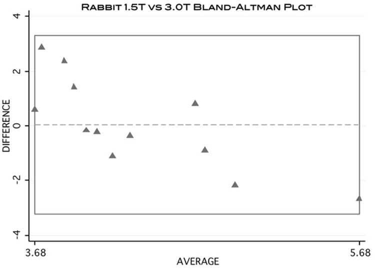
Bland-Altman plot visually demonstrating the level of agreement of MFF calculation between 1.5T and 3.0T scanners using the rabbit data.
Histological Data:
Table 3 and Figure 7 summarize the histological data analysis compared to MRI. The average standard deviation between the 2 raters was 0.06, indicating an appropriate level of reliability of the color channel analysis. No significant differences were found between the histological measures and the imaging methods for any of the 4 muscles tested (P = 0.83). The averages for rabbit histology and MRI were 4.00 ± 0.11 and 4.28 ± 0.29, respectively.
Table 3:
Rabbit MRI versus Histology
| Muscle | 1.5T Mean MFF | 3.0T Mean MFF | Rater 1 Histology | Rater 2 Histology |
|---|---|---|---|---|
| Neck 1 | 4.21 ± 0.05 | 4.12 ± 0.05 | 3.94 ± 0.03 | 4.01 ± 0.03 |
| Neck 2 | 4.46 ± 0.29 | 3.88 ± 0.29 | 3.97 ± 0.05 | 4.08 ± 0.05 |
| Leg 1 | 3.94 ± 0.45 | 4.84 ± 0.45 | 4.02 ± 0.09 | 4.20 ± 0.09 |
| Leg 2 | 4.67 ± 0.29 | 4.30 ± 1.93 | 3.94 ± 0.06 | 3.81 ± 0.06 |
(P = 0.83 for the ANOVA test)
Figure 7:
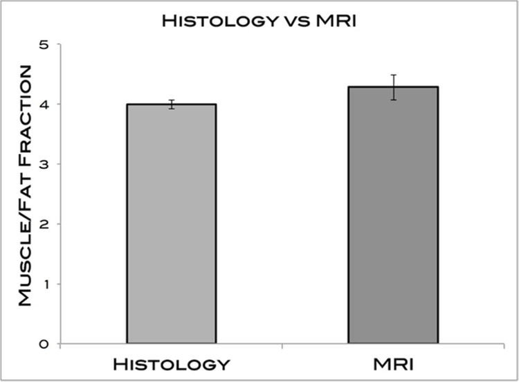
MFFs of MRI and histology measures. The averages for histology and MRI were 4.00 ± 0.11 and 4.28 ± 0.29, respectively. No significant differences were found.
Inter-rater Reliability of Imaging Methodology:
The calculated ICC (3,1) = 0.77 indicated a reasonably strong level of agreement between the investigators. The Bland-Altman plot demonstrates the level of agreement between the 2 raters (Figure 8).
Figure 8:
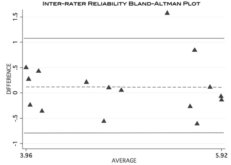
Bland-Altman plot visually demonstrating the level of agreement of MFF calculation between 2 separate raters using the MRI data.
Intra-rater Reliability of Imaging Methodology:
The calculated ICC (3,1) = 0.64, indicated a moderate level of agreement. Figure 9 is a Bland-Altman plot demonstrating the level of intra-rater agreement.
Figure 9:
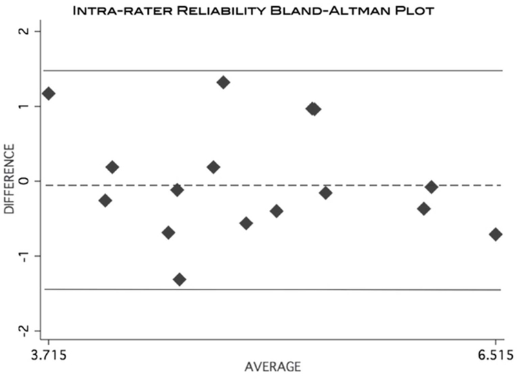
Bland-Altman plot visually demonstrating the level of agreement of MFF calculation from a single rater taking repeated measurements using the MRI data.
Discussion
This study demonstrates that muscle-fat MR imaging bears no statistically significant differences across field strengths (1.5T and 3.0T) for samples obtained from 2 different animal species. Despite encouraging preliminary findings, the results should be interpreted with caution, considering a small sample of muscles was measured (n=8), and standard deviations were relatively high (0.05 – 1.93). Other studies have compared MR imaging at 1.5T and 3.0T field strengths in cardiac research, multiple sclerosis, pre-operative wrist pain, pancreatitis and pancreatic cancer, prostate cancer, rheumatoid arthritis, and brain tumor, but these investigations did not focus on muscle-fat quantification16–28.
Similar to others29, our results indicate that MFFs measured using a Dixon Fat/Water separation MRI technique were consistent with histological measurements. Utilizing a different approach compared to Gaetta and colleagues29, we controlled for the location of imaging measurement using vitamin E tablets in the MRI field of view, and by cross-verifying histological regions of fat by using Oil Red O slides.
In addition, the muscle-fat MR imaging protocol appears reliable with repeated measures and across investigators. Earlier research has found excellent ICC inter and intra-rater levels of reliability with MR imaging for muscle-fat quantification (ICC = 0.94 and 0.93, respectively) using T1-weighted imaging1, but radio frequency slice profiles have evolved and there is a strong call to utilize more advanced standardized MR-based imaging methods for quantifying tissue fat concentration30.
Recent evidence using a 3D multi-echo gradient echo Dixon based method for muscle-fat quantification in the human neck found comparable results to T1-weighted imaging.14 Other researchers used a similar multi-echo technique and found comparable results to spectroscopy31. However, the latter study focused on the investigation of liver fat fractions, which can be affected by the presence of iron and motion artifacts. This is not the case in ex vivo muscle samples or in vivo muscle imaging, and although we initially experimented with an 8-point Dixon technique, we found the 2-point Dixon method to be sufficient due to the lack of susceptibility effects from iron. Using this two-echo method within the specific anatomical environment of skeletal muscle offers higher resolution, shorter acquisition time, and better signal-to-noise compared to multi-echo.
Other MR methods are commonly used for enhancing the contrast of fat and water, including Short TI Inversion Recovery (STIR) sequences, which employ inversion times during which the fat spins will not contribute to the resulting image32. While clinically useful for fat nullification in order to observe potential lesions, these inversion recovery sequences are not practical for muscle-fat quantification due to the difficulty in measuring a definitive fat signal. We have also explored the use of single voxel magnetic resonance spectroscopy, but we found the time constraints (6 minute acquisition time per 10 mm3 volume) and the demand for a high quality magnetic shim were restrictive. Also, although the fat signal possesses a spectrum with multiple peaks, the 2-point Dixon method focuses on the largest peak, which is shifted ≈ 3.5 parts per million from the water peak and accounts for the majority of the fat signal energy33. We believe that by focusing on this dominant portion of the fat signal, the 2-point Dixon method is the optimal method for skeletal muscle-fat quantification, compared to multi-echo or spectroscopy.
Limitations:
One should note that it is difficult to standardize the location of the MFF ROIs with H & E staining techniques. While there is a certain level of subjectivity on where the MFFs should be generated, best efforts were made to address this by using the Oil Red O images as a cross-reference. Furthermore, a common histological artifact may be caused with tissue spreading during sample preparation, which produces an appearance visually similar to fat cells. Accordingly, we calibrated our custom color-channel histological analysis with MatLab for quantification of fat cells, while removing any/all of the potential larger areas that could be due to tissue spreading.
A second inherent limitation is that, although Oil Red O slides were used to verify fat regions on the H&E slides, the prepared samples are separated by only 5 microns. Accordingly, an exact overlay of images for precise comparison was not possible.
Further, the histological images and the MR images are not of equal scale. The slices analyzed are a small portion of the volume of the MRI voxel, and assumptions of generalizability were made.
Finally, although our omnibus testing (ANOVAs) yielded no statistically significant differences, some of the individual muscles tested displayed descriptive variability that was relatively large in magnitude. For example, the right rhomboideus cervicus muscle from the pig measured a greater standard deviation using the 1.5T scanner (0.54) compared to the 3.0T scanner (0.05). In other instances, the 3.0T measurements had higher standard deviations. According to our preliminary data, MFF values varied from 0.05 to 1.93 using the 2-point Dixon technique. Future investigations should consistently co-register the images to ensure that the anatomy of interest is representative across field strengths, as this may improve accuracy.
Conclusion
This preliminary study demonstrates quantification of animal muscle-fat using commonly available MR field strengths. Furthermore, the use of a simple 2-point Dixon method may provide an accurate measure for MFF. Moreover, this imaging protocol is both reliable and valid. As such, researchers, radiologists, and other interested clinicians can have a certain level of confidence that the use of this tool for quantifying MFI in human neuromusculoskeletal disorders is suitable. This work is currently underway in our laboratory.
Acknowledgements
The pig specimen was generously donated by the staff at Peoria Packing. The following facilities at Northwestern University (NU) played important roles in the data collection of this study: NU Mouse Histology and Phenotyping Laboratory, NU Cell Imaging Facility, NU Center for Translational Imaging, and NU Translational Interventional and Oncologic Imaging Group. Andrew C. Smith is supported by the NIH-funded Training Program in the Neurobiology of Movement and Rehabilitation Sciences at Northwestern University, supported by the Eunice Kennedy Shriver National Institute Of Child Health & Human Development Grant T32 HD057845. Funding for the study was provided by internal sources and James Elliott is supported by the National Center for Research Resources (NCRR) and the Northwestern University Clinical and Translational Sciences Institute (NUCATS), NIH KL2 RR025740.
Abbreviations
- MFF
muscle/fat fraction
- T
Tesla
- MRI
magnetic resonance imaging
- MFI
muscle fatty infiltrates
- TA
acquisition time
- FOV
field of view
- TE
echo time
- TR
repetition time
- RRC and LLC
right and left rhomboideus cervicus muscles
- RP and LP
right and left paraspinal muscles
- ROI
region of interest
- H & E
hematoxylin and eosin stain
- ANOVA
analysis of variance
- ICC
intra-class correlation coefficient
- NU
Northwestern University
Footnotes
Publisher's Disclaimer: This article has been accepted for publication and undergone full peer review but has not been through the copyediting, typesetting, pagination and proofreading process which may lead to differences between this version and the Version of Record.
References
- 1.Elliott JM, Jull G, Noteboom JT, Darnell R, Galloway G, Gibbon WW. Fatty infiltration in the cervical extensor muscles in persistent whiplash-associated disorders: a magnetic resonance imaging analysis. Spine 2006;31(22):E847–55. [DOI] [PubMed] [Google Scholar]
- 2.Samagh SP, Kramer EJ, Melkus G, Laron D, Bodendorfer B, Natsuhara K, et al. MRI quantification of fatty infiltration and muscle atrophy in a mouse model of rotator cuff tears. J Orthop Res 2013;31(3):421–6. [DOI] [PubMed] [Google Scholar]
- 3.Alizai H, Nardo L, Karampinos DC, Joseph G, Yap S, Baum T, et al. Comparison of clinical semi-quantitative assessment of muscle fat infiltration with quantitative assessment using chemical shift-based water/fat separation in MR studies of the calf of post-menopausal women. Eur Radiol 2012;22(7):1592–600. [DOI] [PMC free article] [PubMed] [Google Scholar]
- 4.Wokke BH, Bos C, Reijnierse M, van Rijswijk C, Eggers H, Webb A, et al. Comparison of dixon and T1-weighted MR methods to assess the degree of fat infiltration in duchenne muscular dystrophy patients. J Magn Reson Imaging 2013;000:1–6. [DOI] [PubMed] [Google Scholar]
- 5.Ryan AS, Dobrovolny CL, Smith G V, Silver KH, Macko RF. Hemiparetic muscle atrophy and increased intramuscular fat in stroke patients. Arch Phys Med Rehabil 2002;83(12):1703–7. [DOI] [PubMed] [Google Scholar]
- 6.Fleckstein J, Watumull D, Conner K, Ezaki M, Greenlee RG, Bryan WW, et al. Denervated human skeletal muscle: MR imaging evaluation. Radiology 1993;187:213–218. [DOI] [PubMed] [Google Scholar]
- 7.McDonald CM, Carter GT, Fritz RC, Anderson MW, Abresch RT, Kilmer DD. Magnetic resonance imaging of denervated muscle: comparison to electromyography. Muscle Nerve 2000;23(9):1431–4. [DOI] [PubMed] [Google Scholar]
- 8.Holl N, Echaniz-Laguna A, Bierry G, Mohr M, Loeffler JP, Moser T, et al. Diffusion-weighted MRI of denervated muscle: a clinical and experimental study. Skeletal Radiol 2008;37(12):1111–7. [DOI] [PubMed] [Google Scholar]
- 9.Gorgey S, Dudley G. Skeletal muscle atrophy and increased intramuscular fat after incomplete spinal cord injury. Spinal Cord 2007;45(4):304–9. [DOI] [PubMed] [Google Scholar]
- 10.Gaeta M, Messina S, Mileto A, Vita G, Ascenti G, Vinci S, et al. Muscle fat-fraction and mapping in Duchenne muscular dystrophy: evaluation of disease distribution and correlation with clinical assessments. Preliminary experience. Skeletal Radiol 2012;41(8):955–61. [DOI] [PubMed] [Google Scholar]
- 11.Mercuri E, Messina S, Kinali M, Cini C, Longman C, Battini R, et al. Congenital form of spinal muscular atrophy predominantly affecting the lower limbs: a clinical and muscle MRI study. Neuromuscul Disord 2004;14(2):125–129. [DOI] [PubMed] [Google Scholar]
- 12.Goutallier D, Postel J- M, Gleyze P, Leguilloux P, Van Driessche S. Influence of cuff muscle fatty degeneration on anatomic and functional outcomes after simple suture of full-thickness tears. J Shoulder Elb Surg 2003;12(6):550–554. [DOI] [PubMed] [Google Scholar]
- 13.Elliott JM, Pedler A, Kenardy J, Galloway G, Jull G, Sterling M. The temporal development of fatty infiltrates in the neck muscles following whiplash injury: an association with pain and posttraumatic stress. PLoS One 2011;6(6):e21194. [DOI] [PMC free article] [PubMed] [Google Scholar]
- 14.Elliott JM, Walton DM, Rademaker A, Parrish TB. Quantification of cervical spine muscle fat: a comparison between T1-weighted and multi-echo gradient echo imaging using a variable projection algorithm (VARPRO). BMC Med Imaging 2013;13(1):30. [DOI] [PMC free article] [PubMed] [Google Scholar]
- 15.Elliott JM, Kerry R, Flynn T, Parrish TB. Content not quantity is a better measure of muscle degeneration in whiplash. Man Ther 2013:1–5. [DOI] [PubMed] [Google Scholar]
- 16.Michaely HJ, Nael K, Schoenberg SO, Laub G, Reiser MF, Finn JP, et al. Analysis of cardiac function--comparison between 1.5 Tesla and 3.0 Tesla cardiac cine magnetic resonance imaging: preliminary experience. Invest Radiol 2006;41(2):133–40. [DOI] [PubMed] [Google Scholar]
- 17.Anderson ML, Skinner J, Felmlee JP, Berger R, Amrami KK. Diagnostic comparison of 1.5 Tesla and 3.0 Tesla preoperative MRI of the wrist in patients with ulnar-sided wrist pain. J Hand Surg Am 2008;33(7):1153–9. [DOI] [PubMed] [Google Scholar]
- 18.Bachmann R, Reilmann R, Schwindt W, Kugel H, Heindel W, Krämer S. FLAIR imaging for multiple sclerosis: a comparative MR study at 1.5 and 3.0 Tesla. Eur Radiol 2006;16(4):915–21. [DOI] [PubMed] [Google Scholar]
- 19.Sicotte NL, Voskuhl RR, Bouvier S, Klutch R, Cohen MS, Mazziotta JC. Comparison of multiple sclerosis lesions at 1.5 and 3.0 Tesla. Invest Radiol 2003;38(7):423–7. [DOI] [PubMed] [Google Scholar]
- 20.Cheng ASH, Pegg TJ, Karamitsos TD, Searle N, Jerosch-Herold M, Choudhury RP, et al. Cardiovascular magnetic resonance perfusion imaging at 3-tesla for the detection of coronary artery disease: a comparison with 1.5-tesla. J Am Coll Cardiol 2007;49(25):2440–9. [DOI] [PubMed] [Google Scholar]
- 21.Biswas J, Nelson CB, Runge VM, Wintersperger BJ, Baumann SS, Jackson CB, et al. Brain Tumor Enhancement in Magnetic Resonance Imaging. Invest Radiol 2005;40(12):792–797. [DOI] [PubMed] [Google Scholar]
- 22.Nöbauer-Huhmann IM, Ba-Ssalamah A, Mlynarik V, Barth M, Schöggl A, Heimberger K, et al. Magnetic resonance imaging contrast enhancement of brain tumors at 3 tesla versus 1.5 tesla. Invest Radiol 2002;37(3):114–9. [DOI] [PubMed] [Google Scholar]
- 23.Edelman RR, Salanitri G, Brand R, Dunkle E, Ragin A, Li W, et al. Magnetic Resonance Imaging of the Pancreas at 3.0 Tesla. Invest Radiol 2006;41(2):175–180. [DOI] [PubMed] [Google Scholar]
- 24.Sosna J, Pedrosa I, Dewolf WC, Mahallati H, Lenkinski RE, Rofsky NM. MR imaging of the prostate at 3 Tesla: comparison of an external phased-array coil to imaging with an endorectal coil at 1.5 Tesla. Acad Radiol 2004;11(8):857–62. [DOI] [PubMed] [Google Scholar]
- 25.Shellock FG, Tkach J a., Ruggieri PM, Masaryk TJ. Cardiac pacemakers, ICDs, and loop recorder: evaluation of translational attraction using conventional (“long-bore”) and “short-bore” 1.5 and 3.0 Tesla MR systems. J Cardiovasc Magn Reson 2003;5(2):387–397. [DOI] [PubMed] [Google Scholar]
- 26.Yang P, Nguyen P, Shimakawa A, Brittain J, Pauly J, Nishimura D, et al. Spiral magnetic resonance coronary angiography: direct comparison of 1.5 Tesla vs. 3 Tesla. J Cardiovasc Magn Reson 2004;6(4):877–884. [DOI] [PubMed] [Google Scholar]
- 27.Hinton DP, Wald LL, Pitts J, Schmitt F. Comparison of cardiac MRI on 1.5 and 3.0 Tesla clinical whole body systems. Invest Radiol 2003;38(7):436–42. [DOI] [PubMed] [Google Scholar]
- 28.Wieners G, Detert J, Streitparth F, Pech M, Fischbach F, Burmester G, et al. High-resolution MRI of the wrist and finger joints in patients with rheumatoid arthritis: comparison of 1.5 Tesla and 3.0 Tesla. Eur Radiol 2007;17(8):2176–82. [DOI] [PubMed] [Google Scholar]
- 29.Gaeta M, Scribano E, Mileto A, et al. Muscle fat fraction in neuromuscular disorders: dual-echo dual-flip-angle spoiled gradient-recalled MR imaging technique for quantification--a feasibility study. Radiology 2011;259(2):487–94. [DOI] [PubMed] [Google Scholar]
- 30.Reeder SB, Hu HH, Sirlin CB. Proton density fat-fraction: a standardized MR-based biomarker of tissue fat concentration. J Magn Reson Imaging 2012;36(5):1011–4. [DOI] [PMC free article] [PubMed] [Google Scholar]
- 31.Kühn J- P, Hernando D, Mensel B, Krüger P, Ittermann T, Mayerle J, et al. Quantitative chemical shift-encoded MRI is an accurate method to quantify hepatic steatosis. J Magn Reson Imaging 2013;00:1–8. [DOI] [PMC free article] [PubMed] [Google Scholar]
- 32.Bydder G, Young I. MR imaging: clinical use of the inversion recovery sequence. J Comput Assist Tomogr. 1985;9:659–675. [PubMed] [Google Scholar]
- 33.Brix G, Heiland S, Bellemann M, Koch T, Lorenz W. MR imaging of fat-containing tissues: valuation of two quantitative imaging techniques in comparison with localized proton spectroscopy. Magn Reson Imaging. 1993;11:977–991. [DOI] [PubMed] [Google Scholar]