Computation of Object Approach by a Wide-Field, Motion-Sensitive Neuron

Abstract

The lobula giant motion detector (LGMD) in the locust visual system is a wide-field, motion-sensitive neuron that responds vigorously to objects approaching the animal on a collision course. We investigated the computation performed by LGMD when it responds to approaching objects by recording the activity of its postsynaptic target, the descending contralateral motion detector (DCMD). In each animal, peak DCMD activity occurred a fixed delay δ (15 ≤ δ ≤ 35 msec) after the approaching object had reached a specific angular threshold θ_thres on the retina (15° ≤ θ_thres ≤ 40°). θ_thres was independent of the size or velocity of the approaching object. This angular threshold computation was quite accurate: the error of LGMD and DCMD in estimating θ_thres(3.1–11.9°) corresponds to the angular separation between two and six ommatidia at each edge of the expanding object on the locust retina. It was also resistant to large amplitude changes in background luminosity, contrast, and body temperature. Using several experimentally derived assumptions, the firing rate of LGMD and DCMD could be shown to depend on the product ψ(t − δ) · e^{−αθ(t−δ)}, where θ(t) is the angular size subtended by the object during approach, ψ(t) is the angular edge velocity of the object and the constant, and α is related to the angular threshold size [α = 1/tan(θ_thres/2)]. Because LGMD appears to receive distinct input projections, respectively motion- and size-sensitive, this result suggests that a multiplication operation is implemented by LGMD. Thus, LGMD might be an ideal model to investigate the biophysical implementation of a multiplication operation by single neurons.

The processing of sensory information by neural circuits is known to depend critically on the implementation of nonlinear operations. Multiplication, for example, is thought to be the elementary building block underlying the detection of visual motion in insects (Reichardt, 1987; Borst and Egelhaaf, 1989) or the generation of gain fields in posterior parietal neurons of the primate neocortex (Andersen et al., 1985). Despite years of efforts, the precise biophysical and network mechanisms underlying these nonlinear operations remain elusive (Koch and Poggio, 1992). Here, we study two identified locust visual neurons, which may prove well suited to investigate the biophysical implementation of a multiplication operation.

The lobula giant motion detector (LGMD) belongs to a class of neurons sometimes called “jittery movement detectors” (Glantz, 1974;Frantsevich and Mokrushov, 1977, for review, see Wehner, 1981). Its dendritic arborizations ramify in the third neuropil (lobula) of the locust optic lobes and consist of three dendritic subfields (O’Shea and Williams, 1974). The main subfield is thought to receive in part an excitatory retinotopic projection, which is sensitive to motion, whereas the remaining two dendritic subfields receive massive feed-forward inhibitory inputs, which are size-dependent (Palka, 1967;Rowell et al., 1977). In contrast to directionally selective neurons involved in optomotor response behaviors and gaze stabilization, such as those extensively studied in the fly visual system (Hausen and Egelhaaf, 1989), LGMD is inhibited by whole field motion (Pinter, 1977;Zaretsky and Rowell, 1979). It responds to movement of small objects, irrespective of their location in its receptive field, in a nondirectionally selective way. It is also vigourously excited by objects approaching on a collision course with the animal (Schlotterer, 1977; Rind and Simmons, 1992). In the locust brain, both left and right LGMD neurons each synapse onto one descending contralateral motion detector (DCMD) neuron, whose fast-conducting axon, the largest in the contralateral nerve cord, projects to thoracic motor centers involved in the generation of jump and flight maneuvers (Burrows and Rowell, 1973; Pearson et al., 1980; Simmons, 1980; Robertson and Pearson, 1983). The connection between LGMD and DCMD is very strong and reliable such that each action potential in LGMD elicits an action potential in DCMD. Conversely, under visual stimulation, each action potential in DCMD is caused by an action potential in LGMD (O’Shea and Williams, 1974; Rind, 1984). These anatomical and physiological properties suggest that LGMD and DCMD are part of an early warning system aimed at eliciting escape or avoidance behaviors in face of an imminent danger.

Although the preferential response of LGMD and DCMD to looming objects on a collision course with the animal has been recognized for some time (Schlotterer, 1977; Rind and Simmons, 1992), the neural computation performed by LGMD during approach remained unclear. The experiments and theoretical analysis presented here were aimed at understanding this computation and the algorithm used to perform it (Marr, 1982). A part of our results has been published recently (Hatsopoulos et al., 1995) but has been criticized on the basis of the low refresh rate of the monitor used in those experiments (Rind and Bramwell, 1996, note added in proof; Judge and Rind, 1997; Rind and Simmons, 1997). In addition to confirming our original findings, the present work shows that the peak in DCMD activity depends solely on the retinal image size of the approaching object. It also provides a better theoretical foundation for our results by deriving from a few plausible assumptions a model describing the firing rate of LGMD and DCMD in response to approaching objects. This model generalizes that of Hatsopoulos et al. (1995); its free parameters are determined experimentally.

MATERIALS AND METHODS

Preparation. Experiments were performed on adult locusts (mostly female) taken from the laboratory colony 3–4 weeks after their final molt. Locusts were mounted dorsal side-up on a plastic holder, which was then fixed vertically to a clamp located directly under a dissection microscope. The head of the locust was placed between the jaws of an alligator clip mounted on a micromanipulator and was carefully aligned with reference points marked on a reticular grid inserted in one of the microscope eyepieces. After alignment, the head was fixed in place with a few drops of beeswax. This, together with the calibration procedure described below, allowed us to reliably align the center of the locust’s right eye with the center of our stimulation screen. A small piece of rigid plastic paper (transparency film; Eastman Kodak, Rochester, NY) cut to fit the dimensions of the outer edge of the locust’s eye was glued in place as close as possible to the anterior rim of the right eye with fast epoxy glue. A waterproof wax cup terminating on this plastic sheet was then built around the locust’s head. In some experiments no plastic sheet was used, and the wax cup was built directly up to the rim of the eye. The entire dorsal half of the head was bathed in locust saline (Laurent and Davidowitz, 1994), except for the right eye, which remained outside the cup formed by the plastic sheet and the wax, with an unobstructed field of view of at least 100° measured from the center of the eye.

The brain (supraoesophageal ganglion) and the optic lobes were exposed by opening a rectangular window in the frontal head cuticle. The gut was removed to minimize coupling of abdominal respiratory movements to the brain and to expose the connectives. The suboesophageal ganglion was grabbed with a pair of fine forceps, and both connectives were sectioned as close as possible to the suboesophageal ganglion. In a few of the experiments reported here, locusts were also prepared for simultaneous intracellular recordings from the dendrites or axon of LGMD by desheating the right optic lobe with fine forceps after softening the protective sheet surrounding the brain with protease (XIV; Sigma, St. Louis, MO). The results of these experiments will be reported elsewhere.

Electrophysiology and data acquisition. The locust was fixed to a clamp with its longitudinal body axis parallel to the stimulation screen, and the cut end of the proximal, left connective (contralateral to the stimulated eye) was placed in a suction electrode. Extracellular signals were amplified with a differential AC amplifier (A-M Systems, Everett, WA) and recorded using a digital tape recorder (Micro Data Instruments, Woodhaven, NY; sampling rate, 11.5 kHz) together with the transistor-transistor logic (TTL) synchronization pulses generated by the computer controlling the stimulation screen. DCMD typically produced the largest action potentials in the nerve cord and was easily identified from its characteristic responses to small objects moving in the visual field of the animal or to looming stimuli (see Fig. 2). The preparation was sometimes allowed to recover from the dissection for 15–30 min before starting an experiment, and stable recordings from DCMD could be maintained up to 4 hr, depending on the robustness of the animal and the quality of the dissection.

Fig. 2.

Extracellular recording from DCMD in response to object approach (l/‖v‖ = 45 msec). Top panel, Time course of size of the approaching object on the stimulation screen, as monitored by TTL synchronization pulses. Bottom panel, Extracellular recording from the contralateral connective, showing DCMD as the largest unit. Note the short interruption in spiking during approach (curved arrow). Thick,thin solid lines, dashed line, Estimate of the instantaneous firing frequency obtained by smoothing the response with 20, 15, and 10 msec Gaussian windows, respectively. *Peak firing rate. Note that in this example, peak firing time is not determined with great certainty because of the two local maxima separated by the short interruption (arrow). For this experiment, l/‖v‖ = 45 msec was the least favorable stimulus parameter to estimate the peak, as can be seen from the error bars for the point l/‖v‖ = 45 msec in Figure 4A. Left inset, 20 msec Gaussian window used to smooth the spike rasters (same horizontal time scale as the extracellular trace, not drawn to scale in the vertical direction). spk, Spike.

Stimulus generation. Visual stimuli were generated on a monochrome monitor coated with an ultrafast P46 phosphor (10% decay time, 1 μsec; Vision Research Graphics, Durham, NH) emitting in the green–yellow range (normalized intensity reaching >95% between 520 and 565 nm and >50% between 505 and 610 nm), close to the peak in the absorption spectrum of locust photoreceptors (Lillywhite, 1978; Osorio, 1986a). The monitor image was refreshed at a rate of 200 Hz, well above the temporal cutoff frequency of locust photoreceptors (<100 Hz;Miall, 1978; Howard, 1981; Howard et al., 1984). The monitor was placed at a distance of 120 mm from the center of the locust’s eye. Alignment of the center of the locust’s eye with the center of the monitor and distance adjustment were achieved by (1) leveling horizontally and vertically the monitor and the air table supporting the clamp for the preparation, and (2) placing a locust with the head fixed to its holder (see Preparation above) in the clamp and adjusting the distance and eye position with respect to the monitor with the help of an optical bench consisting of two 10 mW helium–neon lasers and two reflection mirrors (Uniphase, Manteca, CA).

The dimensions of the image were 300 × 209 mm (736 × 500 pixels) corresponding to a spatial resolution of 5 pixel/° at the center of the locust’s eye [spatial resolution of the locust ommatidial array: interommatidial angle, 1.25°, (Horridge, 1978); photoreceptor acceptance angle, 1.5° in light- and 2.5° in dark-adapted animals (Wilson, 1975)]. An unobstructed field of view from the locust’s eye to the monitor was achieved by opening a rectangular window in the Faraday cage surrounding the preparation. To minimize the electromagnetic noise generated by the monitor, a glass shield coated with indium tin oxide was inserted between the monitor and the preparation (front surface reflectance <0.5% in the visible range; Thin Film Devices, Anaheim, CA) and connected to the chassis ground of the instrumental rack. The luminance of the screen was calibrated linearly between 0 cd/m² and a maximal luminance I_max of 95 cd/m², as measured at a distance of 46 cm from the center of the screen with a photometer (PR-504 and PR-502; Photometer Research, Chatsworth, CA).

The stimulation screen was controlled by a personal computer equipped with a high-resolution graphic controller (Cambridge Research Systems, Rochester, England). Stimulation programs were written in C using the VisionWorks library of function calls (Vision Research Graphics, Durham, NH).

Kinematics of object approach. The stimuli used simulated dark squares of various sizes approaching with constant velocity and on a collision course with the animal (Fig.1A). The response of LGMD and DCMD to bright objects on a dark background is qualitatively similar to the responses of dark objects on a bright background (Rind and Simmons, 1992, their Fig. 9). Because they were presented monocularly, the time course of the angular size subtended by the objects on the locust’s retina is the variable characterizing the approach. Let x denote the position of the object with respect to the eye of the animal; i.e., x > 0 before collision, and x = 0 at collision. If we define t = 0 as the time of expected collision and t < 0 before collision, an approach at constant velocity v is described by the equation:

$$x(t)=v·t,$$ Equation 1

where the velocity v is negative (reflecting the fact that the object is approaching) according to these conventions. The angular size of the object at the retina is given by trigonometry as twice the inverse tangent of l/vt:

$$\theta (t)=2·{tan}^{-1} \frac{l}{\text{vt}},$$ Equation 2

where l denotes the object’s half-size. The half-size l_screen(t) of the simulated object on the screen is then similarly determined from:

$$tan\frac{\theta (t)}{2}=\frac{l_{\text{screen}}(t)}{x_{\text{screen}­\text{eye}}},$$

where x_screen-eye denotes the distance between the screen and the eye (120 mm). Both the angular size, θ(t), and angular edge velocity, ψ(t), of the object,

$$\psi (t)=\frac{\dot{\theta }(t)}{2}=\frac{1}{2} \frac{d\theta }{\text{dt}}=-\frac{l/v}{t^2+(l/v{)}^2},$$ Equation 3

are nonlinear functions of time (Fig. 1B). As can be seen from Equations 2 and 3, both functions depend only on the ratio l/‖v‖ between the object’s half-size, l, and its approach speed, ‖v‖. In other words, an object of half-size l approaching with speed ‖v‖ will generate the same visual stimulation on the locust’s retina as an object twice as large approaching twice as fast.

Fig. 1.

Diagram of experiments and temporal characteristics of the stimulus. A, The right eye (see drawing of half locust head on right) was stimulated from the side by presenting squares of half-size l approaching at a constant velocity v toward the center of the eye at 90° relative to the animal’s body axis. Because the stimulus is monocular, the variable of importance is the time course of the angular size of the object subtended at the retina, θ(t). B, Time course of θ(t) and of the angular velocity ψ(t) as a function of time before collision for a slow velocity of approach (or a large object). Both functions are nonlinear in time; see Equations 2 and 3. Final angular size at collision: 180°; i.e., the object covers the entire visual field.

Because l/‖v‖ is the relevant parameter for the stimuli considered here, it is it that we will use in the following sections. For the range of object sizes (l = 6–14 cm) and speeds (‖v‖ = 2–10 m/sec) simulated in the present experiments, l/‖v‖ ranged from 5 msec (for small or fast moving objects) up to 50 msec (for large or slow-moving objects; Table1).

Table 1.

Correspondence between the half-size of the object (l), the speed of approach ‖v‖, and the parameter l/‖v‖ characterizing the time course of the angular size on the retina

l/‖v‖ (msec)	l (cm)
	6	8	10	12	14
‖v‖ (m/sec)
2	30	40	50	60	70
4	15	20	25	30	35
6	10	13.3	16.7	20	23.3
8	7.5	10	12.5	15	17.5
10	6	8	10	12	14

In the experiments reported here l/‖v‖ ranged from 5 to 50 msec, corresponding to objects of half-size between 6 and 14 cm for approaching speeds between 2 and 10 m/sec, respectively.

The following modifications have been introduced in the notation introduced above compared with Hatsopoulos et al. (1995): (1) the angle θ(t) defined in Equation 2 was previously denoted by 2 · θ(t); (2) the slope of the linear regression line defined by Equation 5 (see Results) is now called α instead of α/2 (compare with Eq. 2 of Hatsopoulos et al., 1995); and (3) the angular velocity of edge motion ψ(t) defined in Equation 3corresponds to θ˙(t) in Hatsopoulos et al. (1995). These changes make the present notation (see Fig. 1A) identical to the one used by Sun and Frost (1998).

Stimulation protocols. The Faraday cage surrounding the experimental setup was covered with a sheet of black felt, and all experiments were performed in the dark, except for the brightly lit stimulation screen. This allowed avoidance of any reflections of experimental objects (manipulators, microscope, etc.) on the computer screen and its glass shield. The luminance range to which the stimulated eye was constantly exposed during the experiments (24–95 cd/m²; see below) covered the middle to upper range of intensity values encountered in interior lightening situations. Therefore, the eyes of our experimental animals were in a light-adapted state.

The first series of experiments consisted of presenting 10 repetitions of looming squares approaching at various values of l/‖v‖ (ranging from 5 to 50 msec in steps of 5 msec, 10 protocols) pseudo-randomly interleaved. This protocol was applied to N = 6 animals. The initial size subtended by the objects at the beginning of approach was <1° in visual angle (n = 4 pixels), and the full final angle subtended at the end of approach was always equal to 80°, independent of the value of l/‖v‖. Thus, in each case, exactly the same portion of the ommatidial array was stimulated, and only the time course of the visual stimulation for each individual ommatidium differed asl/‖v‖ changed. The luminance of the objectI_O was equal to 0 cd/m², and the constant luminance of the background was set to I_max = 95 cd/m². To minimize the effects of habituation (which can be pronounced in some animals;Rowell, 1971b), the intertrial interval was 40 sec. An experiment (100 trials) therefore lasted ∼1 h 15 min. This 40 sec interval was not always sufficient to completely avoid some degree of habituation (e.g., Fig. 3) but represented an acceptable compromise between minimizing such effects and keeping the experiment duration within reasonable limits. In a variant of this series of experiments, we studied more closely the range of validity of our results for small values of l/‖v‖ (corresponding to small objects or high speeds of approach); the value of l/‖v‖ was varied from 10/2 = 5 msec, 10/1.8 = 5.6 msec, … , up to 10/0.2 = 50 msec (i.e., l/‖v‖ = 10/y msec, with y decreasing from 2 to 0.2 in steps of 0.2; 10 protocols × 10 repetitions = 100 trials; N = 9 animals).

Fig. 3.

Full data set for a single DCMD experiment. Each panel shows, for a given value of l/‖v‖, 10 spike rasters (bottom) obtained in response to the stimulus shown on top. The smooth trace in the middleis the estimated instantaneous firing rate (averaged over 10 trials, mean ± SD; solid and dotted lines, respectively). The number, n, of elicited spikes per trial (mean ± SD) is given on the left. The trace in Figure2 corresponds to the second raster of the panel l/‖v‖ = 45 msec. Dashed lines, Mean time of the peak firing rate; f.f., firing frequency.

In a second series of experiments, we studied the effect of monitor refresh rate by pseudo-randomly changing the image refresh from its default value (200 Hz) to 100 and 67 Hz. This was achieved by updating the image only every second frame (i.e., every 10 msec) or third frame (i.e., every 15 msec), respectively. Eight values of l/‖v‖ were tested (5, 7.5, 10, 12.5, 15, 25, 35, and 45 msec) with five repetitions for a total of 3 × 8 × 5 = 120 trials (N = 5 animals).

In a third series of experiments, we tested the effects of background luminance and contrast on the time course of the LGMD and DCMD response. We used the following protocols. The background luminance I_B = B · I_max was set to four different values (B = 100, 75, 50, and 25%) of the maximal luminance (I_max = 95 cd/m²). Object luminance I_O = O · I_max was varied with values of O from O = B − 0.25 to O = 0 (in steps of 25%), giving a total of 10 different combinations of object and background luminance. The corresponding contrast C = (I_O − I_B)/I_B of the object’s edges sweeping through the visual field of the animal thus ranged between −1.00 and −0.25. The stimuli were interleaved pseudo-randomly and presented at intervals of 40 sec. Between two stimuli the blank screen was set to the background luminance value used for the next protocol, thus allowing for 40 sec adaptation time to the new background. For each combination of I_B and I_O three values of l/‖v‖ were tested (10, 25, and 40 msec) with four repetitions (total: 10 × 3 × 4 = 120 trials; N = 6 animals).

In a fourth series of experiments, we studied the effect of body temperature on the time-course of the DCMD response by heating the animal with a small electric fan from room temperature (21–24°C) up to 30–33°C. The temperature of the head capsule was monitored at regular intervals with a calibrated thermocouple probe (Sensortek, Clifton, NJ) placed in the saline bath. A heating or cooling time of 20 min was allowed before starting an experiment. Five values of l/‖v‖ were used (10, 20, 30, 40, and 50 msec) with eight repetitions. Both transitions from low to high and from high to low temperature were studied (N = 8 animals).

Data analysis. The extracellular recordings and the TTL synchronization pulses were acquired at a sampling rate of 10 kHz using an analog-to-digital board (NB-MIO-16X; National Instruments, Austin, TX) and transferred to a Unix workstation for further processing. Each trace was examined separately, and the DCMD spike occurrence times were extracted using two variable thresholds adjusted to select the unit generating the largest positive and negative voltage deflections in the extracellular recordings (Fig. 2). Each individual raster trial was then smoothed with a 20 msec Gaussian window (Fig. 2) and an estimate of the instantaneous firing rate was obtained by normalizing the resulting waveform f(t) so that:

$$\underset{\text{duration}}{\overset{\text{trial}}{\int }} f(t)\text{dt}=n,$$

where n is the number of spikes emitted during the trial. This procedure circumvents the artifacts caused by temporal binning of the responses usually used to compute peristimulus time histograms (Richmond et al., 1990). The peak of the firing rate was localized in each individual trace, and the mean value and SD were computed from the n (n = 4–10) repetitions of each trial (Fig. 3). Similar results were obtained for smoothing windows of 15 and 10 msec width (Fig. 2), although the SD in the peak time estimates was usually larger with the shorter smoothing windows.

Linear regressions and estimates for the slope and intercept parameters and their confidence intervals (Fig. 4) were obtained as described byPress et al. (1992, Chap 15). χ² values per degrees of freedom (χ²/F) for linear fits such as the one illustrated in Figure 4A ranged from 0.07 to 1.09 (mean ± SD, 0.07 ± 0.27; N = 15 neurons). The assumption that the residuals of the linear fits were normally distributed was tested using a Kolmogorov–Smirnov test (K.–S. test;Press et al., 1992). In all cases, the distribution of errors was consistent with the Gaussian assumption (significance levels ranging from p ≥ 0.31 to p ≥ 0.99; N = 15 neurons). Computation of the error in the estimate of the angular threshold (see Fig. 6B) given by Equation 6(see Results) was obtained by error propagation (Bevington and Robinson, 1992, Sec 3.2), i.e., using the formula Δf = ‖df/dx‖ · Δx for f = f(x).

Fig. 4.

Relation between the time of peak firing rate and l/‖v‖ is linear. A, Plot of the time of peak firing rate, ‖t_peak‖, obtained from Figure 3as a function of l/‖v‖ (mean ± SD). Note the increase in SD as l/‖v‖ increases (visual inspection of the rasters and firing rate estimates in Fig. 3 shows a clear tightening of the responses for small values of l/‖v‖). This increase in SD with l/‖v‖ was observed in all preparations. Dashed line, Best least square fit of the data to Equation 5 (α = 4.7 ± 0.3; δ = 27 ± 3 msec).Inset, Schematics illustrating the geometric significance of δ (intercept of the y -axis and the dashed line) and α (slope). B, Two-dimensional plot of the estimated value of α and δ together with the 68.3% confidence region for these parameters. This confidence region is an ellipsetilted from the horizontal, reflecting the fact that the estimates in these parameters are well correlated (correlation coefficient, 0.76). In other words, if α were overestimated, then δ would also be expected to be overestimated and vice versa. Conversely, if α were underestimated, then δ would also be expected to be underestimated and vice versa. Significance level of the Kolmogorov–Smirnov test: p ≥ 0.80.

Fig. 6.

Experimentally determined values of α, δ, and θ_thres for 15 neurons. A, Plot of the slope α of the best linear fit between l/‖v‖ and ‖t_peak‖ versus the intercept δ (see Fig.4A, inset). Error bars represent 1 SD from the estimated value. B, Plot of the corresponding angular size θ_thres (computed using Eq. 6) subtended by the object δ msec before the peak. Error bars for θ_threswere obtained from those on α by error propagation (see Materials and Methods).

The linear fit of the peak occurrence time SD, ς_tpeak, as a function of l/‖v‖ (see Eq. 8 in Results) was compared to fits with the following nonlinear functions: γ(l/‖v‖)², γ(l/‖v‖)³, γe^l/‖v‖, and e^γl/‖v‖. Estimates for the goodness of fit (χ²) and its SE were obtained by a bootstrap analysis on the fit residuals (Efron and Tibshirani, 1993, Chap 9). In all but one case analyzed, linear fits were better or as good as those obtained using the nonlinear functions described above (N = 15 neurons).

For the 15 neurons tested in the first series of experiments, we compared the experimental times of peak firing rate relative to collision to the following model: for each value of l/‖v‖, ‖t_peak‖ is distributed normally with a mean value ‖t_peak‖ = α · l/‖v‖ − δ and an SD ς_tpeak = 1/2(1 + α²) · ς_θthres · l/‖v‖ (see Results, Eqs. 5 and 7). For each experiment, the 100 peak times collected were separated in two groups: 50 peak times (10 values of l/‖v‖ × 5 repetitions) were used to estimate the parameters α, δ, and ς_θthres (according to Eqs. 5, 8, 9 in Results). The remaining 50 peak times were used to test the model by computing the χ² value per degrees of freedom (χ²/F) of the fit and the F statistics:

$$F=\frac{5}{4} \frac{\sum _{i=1}^{10}{\left(‖{\overline{t}}_{iexp}‖-‖{\overline{t}}_{i \text{mod}}‖\right)}^2/{\varsigma }_{i \text{mod}}^2}{\sum _{i=1}^{10} \sum _{j=1}^5{\left(‖t_{\text{ij}}‖-‖{\overline{t}}_{iexp}‖\right)}^2/{\varsigma }_{i \text{mod}}^2}.$$

In this equation, the mean peak times and their SDs are determined by the model as:

$$‖{\overline{t}}_{i \text{mod}}‖=\alpha (l/\Vert v\Vert {)}_i-\delta ,$$

$${\varsigma }_{i \text{mod}}=\frac{1}{2} (1+{\alpha }^2)·{\varsigma }_{{\theta }_{\text{thres}}}·(l/\Vert v\Vert {)}_i,$$

where (l/‖v‖)_i is the i th value of l/‖v‖, i = 1, …  10 (see description of the first series of experiments above), ‖t_ij‖ is the peak time of the j th repetition (j = 1, …  5) for the i th stimulus presentation, and ‖ $\overline{t}$_{i  exp}‖ is the experimental mean peak time value: 1/5 ∑_j=1⁵‖t_ij‖. Under the hypothesis that the linear model is correct, F follows the statistics of an F_(10,40) random variable (Lindgren, 1976; Secs 7.1.5, 12.1.1, 12.2.4). Furthermore, the standardized residuals of the fit are expected to follow a standard normal distribution. This assumption was tested by applying a Kolmogorov–Smirnov test.

The static nonlinearity g(z) described in Appendix and Results was fitted to the following sigmoid function:

$$s(x)=a+\frac{b-a}{1+e^{-c(x-x_{1/2})}},$$ Equation 4

where x = log (z) is the natural logarithm of the kinematic parameter z (see Eq. 12). The fit procedure was as follows: fits were first performed for the part of g corresponding to the rising phase of the firing rate (see Figs. 12B, 13A) with a constrained to zero. The parameter b characterizing the asymptotic value of the firing rate for large values of z was determined by fitting the static nonlinearity obtained for the smallest l/‖v‖ (=5 msec) and was fixed to that value afterward. The slope and half-activation parameters c and x_1/2 (as well as b for l/‖v‖ = 5 msec) were obtained by iterating a nonlinear least square algorithm. The part of g corresponding to the falling phase of the firing rate was subsequently fitted with a, c, and x_1/2 as free parameters and the constraint that it should match the value obtained for the rising phase at the largest value of z. Representative values of these parameters are given in Table 4 for four different experiments.

Fig. 12.

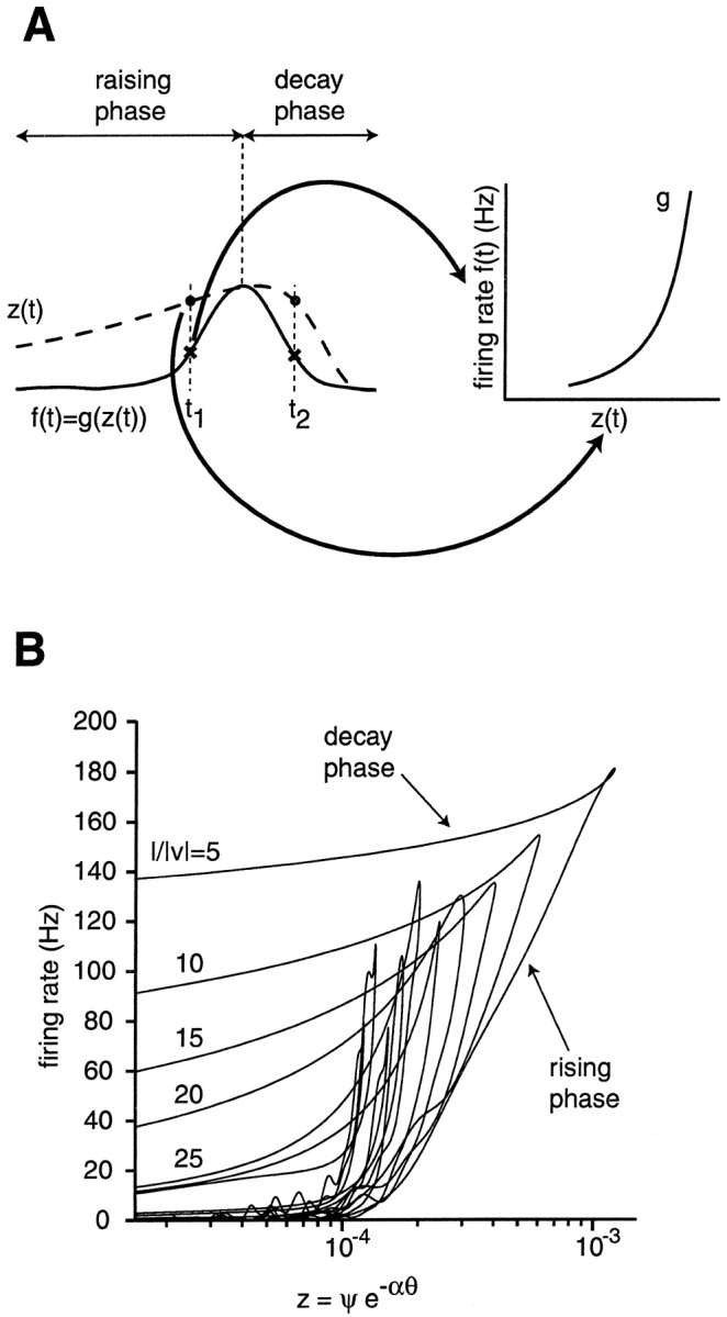
Determination of the static nonlinearity g from experimental data. A, The diagram on theleft illustrates the time course of the firing rate f(t) and of the kinematic variable z(t) during approach. Because f = g(z), one obtains g by disregarding the time parameter t and plotting for each t the pairs of values [z(t), f(t)] as illustrated on the right. According to Equation 11, g should be independent of l/‖v‖ and two time values t₁, t₂ on either side of the peak (rising and decay phase) for which z(t₁) = z(t₂) should yield f(t₁) = f(t₂).B, Static nonlinearity g obtained as inA for 10 values of l/‖v‖ (same experiment as in Figs. 2-4). The part of g corresponding to the rising phase is a steep nonlinearity well approximated by a saturating exponential (sigmoid function). For l/‖v‖ ≤ 25 msec, the firing rate f during the decay phase shows a hysteresis with larger values than during the rising phase.

Fig. 13.

Least square fits of g by the sigmoid function of Equation 4 (same preparation as in Fig.12B). A, Static nonlinearity g at four values of l/‖v‖ determined following the procedure outlined in Fig. 12A. For each panel thesolid line is the mean value of g , and thedotted line represents 1 SD from the mean. The dashed line is the best least square fit with the sigmoid function of Equation 4 (Materials and Methods). B, Fits of the time course of DCMD firing rate during object approach using Equation 11 and the function g determined in A. In each panel thesolid line is the time course of the firing rate during object approach (mean over 10 trials), the dotted line is the time course of the kinematic variable z(t) (see Eq. 12), and the dashed line is the fit with g, α, and δ determined as explained in Results. Note that in thebottom panel the fit is good up to the time point indicated by the arrow: for larger values of t, z(t) is identically equal to zero, and the time course of the firing rate falls outside the range of validity of Equation 11. A failure to fit the entire time course of LGMD and DCMD firing rate was observed in all of our 15 neurons at values of l/‖v‖ = 5 and 10 msec (see Discussion).

Table 4.

Numerical values of the parameters a,b, c, and x_1/2 (see Eq.4) characterizing the static nonlinearity g in four experiments (experiment 10797 is illustrated in Figs. 2-4, 11-13)

Experiment	b	l/‖v‖ = 50			l/‖v‖ = 40			l/‖v‖ = 30			l/‖v‖ = 20			l/‖v‖ = 10
		a	c	x1/2	a	c	x1/2	a	c	x1/2	a	c	x1/2	a	c	x1/2
10297	171		6.6	−9.0		4.6	−8.7		2.3	−8.2		3.1	−8.0		2.5	−7.6
		3	1.4	−8.3	2	1.8	−8.3	0	0.8	−7.3	8	1.5	−7.6	40	0.9	−7.0
10797	209		7.4	−8.9		7.6	−8.7		7.7	−8.5		4.7	−8.2		2.4	−7.8
		7	16.0	−9.0	8	12.0	−8.7	10	2.7	−8.7	15	0.8	−8.4	77	0.8	−7.6
10897	217		3.7	−9.3		4.7	−9.2		3.9	−8.9		3.8	−8.7		2.6	−8.2
		14	3.8	−9.6	8	4.6	−9.2	9	4.8	−9.0	10	1.8	−8.6	44	0.7	−8.1
12897	206		3.7	−9.4		3.7	−9.2		3.8	−9.0		3.0	−8.7		2.9	−8.3
		0	1.4	−9.1	3	2.0	−9.1	3	1.6	−8.9	7	1.4	−8.6	43	1.7	−8.3

For each experiment, the first line gives the parameters used in Equation 4 to fit g for the rising phase of the firing rate, and the second line gives the parameters used for the decay phase. Corresponding values of the slope and delay parameter for these experiments: α = 5.1; δ = 18 msec (10297); α = 4.7; δ = 27 msec (10797); α = 6.3; δ = 25 msec (10897); α = 6.3; δ = 28 msec (12897).

All the data analysis software was written using Matlab 5.0 and its graphical interface (The MathWorks, Natick, MA). The data of one experiment used in Figures 2-4, 7, and 12-14, as well as a Matlab M file generating Figure 3, are available on the World Wide Web (http://www. klab.caltech.edu/∼gabbiani/abstracts/Gabbiani_etal1998.html).

Fig. 7.

The time jitter in peak firing rate of LGMD and DCMD corresponds to a fixed angular error in the encoding of θ_thres. A, The two horizontal dotted lines show a fixed error (independent of l/‖v‖) in the encoding of θ_thres (indicated withcrosses) by the peak firing rate of LGMD and DCMD. This translates in the time domain to increasingly wide time windows Δt_thres for the jitter in peak firing rate as l/‖v‖ increases. The value of Δθ_thresdepicted in this example, 6.2°, corresponds to ±1 SD in Figure4A (i.e., Δθ_thres = 2 · ς_θthres according to the linear fit depicted inB below). B, The SD of the peak firing time shown in Figure 4A has been replotted as a function of l/‖v‖ and fitted with Equation 8. The correlation coefficient between l/‖v‖ and ς_tpeak is equal to 0.92, consistent with the prediction made by Equation 7. Corresponding angular error obtained from Equation 9: ς_θthres = 3.1°.

Fig. 14.

Dependence of g on l/‖v‖ (same preparation as in Figs. 12, 13).A, Value of the half-activation parameter x_1/2 and the slope a for 10 different values of l/‖v‖. The points taken from leftto right correspond to values of l/‖v‖ from 50 to 5 msec, respectively. Note the decrease in the slope parameter and the shift in half-activation as l/‖v‖ decreases. This is illustrated in the inset, which shows the 10 different sigmoids corresponding to the parameters shown in themain panel (a = 0; b = 209 Hz; see Eq.4). B, Hysteresis parameter as a function of l/‖v‖ (a is the asymptotic value of the firing rate as z becomes small; see Eq. 4).

RESULTS

The results presented here are based on recordings and complete analysis of the activity of 34 DCMD neurons in 34 different animals.

Peak response of DCMD and LGMD to simulated looming objects

The spontaneous activity of LGMD and DCMD was typically low (<1 Hz). LGMD and DCMD responded vigorously to the movement of small objects presented anywhere in the visual field of the stimulated eye and to simulated approach of looming objects on a collision course with the animal, as reported previously (Rowell, 1971a; Schlotterer, 1977;Pinter et al. 1982; Rind and Simmons, 1992). The response of LGMD and DCMD to looming objects was quite characteristic: it started early during the approach phase, usually before the object reached 10° in visual angle (Fig. 2). The firing rate gradually increased as the object grew larger, as if the cell were “tracking” the object over the approach. The firing rate then peaked and eventually decreased. On some occasions, the response was bimodal, with a brief interruption of spiking during object approach (Fig. 2, arrow), as reported by others (Schlotterer, 1977;Pinter et al., 1982). During the course of an experiment (which usually lasted between 1 h 15 min and 1 h 30 min and in which trials with different values of l/‖v‖ were interleaved pseudo-randomly; see Materials and Methods), the response to repeated presentations of the same stimulus was quite variable from trial to trial. In some of the neurons studied, part of this variability was attributable to habituation of the response to the stimulus, as illustrated in Figure 3, left panels (see in particular the trials for l/‖v‖ = 50, 45, and 35 msec). This habituation was reflected by the high SD in the number of spikes elicited per trial, relative to the mean. Clear effects of habituation could be seen by visual inspection of the raster plots in 2 of 15 cells studied. Even when the SD in the number of spikes elicited was low (as illustrated in Fig. 3, right panels), repeated presentations were characterized by a substantial jitter in the spike occurrence times.

To study the time-course of the firing rate of DCMD and LGMD during object approach, each individual spike raster was convolved with a 20 msec Gaussian window to obtain an estimate of the instantaneous firing frequency and its SD (Figs. 2, 3, solid and dotted lines; also see Materials and Methods). Visual inspection of the instantaneous firing rate as a function of l/‖v‖ revealed that the peak in DCMD firing rate consistently shifted toward collision as l/‖v‖ decreased (Fig. 3, read fromtop to bottom and from left toright) to eventually occur at, or even after, predicted collision for small values of l/‖v‖ (corresponding to small and/or fast-moving objects). This observation could also be made directly from inspection of the instantaneous frequency plots computed from single trials (see Fig. 2) and was independent of the variability described in the previous paragraph.

A plot of the time of peak firing, ‖t_peak‖, versus l/‖v‖ revealed that these two variables were linearly related (Fig.4A): correlation coefficients between ‖t_peak‖ and l/‖v‖ ranged from 0.98 to 1.0 (mean ± SD, 0.99 ± 0.01; N = 15 neurons). Similar results were observed for all 34 neurons building our database. We therefore performed, for each experiment, a linear regression of the peak time versus l/‖v‖,

$$‖t_{\text{peak}}‖=\alpha \frac{l}{\Vert v\Vert }-\delta ,$$ Equation 5

and estimated the slope (called α) and the intercept (called δ) characterizing these linear fits (Fig. 4A, inset) as well as the errors in the estimates of α and δ. Note that although α is dimensionless, δ is in units of time. This analysis revealed that the estimates of α and δ were not independent of each other, as might be expected a priori, but rather were tightly correlated (range of observed correlation coefficients, 0.73–0.96; mean ± SD, 0.85 ± 0.09; N = 15 neurons). In other words, a higher (lower) value of α is more likely to coincide with a higher (lower) value of δ, respectively. This is illustrated in Figure 4B, where the 68.3% confidence region for the values of α and δ are depicted. The tilted ellipsoidal shape of the confidence region reflects the correlation between the estimates of the two variables (uncorrelated estimates would yield ellipses with principal axes parallel to the x- and y -coordinate axes).

Significance of the linear relation between peak firing time andl/‖v‖

The significance of the experimentally determined linear relation between the peak DCMD firing rate relative to collision and the parameter l/‖v‖ as well as the correlation between the estimates of α and δ can be explained by the following observation.

For a given DCMD neuron, let α be the slope and δ the intercept of the linear regression between peak time and l/‖v‖ (see Fig. 4A, Eq. 5). Consider the angular size, call it θ_thres, subtended by the approaching object δ msec before the peak (see Fig. 1A for the definition of θ). Equation 5 states that this angular size is independent of l/‖v‖, i.e., independent of the particular size or speed of the approaching object. To see this, note that by trigonometry,

$$tan\frac{{\theta }_{\text{thres}}}{2}=\frac{l}{x(t_{\text{peak}}-\delta )}\hspace{1em}(\text{using Eq}.2),$$

$$=\frac{l}{v·(t_{\text{peak}}-\delta )}\hspace{1em}(\text{using Eq}.1),$$

$$=\frac{l}{\Vert v\Vert ·\left(\alpha \frac{l}{\Vert v\Vert }\right)}$$

$$=\frac{1}{\alpha }\hspace{1em}(\text{using Eq}.5;\text{see Appendix} 1).$$

Furthermore, this calculation shows that the angular threshold size characterizing the peak response of a given DCMD neuron (to occur δ msec later) is completely determined by the slope of the linear regression line as:

$${\theta }_{\text{thres}}=2·{tan}^{-1} \frac{1}{\alpha }.$$ Equation 6

For the DCMD neuron depicted in Figures 2-4, this means that the peak firing rate always occurred 27 msec (±3 msec) after that the object had reached a full angular size (θ_thres) of 24° (±1.5°) on the locust’s retina, for all values of l/‖v‖, as illustrated in Figure 5.

Fig. 5.

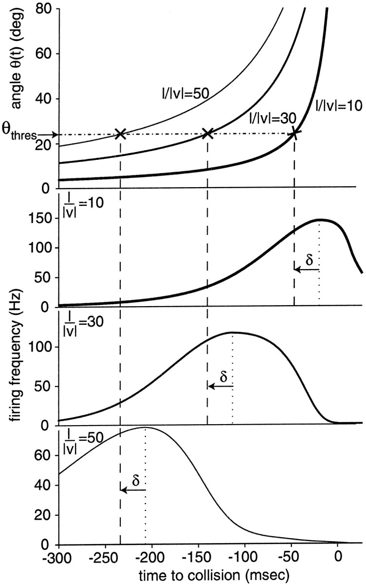
Diagram illustrating the significance of Equation5 for the time course of the DCMD response to looming objects.Top panel, Angle of an approaching square for three different values of l/‖v‖ (10, 30, and 50 msec; Eq. 2).Bottom three panels, Time course of DCMD firing rate in response to these stimuli. The time of peak firing follows the same linear relation (Eq. 5) observed in Figs. 3 and 4. In each case, the time of peak firing is indicated by the dotted vertical lines. The three vertical dashed lines are placed δ = 27 msec before the peak. At this moment the angle subtended by the object is θ(t) = 24° for all three experiments. [Eachvertical dashed line intersects its angular size stimulus curve (×) at a constant y = θ_thres = 24°.]

Equation 6 also offers a simple explanation for the experimental correlation observed between the parameter α and δ characterizing the linear relation between the peak time and l/‖v‖ (Fig. 4B). If the threshold angle θ_thres is overestimated (corresponding to an underestimation of α, according to Eq. 6), then we expect to underestimate the delay between the angular threshold size and the time of the peak firing rate. Conversely, if the angular threshold size is estimated as being smaller than its real value, we should overestimate the time interval separating the instant when the object reaches the threshold angle and the peak firing rate.

Estimates of the slope, delay, and angular threshold size are plotted for 15 animals in Figure 6. The values of these parameters varied from animal to animal but were consistently found to range between 15 and 35 msec delays for angular threshold sizes between 15 and 40°. Part of this variability might arise from interindividual differences in the geometric characteristics and size of the eye.

Accuracy of the angular threshold computation

If the angular threshold computation implemented by LGMD and DCMD is performed with a fixed angular accuracy, Δθ_thres, one expects the variability in peak occurrence time, Δt_thres, to increase with l/‖v‖. This point is illustrated in Figure7A. The dotted horizontal lines represent a constant error Δθ_thres for the angular threshold size θ_thres. In the time domain, this constant error translates into increasingly large tolerance windows Δt_thres for the peak occurrence time (delimited by pairs of dotted vertical lines) because as l/‖v‖ increases, the rate of angular change (dθ/dt) decreases at the threshold angle θ_thres (see Fig. 7A, Eq. EA8 in Appendix).

As derived in Appendix , the accuracy of peak timing is predicted (to first order) to increase linearly with l/‖v‖ for Δθ_thres fixed,

$$\mathrm{\Delta }{t}_{\text{thres}}=\frac{1}{2} (1+{\alpha }^2)·\mathrm{\Delta }{\theta }_{\text{thres}}·\frac{l}{\Vert v\Vert },$$ Equation 7

where α is the slope of the regression line defined by Equation5. The SD, ς_tpeak, of ‖t_peak‖ characterizes the accuracy of peak timing. To assess the validity of Equation 7, we therefore performed a linear regression of ς_tpeak as a function of l/‖v‖,

$${\varsigma }_{{\text{t}}_{\text{peak}}}=\rho \frac{l}{\Vert v\Vert },$$ Equation 8

(Fig. 7B). Correlation coefficients between ς_tpeak and l/‖v‖ ranged from 0.56 to 1.0 (mean ± SD, 0.87 ± 0.15; N = 15 neurons), consistent with this linear assumption.

Next we tested whether the peak time in DCMD response and its variability could be described by a simple model depending only on three free parameters: (1) the threshold angle θ_thresencoded by the peak firing rate of LGMD and DCMD; (2) the delay δ between the angular threshold size and peak time; and (3) the accuracy ς_θthres with which the threshold angle is encoded by a given neuron. The first two parameters can be obtained from the experimental data by linear regression of peak time versus l/‖v‖ (see Eqs. 5 and 6), whereas ς_θthres can be obtained by combining Equations 7and 8,

$${\varsigma }_{{\theta }_{\text{thres}}}=\frac{2\rho }{(1+{\alpha }^2)},$$ Equation 9

where ρ is the slope of the linear regression between ς_tpeak and l/‖v‖ (seeBevington and Robinson, 1992, Sec 3.2).

Ten of 15 neurons tested had a distribution of peak firing times as a function of l/‖v‖ in close agreement with the model (see Materials and Methods; χ²/F range, 0.19–4.1; mean ± SD, 1.88 ± 1.52; F statistics range, p ≥ 0.05–0.96; mean ± SD, 0.38 ± 0.29; K.–S. test range, p ≥ 0.01–0.96; mean ± SD, 0.58 ± 0.32). No neuron failed to pass more than one of these three tests: two neurons had high values of χ²/F (5.0 and 11.5, respectively); one failed to pass the F test (p < 0.05); and the remaining two failed the K.–S. test (p < 0.01). In three of these five cases, failure was attributable to a small number of outliers (one to three) among the 50 test peak time values, causing a significant distorsion in the distribution of fit residuals. The remaining two cases appeared to represent genuine failure of the model to represent the data. For the 10 neurons best described by the model we also verified that the experimental values of α and δ, their SDs, and correlation coefficient could be reproduced by the model. To this end, we generated synthetic data sets consisting of 100 peak times and recomputed these parameters. For the neuron depicted in Figures 4 and 7B, for example, 25 synthetic sets yielded a range of values (α = 4.47–4.77; SD = 0.18–0.30; δ = 24.1–28.7 msec; SD = 1.7–4.5 msec; correlation coefficient = 0.71–0.79) in close agreement with the experimental ones (α = 4.68 ± 0.29; δ = 27 ± 3.2 msec; correlation coefficient = 0.76).

Among the 10 neurons that successfully passed all three criteria described above, the angular errors computed using Equation 9 ranged from 3.1 to 11.9°. These angular errors correspond to the angle defined by two to six ommatidia on each side of the expanding object.

Test of possible artifacts attributable to video refresh

Because images of approaching objects were updated every 5 msec on the monitor screen (200 Hz refresh; see Materials and Methods), the resulting visual stimulation was only an approximation of the continuous motion of real objects. A possible artifact caused by such discontinuous image updates would be a progressive failure to stimulate the neuronal motion circuitry presynaptic to LGMD when the jump in image size exceeds 3° (i.e., twice the locust’s photoreceptor acceptance angle; Osorio, 1986b). In this case, the early decrease in DCMD activity could be attributable to a lack of appropriate stimulation after the time at which angular increments exceed 3° (Rind and Bramwell, 1996, note added in proof; Rind and Simmons, 1997;Judge and Rind, 1997). It is therefore important to rule out the possibility of such a stimulation artifact. The following two observations show that no such artifact occurred in our experiments.

First, for large objects or low velocities of approach (l/‖v‖ ≥ 25 msec) the peak firing rate occurred well before the angular increment reached 3°. This is illustrated in Figure 2 for one experiment (l/‖v‖ = 45 msec) in which only the last image update, 112 msec after the peak firing rate, led to an angular increment >3°, and in Table 2for 15 other experiments (l/‖v‖ = 25 msec). The average angular step at threshold was 0.60 ± 0.33°, ranging from 0.2 to 1.2° (Table 2). Second, assuming an artifact caused by stimulation failure is equivalent to stating that the peak in DCMD firing rate should be correlated with an angular velocity threshold ψ_thres = 600°/sec (3°/refresh × 1 refresh/5 msec) rather than an angular size threshold θ_thres (between 15 and 40°), as reported here. By setting ψ_thres = 600°/sec and solving for ‖t_peak‖ as a function of l/‖v‖ in Equation 3 (see Appendix ), one obtains a relation between peak time and l/‖v‖ that is plotted in Figure 8A (dashed line), together with the experimental results of one DCMD experiment. As can be seen, the relation between peak time and l/‖v‖ predicted by an angular velocity threshold model (Fig. 8A, dashed line) provides a very poor fit of the data compared with the excellent fit obtained with Equation 5(Fig. 8A, solid line). For low values of l/‖v‖, for example, large angular jumps occur soon during the stimulation, and the peak time is predicted by the angular velocity threshold model to actually occur earlier than observed experimentally. This prediction could be confirmed in none of N = 9 animals specifically tested for this using a protocol containing five values of l/‖v‖ < 10 msec (Fig. 8A; variant of first protocol, see Materials and Methods). Introducing a constant delay between the curve ψ_thres = 600°/sec and the peak time produced a better fit of the experimental data for l/‖v‖ ≅ 5 msec but much poorer fits for all other values of l/‖v‖ (Fig.8A, dotted line).

Table 2.

At peak time, angular jump sizes are well below 3° for l/‖v‖ ≥ 25 msec

Experiment	Threshold angle θthres(°)	Delay δ (msec)	Jump at threshold (°)	Jump at peak time (°)
81197	34.6	17.8	1.1	1.8
81297	37.0	16.9	1.2	1.8
81397	19.4	30.2	0.3	0.5
81597	19.4	28.1	0.3	0.5
82097	21.0	23.1	0.4	0.6
82697	35.6	23.6	1.1	2.1
92497	28.4	31.8	0.7	1.4
92997	30.6	15.0	0.9	1.2
93097	25.2	25.7	0.5	0.9
10297	22.4	18.4	0.5	0.6
10397	15.8	26.3	0.2	0.3
10697	28.4	17.0	0.7	1.0
10797	24.2	27.0	0.5	0.9
10897	18.0	25.4	0.3	0.4
12897	18.0	28.1	0.3	0.4

The first three columns report the threshold angle θ_thres as well as the delay δ obtained according to Equations 5 and 6 for 15 different DCMD neurons for l/‖v‖ = 25 msec (see Results and Fig. 5). The fourth column reports the value of the angular jump in image size δ msec before the peak (i.e., at t_peak − δ; see Fig. 5), whereas the last column is the angular jump at peak time. All angular jump values are well below 3°.

Fig. 8.

No indication of angular velocity threshold artifacts was seen both at high and at low image refresh rates with the video stimulation system used in the present experiments. A, The experimental dependence of peak firing time as a function of l/‖v‖ (filled dots, mean ± SD) is well fitted by the linear relationship corresponding to an angular threshold θ_thres = 26° and a delay δ = 27 msec between the time of threshold angle and peak time (solid line a; see Eq. 5). In contrast, the prediction that the peak time should occur immediately after an angular jump of 3° in the image (dashed line b) only poorly fits the data. The same is true when a fixed delay is inserted between the time of 3° image jump and the peak, thus shifting the curve downward (dotted line c; same delay δ = 27 msec as for the angular threshold line θ_thres = 26°). See Appendix for the derivation of the angular threshold curve (Eq. EA7). B, Dependence of peak time as a function of l/‖v‖ for three different refresh rates of the video monitor (squares, 200 Hz; circles, 100 Hz; triangles, 67 Hz). The best linear fits to Equation5 (dotted line, short dashed line, long dashed line, respectively) virtually overlap in all three cases. For the sake of clarity only the largest SD of the mean peak time estimate in one direction is shown at each value of l/‖v‖ . Data in A and B are from two different experiments.

Because our earlier experiments were performed with a refresh rate of 1/13.9 msec (72 Hz; Hatsopoulos et al., 1995), we also verified that low refresh rates did not affect the validity of our results. To this end, we used three different refresh rates (pseudorandomly interleaved trials) in five animals (200, 100, and 67 Hz; second protocol, Materials and Methods). The results of one such experiment and the best linear fits to the data are plotted in Figure 8B. No significant change in the time of peak firing rate as a function of l/‖v‖ was observed in three of five experiments. In one preparation, lower refresh rates led to slightly earlier peak times. In the fifth preparation, lower refresh led to slightly later peak times (Table 3). In accordance with these results, and in contrast to those reported by Rind and Simmons (1997), little or no phase locking of the DCMD response to the image refresh could be observed at 67 or 200 Hz. This could be seen from the spike rasters obtained in response to individual trials, as illustrated in Figure 9 (compare with Rind and Simmons, 1997, their Fig. 4). Rind and Simmons (1997) also reported that a failure to properly stimulate DCMD results in a significant decrease in the number of action potentials elicited by a stimulus. We therefore compared the number of action potentials elicited at 200 Hz (n₂₀₀) to that obtained at 67 Hz (n₆₇). The mean difference, 〈n₂₀₀ − n₆₇〉 = 0.74 ± 6.1 action potentials, was not significantly different from zero (mean ± SD averaged over five experiments and eight protocols). DCMD was therefore equally well excited by stimuli presented at 67, 100, and 200 Hz, and none of the artefacts reported byRind and Simmons (1997) could be observed in the present experiments.

Table 3.

Lower refresh rates do not lead to consistent changes in peak firing time as a function of l/‖v‖

Experiment	200 Hz		67 Hz		Difference
	Slope α (mean ± SD)	Delay δ (msec) (mean ± SD)	Slope α (mean ± SD)	Delay δ (msec) (mean ± SD)
12997	6.1  ± 0.5	28.4  ± 3.1	5.6  ± 0.2	27.8  ± 1.6	No
12997a	4.1  ± 0.7	14.5  ± 6.5	4.7  ± 0.6	21.0  ± 6.5	No
121097	6.5  ± 0.6	43.2  ± 5.0	6.6  ± 0.5	47.8  ± 3.8	No
121197	3.0  ± 1.0	24.0  ± 10.8	5.4  ± 0.4	44.3  ± 3.8	↑
121197a	5.7  ± 0.7	30.6  ± 6.5	4.1  ± 0.4	17.7  ± 2.8	↓

Parameters α and δ of Equation 5 are reported for five experiments at two refresh rates (200 and 67 Hz). Data points and straight line fits are shown in Figure 8B for experiment 121097. The last column indicates whether differences were observed between the values of α and δ at 200 and 67 Hz. No, SDs of both parameters measured at 67 and 200 Hz overlapped. Downward arrow, Decrease in peak time ‖t_peak‖ at lower refresh. Upward arrow, Increase in peak time at lower refresh.

Fig. 9.

No phase locking of the DCMD response could be observed at either 200 or 67 Hz refresh. Top panel, Half-angle of the object presented on the screen as a function of time for a value of l/‖v‖ = 5 msec and a refresh rate of 200 Hz (angular image increments are determined by differences in successive values of θ/2). The five rasters below show the DCMD response to this stimulus (the dotted lines are placed 5 msec apart and aligned with the time of image refresh). The next five rasters report the response of the same DCMD neuron to the same stimulus but with the monitor image refreshed only every 15 msec (67 Hz), as illustrated in the bottom panel (thedotted lines are placed 15 msec apart and aligned with the time of image refresh).

Effect of background luminance and stimulus contrast on peak firing time

Next, we investigated whether the mean light level input to photoreceptors or the contrast of the edges of the object sweeping across the receptive field during visual stimulation affected the timing of the peak response and/or its relation to the angular threshold size characteristic of a given DCMD neuron. To this end, a series of experiments was performed where the relative background luminance, B, and object luminance, O, were systematically varied. Data was collected at three values of l/‖v‖ (third protocol, Materials and Methods). These three values were selected among those used in the previous two protocols to yield the most reliable estimates of the slope and delay parameters (α and δ, respectively; see Eq. 5). In this way, a large range of background and contrast combinations could be explored in a single DCMD neuron while retaining the ability to detect possible deviations from linearity in the peak time versus l/‖v‖ relation as well as possible changes in α and/or δ. As illustrated in Figure 10, A andB, in one experiment, the linear relation between peak time relative to collision and l/‖v‖ remained valid for a wide range of background and contrast values. This result and the following ones were observed in all neurons tested (N = 6). No statistically significant changes in the angular threshold size (θ_thres) or the delay (δ) were observed for decreases in background luminance up to one-fourth of the maximal value (Fig. 10A). Similarly, the number of action potentials elicited per trial did not change in a statistically significant way as the background luminance decreased (see one example in Fig. 10B). Note that for the experimental results depicted in Figure 10, B and D, there was a statistically significant decrease in the number of action potentials elicited at l/‖v‖ = 40 msec (≅35 per trial) compared with l/‖v‖ = 10 msec (≅20 per trial). This observation could be made in only two of six preparations (the experiment illustrated in Fig. 3, for example, showed no significant decrease in the number of action potentials with l/‖v‖). On the other hand, the number of action potentials elicited per trial was always significantly dependent on the contrast of the edge of the stimulus in the range tested (from −1.00 to −0.25), as illustrated in one example in Figure 10D. To characterize this dependence, we pooled for each experiment data obtained at different background luminances and performed a linear regression of the mean number of action potentials elicited as a function of contrast separately for each value of l/‖v‖. The slope of these regression lines ranged from −6.3 ± 2.6 to −35.3 ± 4.7 spikes/unit of contrast and was significantly correlated with l/‖v‖ in four of six cases (larger values of l/‖v‖ leading to larger drops in the number of action potentials elicited per trial as contrast varied from −1.00 to −0.25). Remarkably, this decrease in mean stimulus-evoked activity affected neither the timing of the peak nor the values of the angular threshold size and delay (Fig. 10C). No statistically significant increase in the SD of peak time estimates could be observed. Therefore, in the present experiments the angular threshold computation characterizing the response of DCMD to looming stimuli remained valid over a wide range of background luminances and contrasts.

Fig. 10.

The linear relation between l/‖v‖ and peak firing time is independent of background luminance or stimulus contrast, despite decreased responses at lower contrasts. A, Peak firing time relative to collision as a function of l/‖v‖ for four background luminances (B = 100%; 75, 50, and 25% of I_max = 95 cd/m²). Dashed line, Best linear fit for B = 75% (α = 4.20 ± 0.34; δ = 11.9 ± 6.6 msec). For clarity, only one linear fit is shown, and only the largest error for each value of l/‖v‖ is illustrated in one direction. B, Mean number of spikes ±SD elicited per trial for the same four background luminances as in A(symbols as in A). C, Peak firing time as a function of l/‖v‖ at four contrasts (C = −1.00, −0.75, −0.50, and −0.25). Dashed line, Best linear fit for C = −0.25 (α = 4.47 ± 1.56; δ = 17.9 ± 16.6 msec). D, Mean number of spikes ± SD elicited per trial for the same four contrasts as in C (symbols as in C). Data in A–D are from a single experiment.

Effect of body temperature on peak firing time

Because locusts exert only a limited control over their body temperature, it is expected to fluctuate over a large range of values depending on external conditions and on metabolic rate. In particular, in flying insects, body temperature is known to rise significantly during intense periods of muscular activity such as flight episodes (Weis-Fogh, 1956, 1964; Neville and Weis-Fogh, 1963; Stavenga et al., 1993). We studied the effect of body temperature on the timing of peak firing rate, the angular threshold, and delay parameters by comparing the responses to looming stimuli elicited at room temperature (21–24°C) with those obtained at 30–33°C (fourth protocol, Materials and Methods). In all neurons tested (N = 8), raising body temperature resulted in a significant shortening of DCMD action potentials (see example in Fig.11, top inset; mean decrease, 35.5 ± 4.5%, measured in N = 4 animals with best recording signal-to-noise ratio) but no consistent changes in the number of action potential elicited during each trial was observed. The timing of the peak response was also unaffected (N = 8 neurons), as illustrated in Figure 11. In this experiment, the response to looming stimuli was recorded successively at room temperature (21°C, squares), 30°C (circles), and back at room temperature (triangles). The values of the parameters α and δ obtained by fitting straight lines to the data were accordingly not significantly affected by temperature (Fig. 11,bottom inset). Therefore, our characterization of the DCMD response remained valid over a 12°C range of ecologically relevant temperatures.

Fig. 11.

Effects of body temperature on the DCMD response to looming stimuli. Top inset, Two extracellular action potentials recorded at room temperature (21°C, trace i) and at 30°C (trace ii). Note the significant decrease (43%) in the width of trace ii compared with i (measured as the time difference between the arrows shown on the inset). Main panel, Time of peak firing relative to collision as a function of l/‖v‖ at room temperature (squares), 30°C (circles), and during a subsequent control experiment back at room temperature (triangles). For clarity, only the largest error bar is shown at each value of l/‖v‖. Note the increased variability in the peak response compared with Figure 7 or 9, for example. This was presumably because of the longer time span of the experiment (2 h 30 min in this case) caused by heating and cooling of the animal. Solid lines, Best linear fits to the data using Equation 5. Bottom inset, Values of the parameters α and δ for each of the three fits ± SD showing no significant differences in the mean values. Data are from a single experiment.

Time course of firing rate as a function of retinal object size and edge angular velocity

We next studied the dependence of the angular threshold computation implemented by LGMD and its presynaptic circuitry on the physical variables characterizing object approach. Two such kinematic variables that can be measured at the retina are the angular size and edge velocity (see Fig. 1). We therefore looked for a class of functions f of these variables that could describe the time course of LGMD and DCMD firing rate over the range of values of l/‖v‖ used in the present experiments (see Fig. 3). Remarkably, only three assumptions derived from experimental data tightly constrain the functional dependence of the firing rate on angular size and velocity of approach, as we now explain.

From earlier anatomical and electrophysiological characterizations of LGMD responses (Palka, 1967; O’Shea and Rowell, 1976; Rowell et al., 1977) and from the results presented here, it is plausible that the class of functions f describing the firing rate of LGMD and DCMD neurons should satisfy the following three assumptions:

(1) f should depend only on the angular size, θ(t), and angular edge velocity, ψ(t), of the approaching object. These two variables are thought to be represented in the form of inhibitory (size-dependent) and excitatory (motion-dependent) inputs to the various dendritic subfields of LGMD (Palka, 1967; O’Shea and Rowell, 1976; Rowell et al., 1977; also see Discussion). Another kinematic variable of the approach that might play a role in describing the firing rate of LGMD and DCMD (Rind and Simmons 1990, 1992), the angular acceleration of the object, was ruled out as sole explaining parameter in an earlier series of experiments (Hatsopoulos et al., 1995).

(2) The firing rate at time t depends only on the value of θ and ψ at time t − δ. In other words, if we set x(t) = θ(t) and y(t) = αψ(t) , then:

$$f(t)=f(x(t-\delta ),y(t-\delta ))$$ Equation 10

(see Eq. 5 for the definition of α and δ). A delay between firing rate and stimulus is expected because of the lags introduced by synaptic and cellular elements along the neuronal pathways converging onto LGMD. Here, this delay is δ, the delay observed between the peak response and the threshold angle preceding it (Fig. 5).

(3) The peak of f(t) should satisfy the linear relation observed experimentally between peak firing rate time and l/‖v‖ (see Figs. 4, 10, 11), regardless of the particular values of θ_thres and δ implemented by the LGMD neuron of a given animal. In other words, we seek to characterize a class of functions that can take into account the different angular threshold sizes and delays (see Fig. 6) as well as the variability in the time course of the firing rate observed across animals (data not shown, but see Table 4).

As derived in Appendix , it follows from assumptions 1–3 above that f has to be of the form,

$$f(t)=g(\psi (t-\delta )·e^{-\alpha \theta (t-\delta )}),$$ Equation 11

where g is a static nonlinearity that characterizes the transformation between the kinematic variable z = ψ · e^−αθ and the firing rate (see next section; Fig.12A).

Thus each function belonging to the class given in Equation 11 depends on three parameters: α, δ, and the static nonlinearity g. To understand why this class of functions can describe the time course of LGMD firing rate during object approach, note that because g is a static (time-independent) function, the time course of the firing rate is entirely determined by:

$$z(t)=\psi (t-\delta )·e^{-\alpha \theta (t-\delta )}$$ Equation 12

$$=\psi (t-\delta )/e^{\alpha \theta (t-\delta )}.$$

Both ψ and θ are nonlinear increasing functions of time during the approach (Eqs. 2, 3; Fig. 1B). The combination of ψ and θ in Equation 12 is such that ψ acts as an excitatory term (an increase in ψ leads to an increase in z and thus in the firing rate), whereas θ acts as an inhibitory term (an increase in θ leads to an increase in e^αθand thus a decrease in z and in firing rate; see Eq. 12). Therefore, the apparent excitatory and inhibitory effect of motion and size (respectively) on the LGMD response (Palka, 1967; O’Shea and Rowell, 1976; Rowell et al., 1977) can be predicted on the basis of assumptions 1–3 alone under our experimental conditions. At the onset of approach, the motion-dependent excitation represented by ψ increases faster than e^αθ, leading to an increase in firing rate. Some time later, size-dependent inhibition gains importance because of its exponential dependence on θ. It eventually overcomes the excitatory term, leading to a decrease in the response. The time at which inhibition overcomes excitation always occurs a fixed delay δ after that the object has reached an angular threshold 2 · tan⁻¹1/α, independent of l/‖v‖ (Eq. 12), as observed experimentally. In addition, under assumptions 1–3 above, this is the only functional combination of ψ and θ with this property.

Experimental determination of the static nonlinearity g

It follows from Equation 11 that the static nonlinearity g characterizes the transformation between the kinematic variable z = ψ · e^−αθand the firing rate during approach (Fig. 12A,left). To determine the function g(z) that best fits the experimental data, the values of α and δ were first obtained for each DCMD neuron by a linear fit of the peak firing time relative to collision versus l/‖v‖, as explained earlier (Fig. 4, Eq. 5). We then computed z(t) as a function of time during object approach (see Eq. 12) and plotted for each value of t the experimental value of the firing rate versus z (nonparametric plot; Fig. 12A,right). This procedure was repeated for each value of l/‖v‖ tested experimentally. The dependence of g on z obtained for 10 different values of l/‖v‖ for a single DCMD neuron (first protocol, Materials and Methods) is shown in Figure 12B (note the logarithmic scale of the horizontal axis in this figure and in Figs. 13A,14A,inset). In contrast to the prediction of Equation 8, g was not independent of l/‖v‖ (see Discussion): the dependence of g on z was typically steeper for large values of l/‖v‖. The function g also exhibited hysteresis at small values of l/‖v‖ (≤20 msec). This meant that, for a fixed value of z, the firing rate was typically higher after than before the peak (Fig. 12A, B), reflecting a slower “shutdown” than “buildup” of excitation during object approach.

To characterize quantitatively these two observations, we fitted separately the parts of g corresponding to the rising and falling phase of the firing rate at each value of l/‖v‖ with a sigmoid function (see Eq. 4, Materials and Methods; Table 4). This led to satisfactory fits of g and of the time course of the firing rate during approach in 13 of 15 neurons (Fig.13A, B). The parameters x_1/2 (half-activation) and c (slope) characterizing g for the rising phase of the firing rate (Eq. 4) were positively and negatively correlated with l/‖v‖ (Fig. 14A), reflecting the shift in the dependence of g on z with l/‖v‖ and its shallower slope (Fig.14A, inset), respectively. The dependence of the parameter a characterizing hysteresis as a function of l/‖v‖ for the neuron of Figure 12Bis illustrated in Figure 14B.

DISCUSSION

This series of experiments and theoretical analysis were aimed at characterizing the computation performed by LGMD and DCMD in response to objects approaching on a collision course with the animal. Because the peak firing rate always occurred a fixed delay after the object had reached a constant angular size on the animal’s retina, this suggests that LGMD computes the time at which this threshold angle is reached during object approach. For each animal, θ_thres is constant over one order of magnitude of the kinematic approach parameter l/‖v‖. The algorithm underlying this computation requires a multiplication of two nonlinear functions of time that characterize the stimulus projection on the retina: these functions are the angular size, θ(t), and the angular velocity, ψ(t), of the approaching object.

The visual stimulus

In these experiments, the locust’s visual system was stimulated with a monitor screen refreshed at 200 Hz. This allowed for a good control of the stimulus time course but represented only an approximation of true motion. Several arguments rule out the possibility of stimulation artifacts.

First, the temporal cutoff frequency of locust photoreceptors is less than half the monitor refresh rate, ruling out a locking of the photoreceptor response to video refresh (Miall, 1978; Howard, 1981;Howard et al., 1984). Osorio (1986b) reported a decrease in the response of medullary motion-detecting neurons for temporally offset flashes spaced more than 3° apart. His results do not apply to our experimental situation, because all photoreceptors on the looming motion trajectory were stimulated.

Second, a stimulation artifact predicts that the peak firing rate should follow a very different relation with l/‖v‖ than that observed experimentally. Because our earlier experiments (Hatsopoulos et al., 1995) were performed at a lower refresh rate (72 Hz) we verified that none of our results depended on refresh rate and that DCMD was equally well stimulated at lower refresh frequencies. Thus, the statement that “The peak in DCMD activity measured byHatsopoulos et al. (1995) occurred when the jump size on the monitor first exceeded approximately 3°” (Judge and Rind, 1997, p 2210) is incorrect (Fig. 2, Table 2) and the statement that the “DCMD response reported by Hatsopoulos et al. (1995) is an artifact” (Rind and Simmons, 1997, p 1032) (also see Rind and Bramwell, 1996, note added in proof) is erroneous.

Finally, the occurrence of peak DCMD activity before collision at high values of l/‖v‖, as observed here, is supported by earlier reports (Schlotterer, 1977, their Fig. 3; Pinter et al., 1982, their Figs. 1A, 2A(i)), including Rind and Simmons’ own recordings (Rind and Simmons, 1992, their Fig. 4). As demonstrated here, however, the timing of the peak depends on l/‖v‖. Therefore, if sufficiently small values of l/‖v‖ are selected, a substantial portion of the spikes, including the peak, will occur after collision (for example, see Fig. 3, l/‖v‖ = 5 msec; also see Judge and Rind, 1997, their Fig. 4, top, which corresponds to l/‖v‖ = 6 msec).

Behavioral relevance of the angular threshold computation

Peak DCMD activity always occurred a fixed time after that the size of the object reached an angular threshold. This information might thus be used by the animal to initiate an escape behavior in face of an imminent danger. In our earlier experiments (Hatsopoulos et al., 1995, note 15), the time of peak DCMD activity was correlated with the subsequent timing of a femoro-tibial flexion for presumed jump preparation (for a similar observation, also see Wallace, 1958; Wehner, 1981, p 479). This flexion occurred a fixed delay (20 msec) after the peak, and after that the object had reached a fixed angular threshold size on the retina. Robertson and Johnson (1993a,b) recently characterized the cues used by locusts in visually triggered collision avoidance maneuvers during flight. They concluded that the variable most closely related with the avoidance maneuver was the angular size of the object 65 msec before its initiation. The threshold angles reported by them, 10° (Robertson and Johnson 1993a, their Fig. 3, b, their Table 2), are smaller than the typical threshold angles reported here. Because in their study, objects approached on a frontal rather than side collision course, this difference might be related to the better acuity in the frontal visual field (Horridge, 1978).

These two lines of evidence as well as anatomical cues suggest that LGMD and DCMD are part of a fast neuronal pathway initiating escape responses. In pigeons, neurons with response properties very similar to those described here have been recently reported in nucleus rotundus, the homolog of the mammalian inferior caudal pulvinar (Sun and Frost, 1998). Interestingly, this nucleus also contains neurons sensitive to angular velocity and others yet sensitive to time to contact. The nucleus rotundus is thought to play a important role in the “tracking” of approaching objects. Clearly, angular threshold size has disadvantages when compared with time to contact (Lee and Reddish, 1981; Wagner, 1982; Wang and Frost, 1992): given a fixed angular threshold size, the timing of the response will occur later for objects moving faster. However, this might prove sufficient for a restricted range of object sizes and velocities as encountered in natural environments (Robertson and Johnson, 1993a,b). In this context, it is also important to assess the dependence of this computation on the nature of the looming stimuli. Our results demonstrate stability over a wide range of backgrounds and contrasts despite a decrease in spike rate with contrast (for a similar dependence of spike activity on contrast, see Palka and Pinter, 1975; Judge and Rind, 1997). Similarly, we showed invariance to physiological body temperature changes.

Whether the peak activity or some physiologically related variable is extracted by the motor circuitry postsynaptic to DCMD remains an open question. Formally, peak detection is equivalent to the detection of a zero crossing in the time derivative of the firing rate, a problem extensively investigated in mammalian vision (Marr, 1982). Alternatively, it is possible that an integration mechanism similar to the one proposed for the triggering of the landing response in flies (Borst and Bahde, 1988; also see Sun and Frost, 1998, their Fig. 3a) might underlie the processing of DCMD firing rate by postsynaptic neurons. Isolating this mechanism is complicated by the divergent connections made by DCMD and by the existence of >10 lobula neurons with response properties similar to DCMDs (Gewecke and Hou, 1993).

Representation and algorithm

We have shown that a particular combination of the object angular size θ(t) and of its angular edge velocity ψ(t) can describe phenomenologically the time dependence of the peak firing rate on l/‖v‖. Furthermore, this combination of θ(t) and ψ(t) is unique, as seen from Equation 11. Assumptions 1–3 (see Results) used in Appendix to derive this equation follow either directly from our experimental observations (Figs. 3, 6) or from earlier electrophysiological and anatomical investigations (Palka, 1967; O’Shea and Rowell, 1976;Rowell et al., 1977). At the algorithmic level, this allows to breakdown the computation performed by LGMD into four distinct steps: (1) a calculation of the angular velocity of the edges of the expanding object on the retina; (2) a calculation of the size subtended by the object at the retina; (3) a multiplication of these two positive variables; and, finally, (4) a transformation of the result into a firing rate through the static nonlinearity g.

A closer examination of the time course of the firing rate of LGMD and DCMD to various values of l/‖v‖ reveals that the simple model of Equation 11 is not entirely satisfied by experimental data (Figs. 12-14). Experimental results differ from Equation 11 in two respects: (1) the part of g corresponding to the rising phase of the firing rate depends on l/‖v‖, with a steeper and more abrupt activation at high than low values of l/‖v‖; and (2) the part of g corresponding to the falling phase of the firing rate shows significant hysteresis at low values of l/‖v‖ (Figs. 12B,13A, 14B). For l/‖v‖ = 5 or 10 msec, the model of Equation 11 does not fit the firing rate over the entire time course of the stimulation (Fig. 13B,arrow).

The first difference between theoretical prediction and experimental data may be entirely attributable to the biophysical properties of the conductances shaping the response of LGMD and, possibly, of its presynaptic elements (see next subsection). These properties were not taken into account in the derivation of Equation 11 but are expected to influence the response of the neuron. Intracellular recordings suggest that several active conductances are present in the membrane of LGMD in addition to those presumably responsible for action potential generation (Gabbiani et al., 1997). The change in the time course of synaptic input activation across the dendritic tree of LGMD with l/‖v‖ might result in a different recruitment of active membrane conductances and be sufficient to explain the change in g described in Figure 14A. Biophysical modeling of LGMD (Gabbiani et al., 1997) and further experiments to characterize its membrane properties along the lines of Haag et al. (1997) will be useful to address these questions.

The second difference is also probably attributable in part to the biophysical properties of LGMD: at small values of l/‖v‖, the time constant of the membrane (in the range of 5–10 msec; Gabbiani et al., 1997) might for example be the limiting factor in determining the termination of excitation by feed-forward inhibition. In addition, part of the hysteresis is explained by our choice of a 20 msec Gaussian window to estimate the firing rate of LGMD and DCMD. The same analysis with a 10 msec window or using the spike rasters showed that the slower termination of the response compared with its activation was reduced, although present. Thus, we conclude that the hysteresis described in Figures 12B,13A, and 14B is real, but that its apparent magnitude is affected by uncertainties in the estimation of the firing rate of LGMD and DCMD.

In our earlier report (Hatsopoulos et al., 1995) the time course of the firing rate was fitted directly with Equation 12 instead of 11 (i.e., setting g = identity in Eq. 11). This led to reasonable fits for values of l/‖v‖ < 25 msec as used in those experiments but was found to work poorly at values of l/‖v‖ > 25 msec in the current experiments (for example, see Fig.13B). In this respect, our present results have thus extended our original ones.

Biophysical implementation

How could the algorithmic steps characterizing the proposed computation be implemented biophysically? A simple possibility, suggested by Equation 11, is that local motion computation is performed by neurons presynaptic to LGMD and represented by an excitatory input logarithmic in angular velocity [logψ (t)] (for the solid objects used here). The inhibitory input to LGMD would be expected to be proportional to the angular size of the object (−αθ), and the multiplication operation between ψ(t) and e^−αθ could be implemented by linear summation followed by an approximate transform from logarithmic to exponential coordinates. This corresponds to rewriting Equation 11 as follows:

$$g(\psi ·e^{-\alpha \theta })=(g○exp)(logz)$$

$$=(g○exp)(log\psi -\alpha \theta ),$$

where (g○ exp(·)) = g( exp(·)) represents the composition of g and the exponential function. Alternatively, as recently suggested (Rind and Bramwell, 1996; Rind and Simmons, 1998), part of the nonlinear interaction between motion-dependent excitation and size-dependent inhibition could occur presynaptically, via a lateral inhibitory network, which is already known to protect excitatory synapses onto LGMD from habituation to whole-field motion (O’Shea and Rowell, 1975).

Because LGMD can be reliably identified from one preparation to the next, and its excitatory and inhibitory inputs can be studied in isolation (Rowell et al., 1977), these hypotheses are amenable to experimental testing. Thus, LGMD offers a unique opportunity to investigate how a nonlinear neuronal computation involving a multiplication operation is implemented biophysically.

This appendix provides additional details on the derivation of Equation 5 and on the equation characterizing the relation between peak time and l/‖v‖ plotted in Figure 8Afor an angular velocity threshold ψ = 600°/sec.

As shown in Results, the tangent of the threshold angle is determined from trigonometry by:

$$tan\frac{{\theta }_{\text{thres}}}{2}=\frac{l}{v·(t_{\text{peak}}-\delta )}.$$ Equation A1

The denominator in this equation represents the position of the object δ msec before the peak, because the object approaches at constant velocity v. We start by multiplying out the two terms in the denominator,

$$v·(t_{\text{peak}}-\delta )={\text{vt}}_{\text{peak}}-v\delta .$$ Equation A2

Because according to our conventions, v < 0, t_peak < 0 and δ > 0, we have vt_peak = ‖v‖ · ‖t_peak‖ and −vδ = ‖v‖ · δ. Plugging this in Equation EA2 gives:

$$v·(t_{\text{peak}}-\delta )=\Vert v\Vert \Vert t_{\text{peak}}\Vert +\Vert v\Vert \delta .$$

At this point we may use Equation 5 to simplify the right hand side,

$$v·(t_{\text{peak}}-\delta )=\Vert v\Vert \alpha \frac{1}{\Vert v\Vert }-\Vert v\Vert \delta +\Vert v\Vert \delta$$

Using this last result in Equation EA1 gives Equation 6.

To derive the equation describing the value of ‖t_peak‖ as a function of l/‖v‖ for an angular velocity threshold of 600°/sec (plotted in Fig. 8A), we start by rewriting Equation3,

$$\psi (t)=\frac{\dot{\theta }(t)}{2}=\frac{\gamma }{t^2+{\gamma }^2},$$ Equation A3

with γ = l/‖v‖ (note that v < 0 so that γ = −l/v). Assume that the peak occurs a fixed delay δ after that ψ has reached a fixed angular velocity threshold ψ_thres = 600°/sec. In angular units of radians, for which Equation EA3 holds, ψ_thres = 3/5 · π/180 rad/msec = 0.010472 rad/msec. The peak time is then determined by:

$${\psi }_{\text{thres}}=\dot{\theta }(t_{\text{peak}}-\delta )/2$$ Equation A4

$$=\frac{\gamma }{(t_{\text{peak}}-\delta {)}^2+{\gamma }^2}.$$

This equation gives an implicit relation between ‖t_peak‖ and l/‖v‖ = γ, which we now solve. First note that Equation EA4 is equivalent to:

$$(t_{\text{peak}}-\delta {)}^2+{\gamma }^2=\frac{\gamma }{{\psi }_{\text{thres}}}.$$

Thus,

$$(t_{\text{peak}}-\delta {)}^2=\frac{\gamma }{{\psi }_{\text{thres}}}-{\gamma }^2$$

$$={\gamma }^2\left(\frac{1}{\gamma {\psi }_{\text{thres}}}-1\right).$$

Taking the square root on both sides gives:

$$‖t_{\text{peak}}-\delta ‖=\gamma \sqrt{\frac{1}{\gamma {\psi }_{\text{thres}}}-1}.$$ Equation A5

Because t_peak < 0 and δ > 0,

$$‖t_{\text{peak}}-\delta ‖=-(t_{\text{peak}}-\delta )$$ Equation A6

$$=-t_{\text{peak}}+\delta$$

$$=‖t_{\text{peak}}‖+\delta .$$

From A5 and A6 we obtain:

$$‖t_{\text{peak}}‖=\gamma \sqrt{\left(\frac{1}{\gamma {\psi }_{\text{thres}}}-1\right)}-\delta .$$ Equation A7

The value of ‖t_peak‖ as a function of γ is plotted in Figure 8A for γ = l/‖v‖ = 5–50 msec and for two values of δ (δ = 0 msec and δ = 27 msec, dashed and dotted lines, respectively).

To derive Equation 7 we first note that, by combining Equations 2and 6, the time at which the threshold angle is reached during approach is given by t_thres = α · l/‖v‖. According to Equation 3, the angular expansion of the object at t_thres is given by:

$$\hspace{1em}{\psi (t_{\text{thres}})=\frac{1}{2} \frac{d\theta }{\text{dt}}‖}_{t_{\text{thres}}}=\frac{-(l/v)}{{\left(\frac{\alpha l}{v}\right)}^2+{\left(\frac{l}{v}\right)}^2}$$ Equation A8

$$=\frac{1}{\frac{l}{\Vert v\Vert }·\left(1+{\alpha }^2\right)}.$$

If we denote by Δt_thres a small change in time around threshold and by Δθ_thres the corresponding change in angle, we obtain by expanding Equation EA8 to first order in Δt_thres,

$$\frac{1}{2}·\mathrm{\Delta }{\theta }_{\text{thres}}=\frac{1}{\frac{l}{\Vert v\Vert }·(1+{\alpha }^2)}\mathrm{\Delta }{t}_{\text{thres}}+o(\mathrm{\Delta }{t}_{\text{thres}}),$$

where o(Δt_thres) denotes a remainder term tending to zero faster than Δt_thres:

$$\underset{\mathrm{\Delta }{t}_{\text{thres}}\to 0}{\text{lim}} \frac{o(\mathrm{\Delta }{t}_{\text{thres}})}{\mathrm{\Delta }{t}_{\text{thres}}}=0.$$

Rearranging this last equation yields Equation 7.

We start by proving the following result.

Lemma. For a square of half-size l approaching at constant velocity v (corresponding to a kinematic parameter γ = l/‖v‖) the linear relation characterizing t_peak,

$$-t_{\text{peak}}=\alpha \gamma -\delta ,$$ Equation A9

is equivalent to the statement that t_peakis determined by the equation:

$$\ddot{\theta }(t-\delta )=\frac{\alpha }{2}{\dot{\theta }}^2(t-\delta ),$$ Equation A10

independent of the kinematic approach parameter γ.

Proof. First note that from Equation 3,

$$\psi (t)=\frac{\dot{\theta }(t)}{2}=\frac{\gamma }{t^2+{\gamma }^2},$$ Equation A11

and

$$\frac{\ddot{\theta }(t)}{2}=\frac{-t\gamma }{(t^2+{\gamma }^2{)}^2},$$

we derive that

$$\ddot{\theta }(t)=\frac{-t}{2\gamma }{\dot{\theta }}^2(t).$$ Equation A12

Assume that Equation EA9 is true. Then from A12,

$$\ddot{\theta }(t_{\text{peak}}-\delta )=\frac{-(t_{\text{peak}}-\delta )}{2\gamma }{\dot{\theta }}^2(t_{\text{peak}}-\delta ).$$

But from A9, t_peak − δ = −αγ so that:

$$\ddot{\theta }(t_{\text{peak}}-\delta )=\frac{\alpha }{2}{\dot{\theta }}^2(t_{\text{peak}}-\delta ),$$

which is Equation EA10. Conversely, assume that Equation EA10 holds for t = t_peak. By combining Equations EA10and EA12,

$$\alpha {\dot{\theta }}^2(t_{\text{peak}}-\delta )=-\frac{(t_{\text{peak}}-\delta )}{\gamma }{\dot{\theta }}^2(t_{\text{peak}}-\delta ).$$

Because θ˙²(t) ≠ 0 for all t, we obtain Equation EA9. This completes the proof.

We now state our main result.

Theorem. The class of functions f,

$$f(t)=f(x(t-\delta ),y(t-\delta ))$$

with x(t) = ψ(t) = θ˙(t)/2 and y(t) = αθ(t), whose peak value follows Equation EA9 independent of the value of θ_thres, is determined by:

$$f(t)=g(\psi (t-\delta )·e^{-\alpha \theta (t-\delta )}).$$ Equation A13

Proof. At peak time we have,

$$0={\frac{\text{df}}{\text{dt}}‖}_{t=t_{\text{peak}}}={\frac{\partial f}{\partial x}‖}_{(x_{\text{peak}},y_{\text{peak}})} {\frac{\ddot{\theta }(t_{\text{peak}}-\delta )}{2}+\frac{\partial f}{\partial y}‖}_{(x_{\text{peak}},y_{\text{peak}})}\alpha \dot{\theta }(t_{\text{peak}}-\delta ),$$

where x_peak = x(t_peak −δ), and y_peak= y(t_peak − δ). Using Equation EA10 we obtain:

$$0=\alpha \dot{\theta }({\text{t}}_{\text{peak}}-\delta ){\left[x \frac{\partial f}{\partial x}+\frac{\partial f}{\partial y}\right]‖}_{(x_{\text{peak}},y_{\text{peak}})}.$$

Because θ˙ ≠ 0 (see Eq. EA11), we obtain:

$$x\frac{\partial f}{\partial x}+\frac{\partial f}{\partial y}=0,$$ Equation A14

at (x, y) = (x_peak, y_peak). Equation EA14 should hold for all values of γ = l/‖v‖, that is, for x > 0 (using Eqs. EA11 and EA9). Furthermore, we note that for t = t_peak, y_peak = αθ(t_peak − δ) = αθ_thres. Because we require the peak of f to follow Equation EA9independent of θ_thres this means that Equation EA14 should hold over the range of values y_peak = 2αtan⁻¹1/α that we observe experimentally [γ_peak ∈ (3.5; 3.9) for α ∈ (3; 7.5); see Fig. 6A]. Therefore f should satisfy the partial differential equation:

$$x\frac{\partial f}{\partial x}+\frac{\partial f}{\partial y}=0,$$ Equation A15

over the range x > 0, y_peak ∈ (3.5; 3.9). Equation EA15 is a linear partial differential equation whose solution is given by:

$$f(x,y)=g({\text{xe}}^{-y})$$ Equation A16

(see Courant and Hilbert, 1968, Chap I). Plugging in the definition of x and y yields Equation EA13. The arbitrary function g in the solution A16 must clearly be monotonic increasing if Equation EA9 is to be the only peak in the response.

REFERENCES

- 1.Andersen R, Essick G, Siegel R. Encoding of spatial location by posterior parietal neurons. Science. 1985;230:456–458. doi: 10.1126/science.4048942. [DOI] [PubMed] [Google Scholar]
- 2.Bevington PR, Robinson DK. Data reduction and error analysis for the physical sciences, Ed. 2. McGraw-Hill; Boston: 1992. [Google Scholar]
- 3.Borst A, Bahde S. Spatio-temporal integration of motion. A simple strategy for safe landing in flies. Naturwissenschaften. 1988;75:265–267. [Google Scholar]
- 4.Borst A, Egelhaaf M. Principles of visual motion detection. Trends Neurosci. 1989;12:297–306. doi: 10.1016/0166-2236(89)90010-6. [DOI] [PubMed] [Google Scholar]
- 5.Burrows M, Rowell CHF. Connections between descending visual interneurons and methathoracic motoneurons in the locust. J Comp Physiol. 1973;85:221–234. [Google Scholar]
- 6.Courant R, Hilbert D. Methoden der Mathematischen Physik II, 2. Springer; Auflage. Berlin: 1968. [Google Scholar]
- 7.Efron B, Tibshirani RJ. An introduction to the bootstrap. Chapman & Hall; New York: 1993. [Google Scholar]
- 8.Frantsevich LI, Mokrushov PA. Jittery movement fibers (JMF) in dragonfly nymphs: stimulus-surround interaction. J Comp Physiol. 1977;120:203–214. [Google Scholar]
- 9.Gabbiani F, Krapp H, Koch C, Laurent G. Biophysical implementation of a multiplication operation in an interneuron of the locust. Soc Neurosci Abstr. 1997;613.17:1571. [Google Scholar]
- 10.Gewecke M, Hou T. Visual brain neurons in Locusta migratoria. In: Wiese K, Gribakin FG, Popov AV, Renninger G, editors. Sensory systems of arthropods. Birkhaeuser; Basel: 1993. pp. 119–144. [Google Scholar]
- 11.Glantz RM. Defense reflex and motion detector responsiveness to approaching targets: the motion detector trigger to the defense reflex pathway. J Comp Physiol. 1974;95:297–314. [Google Scholar]
- 12.Haag J, Theunissen F, Borst A. The intrinsic electrophysiological characteristics of fly lobula plate tangential cells. 2. Active membrane properties. J Comp Neurosci. 1997;4:349–369. doi: 10.1023/a:1008804117334. [DOI] [PubMed] [Google Scholar]
- 13.Hatsopoulos N, Gabbiani F, Laurent G. Elementary computation of object approach by a wide-field visual neuron. Science. 1995;270:1000–1003. doi: 10.1126/science.270.5238.1000. [DOI] [PubMed] [Google Scholar]
- 14.Hausen K, Egelhaaf M. Neural mechanisms of visual course control in insects. In: Stavenga DG, Hardie RC, editors. Facets of vision. Springer; Berlin: 1989. pp. 391–424. [Google Scholar]
- 15.Horridge GA. The separation of visual axes in apposition compound eyes. Philos Trans R Soc Lond B Biol Sci. 1978;285:1–59. doi: 10.1098/rstb.1978.0093. [DOI] [PubMed] [Google Scholar]
- 16.Howard J. Temporal resolving power of the photoreceptors of Locusta migratoria. J Comp Physiol. 1981;144:61–66. [Google Scholar]
- 17.Howard J, Dubs A, Payne R. The dynamics of phototransduction in insects. J Comp Physiol. 1984;154:707–718. [Google Scholar]
- 18.Judge SJ, Rind FC. The locust DCMD, a movement-detecting neurone tightly tuned to collision trajectories. J Exp Biol. 1997;200:2209–2216. doi: 10.1242/jeb.200.16.2209. [DOI] [PubMed] [Google Scholar]
- 19.Koch C, Poggio T. Multiplying with synapses and neurons. In: McKenna T, Davis J, Zornetzer S, editors. Single neuron computation. Academic; San Diego: 1992. pp. 315–345. [Google Scholar]
- 20.Laurent G, Davidowitz H. Encoding of olfactory information with oscillating neural assemblies. Science. 1994;265:1872–1875. doi: 10.1126/science.265.5180.1872. [DOI] [PubMed] [Google Scholar]
- 21.Lee DN, Reddish PE. Plummeting gannets: a paradigm of ecological optics. Nature. 1981;293:293–294. [Google Scholar]
- 22.Lillywhite PG. Coupling between locust photoreceptors revealed by a study of quantum bumps. J Comp Physiol. 1978;125:13–27. [Google Scholar]
- 23.Lindgren BW. Statistical theory, Ed 3. Macmillan; New York: 1976. [Google Scholar]
- 24.Marr D. Vision. Freeman; San Francisco: 1982. [Google Scholar]
- 25.Miall RC. The flicker fusion frequencies of six laboratory insects and the response of the compound eye to fluorescent “ripple.”. Physiol Entomol. 1978;3:99–106. [Google Scholar]
- 26.Neville AC, Weis-Fogh T. The effect of temperature on locust flight muscle. J Exp Biol. 1963;40:111–121. [Google Scholar]
- 27.O’Shea M, Rowell CHF. Protection from habituation by lateral inhibition. Nature. 1975;254:53–55. doi: 10.1038/254053a0. [DOI] [PubMed] [Google Scholar]
- 28.O’Shea M, Rowell CHF. The neuronal basis of a sensory analyser, the acridid movement detector system. II. Response decrement, convergence, and the nature of the excitatory afferents to the fan-like dendrites of the LGMD. J Exp Biol. 1976;65:289–308. doi: 10.1242/jeb.65.2.289. [DOI] [PubMed] [Google Scholar]
- 29.O’Shea M, Williams JLD. The anatomy and output connection of a locust visual interneurone; the lobula giant movement detector (LGMD) neurone. J Comp Physiol. 1974;91:257–266. [Google Scholar]
- 30.Osorio D. Ultraviolet sensitivity and spectral opponency in the locust. J Exp Biol. 1986a;122:193–208. [Google Scholar]
- 31.Osorio D. Directionally selective cells in the locust medulla. J Comp Physiol [A] 1986b;159:841–847. doi: 10.1007/BF00603737. [DOI] [PubMed] [Google Scholar]
- 32.Palka J. An inhibitory process influencing visual responses in a fibre of the ventral nerve cord of locusts. J Insect Physiol. 1967;13:235–248. [Google Scholar]
- 33.Palka J, Pinter RB. Theoretical and experimental analysis of visual acuity in insects. In: Horridge GA, editor. The compound eye and vision of insects. Clarendon; Oxford: 1975. pp. 321–337. [Google Scholar]
- 34.Pearson KG, Heitler WJ, Steeves JD. Triggering of locust jump by multimodal inhibitory interneurons. J Neurophysiol. 1980;43:257–278. doi: 10.1152/jn.1980.43.2.257. [DOI] [PubMed] [Google Scholar]
- 35.Pinter RB. Visual discrimination between small objects and large textured backgrounds. Nature. 1977;270:429–431. doi: 10.1038/270429a0. [DOI] [PubMed] [Google Scholar]
- 36.Pinter RB, Olberg RM, Abrams TW. Is the locust DCMD a looming detector? J Exp Biol. 1982;101:327–331. [Google Scholar]
- 37.Press WH, Teukolsky SA, Vetterling WT, Flannery BP. Numerical recipes in C, Ed 2. Cambridge UP; Cambridge, England: 1992. [Google Scholar]
- 38.Reichardt W. Evaluation of optical motion information by movement detectors. J Comp Physiol [A] 1987;161:313–315. doi: 10.1007/BF00603660. [DOI] [PubMed] [Google Scholar]
- 39.Richmond BJ, Optican LM, Spitzer HD. Temporal encoding of two-dimensional patterns by single units in primate visual cortex. I. Stimulus-response relations. J Neurophysiol. 1990;64:351–369. doi: 10.1152/jn.1990.64.2.351. [DOI] [PubMed] [Google Scholar]
- 40.Rind FC. A chemical synapse between two motion detecting neurones in the locust brain. J Exp Biol. 1984;110:143–167. doi: 10.1242/jeb.110.1.143. [DOI] [PubMed] [Google Scholar]
- 41.Rind FC, Bramwell DI. Neural network based on the input organization of an identified neuron signaling impending collision. J Neurophysiol. 1996;75:967–985. doi: 10.1152/jn.1996.75.3.967. [DOI] [PubMed] [Google Scholar]
- 42.Rind FC, Simmons P. Neurones in the locust visual system which encode acceleration and are directionally selective for motion in depth. J Physiol (Lond) 1990;429:71P. [Google Scholar]
- 43.Rind FC, Simmons PJ. Orthopteran DCMD neuron: a reevaluation of responses to moving objects. I. Selective responses to approaching objects. J Neurophysiol. 1992;68:1654–1682. doi: 10.1152/jn.1992.68.5.1654. [DOI] [PubMed] [Google Scholar]
- 44.Rind FC, Simmons PJ. Signaling of object approach by the DCMD neuron of the locust. J Neurophysiol. 1997;77:1029–1033. doi: 10.1152/jn.1997.77.2.1029. [DOI] [PubMed] [Google Scholar]
- 45.Rind FC, Simmons PJ. Local circuit for the computation of object approach by an identified visual neuron in the locust. J Comp Neurol. 1998;395:405–415. [PubMed] [Google Scholar]
- 46.Robertson RM, Johnson AG. Retinal image size triggers obstacle avoidance in flying locusts. Naturwissenschaften. 1993a;80:176–178. [Google Scholar]
- 47.Robertson RM, Johnson AG. Collision avoidance of flying locusts: steering torques and behavior. J Exp Biol. 1993b;183:35–60. [Google Scholar]
- 48.Robertson RM, Pearson KG. Interneurons in the flight system of the locust: distribution, connections, and resetting properties. J Comp Neurol. 1983;215:33–50. doi: 10.1002/cne.902150104. [DOI] [PubMed] [Google Scholar]
- 49.Rowell CHF. The orthopteran descending movement detector (DMD) neurones: a characterisation and review. Z Vergl Physiol. 1971a;73:167–194. [Google Scholar]
- 50.Rowell CHF. Variable responsiveness of a visual interneurone in the free-moving locust, and its relation to behavior and arousal. J Exp Biol. 1971b;55:727–747. [Google Scholar]
- 51.Rowell CHF, O’Shea M, Williams JLD. The neuronal basis of a sensory analyser, the acridid movement detector system. IV. The preference for small field stimuli. J Exp Biol. 1977;68:157–185. doi: 10.1242/jeb.68.1.157. [DOI] [PubMed] [Google Scholar]
- 52.Schlotterer GR. Response of the locust descending movement detector neuron to rapidly approaching and withdrawing visual stimuli. Can J Zool. 1977;55:1372–1376. [Google Scholar]
- 53.Simmons P. Connexions between a movement-detecting visual interneurone and flight motoneurones of a locust. J Exp Biol. 1980;86:87–97. [Google Scholar]
- 54.Stavenga DG, Schwering PBW, Tinbergen J. A 3-compartment model describing temperature-changes in tethered flying bowflies. J Exp Biol. 1993;185:325–333. [Google Scholar]
- 55.Sun H, Frost BJF. Computation of different optical variables of looming objects in pigeon nucleus rotundus neurons. Nat Neurosci. 1998;1:296–303. doi: 10.1038/1110. [DOI] [PubMed] [Google Scholar]
- 56.Wagner H. Flow-field variables trigger landing in flies. Nature. 1982;297:147–148. [Google Scholar]
- 57.Wallace GK. Ph D thesis. St Andrews University; 1958. Visual responses in locusts. . [Google Scholar]
- 58.Wang Y, Frost BJ. Time to collision signalled by neurons in the nucleus rotundus of pigeons. Nature. 1992;356:236–238. doi: 10.1038/356236a0. [DOI] [PubMed] [Google Scholar]
- 59.Wehner R. Spatial vision in arthropods. In: Autrum H, editor. Handbook of sensory physiology, Vol VIIC. Springer; Berlin: 1981. pp. 287–616. [Google Scholar]
- 60.Weis-Fogh T. Biology and physics of locust flight. II. Flight performance of the desert locust (Schistocerca gregaria). Philos Trans R Soc Lond B Biol Sci. 1956;239:459–510. [Google Scholar]
- 61.Weis-Fogh T. Biology and physics of locust flight. VIII. Lift and metabolic rate of flying locusts. J Exp Biol. 1964;41:257–271. doi: 10.1242/jeb.41.2.257. [DOI] [PubMed] [Google Scholar]
- 62.Wilson M. Angular sensitivity of light and dark adapted locust retinula cells. J Comp Physiol. 1975;97:323–328. [Google Scholar]
- 63.Zaretsky M, Rowell CHF. Saccadic suppression by corollary discharge in the locust. Nature. 1979;280:583–585. doi: 10.1038/280583a0. [DOI] [PubMed] [Google Scholar]