Velocity Invariance of Receptive Field Structure in Somatosensory Cortical Area 3b of the Alert Monkey

Abstract

This is the second in a series of studies of the neural representation of tactile spatial form in cortical area 3b of the alert monkey. We previously studied the spatial structure of 330 area 3b neuronal receptive fields (RFs) on the fingerpad with random dot patterns scanned at one velocity (40 mm/sec; DiCarlo et al., 1998). Here, we analyze the temporal structure of 84 neuronal RFs by studying their spatial structure at three scanning velocities (20, 40, and 80 mm/sec). As in the previous study, most RFs contained a single, central, excitatory region and one or more surrounding or flanking inhibitory regions. The mean time delay between skin stimulation and its excitatory effect was 15.5 msec. Except for differences in mean rate, each neuron’s response and the spatial structure of its RF were essentially unaffected by scanning velocity. This is the expected outcome when excitatory and inhibitory effects are brief and synchronous. However, that interpretation is consistent neither with the reported timing of excitation and inhibition in somatosensory cortex nor with the third study in this series, which investigates the effect of scanning direction and shows that one component of inhibition lags behind excitation. We reconcile these observations by showing that overlapping (in-field) inhibition delayed relative to excitation can produce RF spatial structure that is unaffected by changes in scanning velocity. Regardless of the mechanisms, the velocity invariance of area 3b RF structure is consistent with the velocity invariance of tactile spatial perception (e.g., roughness estimation and form recognition).

The study reported here concerns the temporal and spatial response properties of neurons in area 3b of primary somatosensory cortex. Previous studies of area 3b have shown that each point in a neuron’s cutaneous receptive field (RF) may give rise to excitation, inhibition, or both (Mountcastle and Powell, 1959;Laskin and Spencer, 1979; Gardner and Costanzo, 1980b,c; DiCarlo et al., 1998), that there is a delay between the cutaneous stimulus and the response (Mountcastle and Powell, 1959; Laskin and Spencer, 1979;Gardner and Costanzo, 1980a), that the excitatory and inhibitory effects may persist for variable periods (Laskin and Spencer, 1979;Gardner and Costanzo, 1980b), and that the timing of excitation and inhibition arising from a single cutaneous site may be different (Laskin and Spencer, 1979; Gardner and Costanzo, 1980b). Thus, area 3b RFs have temporal, as well as spatial structure. Although the precise relationship between the spatial and temporal parameters of a neuron’s response and the RF estimated with a scanned stimulus is complex (see Appendix ), the general effects of temporal delay between the stimulus and response are as follows. Because we do not initially know the delay between the stimulus and each response component, our RF estimation procedure assigns each response component to the stimulus location at the time the response occurred. Thus, the location of delayed excitation or inhibition in the estimated RF is displaced in the scanning direction from its true location by a distance proportional to the delay and the scanning velocity. If there is a difference in delay between two components of the RF, the result is differential displacement in the scanning direction that is proportional to the scanning velocity. Similarly, a persistent temporal effect (excitatory or inhibitory) appears as a spatial effect spread out in the scanning direction over a distance proportional to the persistence and the scanning velocity. Thus, both scanning velocity and scanning direction are tools for investigating the temporal components in the neural response. The effects of scanning velocity are reported in this paper; the effects of scanning direction have been studied and will be reported in a future paper.

Random dot patterns were scanned across the RFs of 84 area 3b neurons at 20, 40, and 80 mm/sec. Although the mean firing rate usually increased with increasing scanning velocity, the spatial patterning of the neural responses and the RFs inferred from those responses were almost completely unaffected by these changes in scanning velocity. Although this result is not inconsistent with a brief temporal delay between excitatory and inhibitory effects (see Discussion), it shows that area 3b RFs are best described as spatial, rather than temporal, filters and that the neural representation of tactile spatial stimuli in area 3b (i.e., the population pattern of neural activity) is largely insensitive to changes in scanning velocity. The responses of a small sample of peripheral slowly adapting (SA1) and rapidly adapting (RA) afferents to the same stimuli used in the cortical studies show that part but not all of the inhibition in the area 3b RFs might result from the response properties of SA1 afferents.

MATERIALS AND METHODS

Animals and surgery. Two male and one female rhesus monkeys (Macaca mulatta) weighing 4–5 kg were used to study the RF properties of neurons in area 3b. The effect of changes in scanning velocity presented here came from the last monkey in the series, a female weighing 5 kg. The animal was trained to perform a visual detection task during the presentation of tactile stimuli, which served to maintain the animal in a constant, alert state during recording periods. After the animal was performing the task nearly perfectly, which took a few weeks, surgery was performed to attach a head-holding device and recording chamber to the skull. Surgical anesthesia was induced with ketamine HCl (33 mg/kg, i.m.) and maintained with pentobarbital (10 mg · kg⁻¹ · hr⁻¹, i.v.). All surgical procedures were done under sterile conditions and in accordance with the guidelines of the Johns Hopkins Animal Care and Use Committee and the Society for Neuroscience.

Recording. Electrophysiological recordings and histological reconstruction of the recording sites were done using techniques described previously (DiCarlo et al., 1998). Briefly, we recorded from neurons located in area 3b using a multielectrode microdrive (Mountcastle et al., 1991) loaded with seven quartz-coated platinum/tungsten (90/10) electrodes (diameter, 80 μm; tip diameter, 4 μm; impedance, 1–5 MΩ at 1000 Hz). Each electrode was coated with one of three fluorescent dyes (DiI, DiI-C5, or DiO), which were used later to identify the recording locations (DiCarlo et al., 1996). A continuous record of stimulus location and the times of occurrences of action potentials, stimulus events, and behavioral events were stored in a computer with an accuracy of 0.1 msec (Johnson and Phillips, 1988). All neurons in area 3b that met the following criteria were studied using the stimulus procedures described below: (1) the neuron’s action potentials were well isolated from the noise; (2) the neural RF was located on one of the distal fingerpads (digits 2–5); and (3) the stimulus drum and the hand (see below) could be positioned so that the RF was centered on the portion of the fingerpad in contact with the stimulus.

Stimuli. The stimulus pattern was an array of embossed dots within a rectangular region 28 mm wide and 175 mm long (for details, see DiCarlo et al., 1998). Four hundred ninety dots were distributed randomly within this rectangular region with an average density of 10 dots/cm². Each dot was 400 μm in height (relief from the surface) and 500 μm in diameter at its top; its sides sloped away at 60° relative to the surface of the stimulus pattern. The dot pattern was wrapped around and glued to a cylindrical drum, 320 mm in circumference, which was mounted on a rotating drum stimulator (Johnson and Phillips, 1988) (Fig. 1). Random dot patterns are unbiased in the sense that all possible patterns with the specified dot density are equally likely and the probability of a repeated pattern is virtually zero.

Fig. 1.

Drum stimulator. The stimulus pattern consisted of a field (28 mm wide × 175 mm long) of randomly distributed, raised dots on a plastic surface, mounted on the surface of a drum, 320 mm in circumference. The dot pattern stimulated the skin through a thin latex sheet positioned over the distal fingerpad that contained the neural RF. The latex intermediate was tethered to a circular aperture in a Mylar sheet supported by a Plexiglas frame. The hand and finger were held fixed from below and the intermediate contacted the fingerpad with a force of 10 gm. The purpose of the intermediate latex sheet was to minimize lateral skin movement caused by tangential, frictional forces between the surface and the skin; as a further precaution, these forces were minimized by lubricating the pattern surface with glycerin. The drum rotated with controlled normal force (30 gm), producing surface pattern motion from proximal to distal over the fingerpad. The scanning velocity was fixed at 20, 40, or 80 mm/sec for each scan through the random dot pattern. After three drum rotations (one at each scanning velocity), the drum was translated by 400 μm along its axis of rotation. The data entering into the RF estimates were derived, on average, from 25 scans at each velocity, which corresponded to 10 mm of translation.

After one or more neurons with overlapping RF locations were isolated with one or more electrodes, the drum with the random dot pattern was positioned over the fingerpad so that all the RFs were located in the cutaneous region contacting the drum surface. The drum was rotated so that the stimulus pattern was scanned in the proximal to distal direction with a contact force of 30 gm (Johnson and Phillips, 1988). Scanning velocity was controlled by a direct-drive servomotor, which could switch between the three velocities used in this study (20, 40, and 80 mm/sec) within 25 msec. The drum was positioned initially so that the cutaneous contact region was wholly within the random dot pattern and the center of the contact region was ∼5 mm from the edge of the long side of the pattern.

Before applying the drum stimulator to the fingerpad, a thin latex sheet (Carter-Wallace, Cranbury, NJ) was positioned over the pad, and glycerin was applied to the dot pattern to eliminate friction between the pattern and the latex. The latex sheet was tethered in all directions by gluing its edges to a 20-mm-diameter aperture in the center of a thin (6 μm), 10 × 10 cm Mylar sheet (DuPont, Wilmington, DE). The Mylar sheet was supported by a square Plexiglas frame positioned horizontally over the fingerpad (Fig. 1). The frame was lowered with a micrometer until the latex sheet contacted the skin region containing the neural RFs with a normal force of 10 gm. The purpose of the Mylar sheet, which was essentially inextensible, was to prevent horizontal skin displacement when the scanning direction changed. The thin latex intermediate allowed transmission of the stimulus features to the skin. Control studies showed that the firing rates, response structures, and RFs of most area 3b neurons were unaffected by the presence of the latex intermediate (J. J. DiCarlo and K. O. Johnson, unpublished observations). The Mylar-latex sheet was not needed for this study because the stimuli were all scanned in the proximal-to-distal direction, and the skin of the distal pad is anchored securely at the crease between the second and third phalanges. It was used so the stimulus conditions would be identical to those in a separate study in which scanning direction was varied.

To determine the effect of scanning velocity on the responses and the RF of each neuron, the random dot pattern was scanned at 20, 40, and 80 mm/sec at each drum position. After the third scan the pattern was stepped 400 μm in the direction orthogonal to the scanning direction (i.e., along the drum’s axis of rotation; see Fig. 1). To keep the total recording time to a reasonable period (∼15 min), the drum was typically stepped over a distance of 10 mm (i.e., 25 steps). For some neurons, the velocity sequence (20, 40, and 80 mm/sec) was repeated (i.e., six drum revolutions at the same horizontal position) before making the 400 μm step to the next horizontal position. The change from one velocity to the next occurred over a scanning distance of 2 mm at most and was always effected midway in the portion of the drum surface (145 mm of the 320 mm total drum circumference) that did not contain the random dot pattern. Two hundred marker impulses triggered at fixed, equal angular increments around the drum hub were used to determine the stimulus position relative to the occurrence of each action potential with an accuracy of 8 μm or better (Johnson and Phillips, 1988).

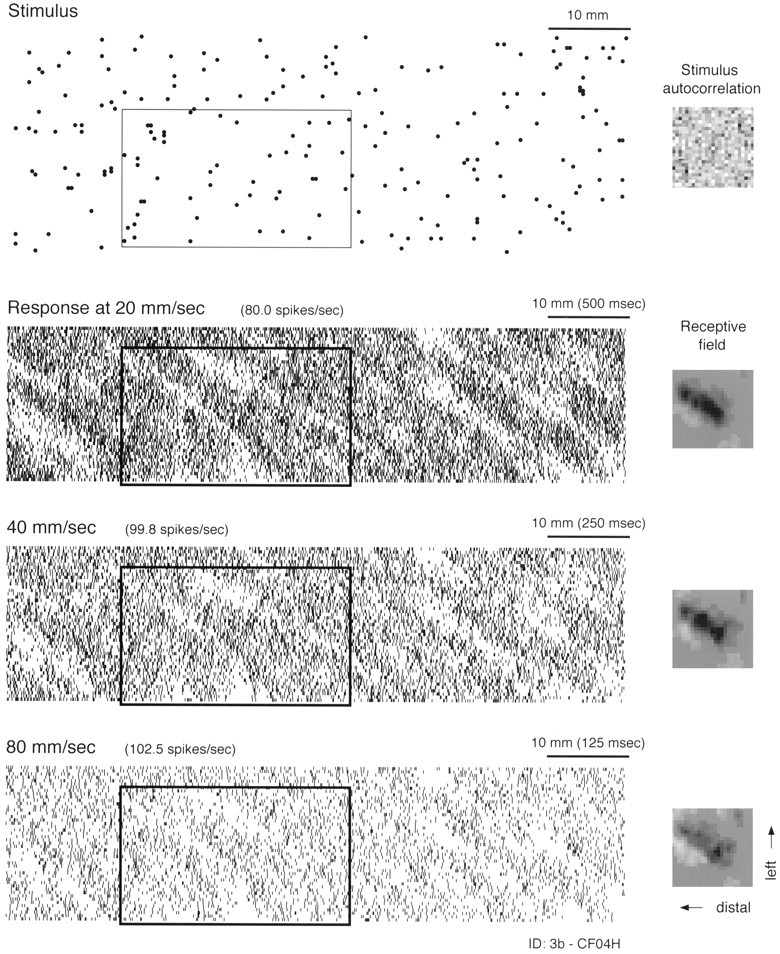
Responses. The interleaved data segments collected at 20, 40, and 80 mm/sec from each neuron were divided into three data sets, where each set was the response to the same pattern area (typically 10 × 175 mm) at a different scanning velocity. Within each of these three data sets, the action potentials were assigned two-dimensional (x,y) locations relative to the drum surface (Johnson and Phillips, 1988). The x location (distance in the scanning direction from the beginning of the random dot pattern) was determined by a digital shaft encoder. They location was determined by the axial (horizontal) position of the drum. Each of the three resulting spatial rasters is referred to as a spatial event plot (SEP). For example, Figure 3 shows SEPs of the three data sets collected from a single area 3b neuron.

Fig. 3.

Effect of scanning velocity on the response and RF of a single area 3b neuron. A portion of the random dot stimulus pattern is shown at the top. Each dotrepresents the location of a raised, truncated cone 400 μm in relief and 500 μm in diameter at the top. Cone locations were determined by a uniform, random number generator with a mean density of 10 dots/cm². The stimulus autocorrelation in thetop right shows that there was no significant patterning in the random dot locations (maximum correlation = 4.7% of center peak). The stimulus pattern scanned from right to left across the fingerpad. Responses at 20, 40, and 80 mm/sec are shown below the stimulus. Each tick marks the occurrence of a single action potential. The plotted position of each tick was determined by the location of the stimulus pattern at the instant the spike occurred (SEP). To the right is the RF determined from each SEP. Each RF is the map (25 × 25 bins = 10 × 10 mm of skin surface) of positive and negative weights that best describe (in a least squares sense) the neuron’s response at one scanning velocity (see Materials and Methods). Black regions are positive (excitatory); white regions are negative (inhibitory). Each RF is plotted as if viewing the surface of the glabrous skin through the back of the finger (i.e., from the neuron’s point of view) with the finger pointing to the left. Thus, the horizontal axis, proceeding from right toleft in each RF plot, represents position along the proximal-to-distal axis of the fingerpad (or increasing temporal delay), and the vertical axis represents space along the right–left axis of the finger as viewed through the back of the finger. The RFs reveal that this neuron is most sensitive to stimuli arranged in a slightly oblique, elongated region from NNE to SSW, and that the neuron is inhibited by dot stimuli on either side of this region. Examples of this stimulus selectivity are illustrated in theboxes overlaid on the stimulus and response plots.

Receptive field estimation. The pattern of firing evoked by the random dot stimulus at each scanning velocity was used to infer the two-dimensional pattern of RF excitation and inhibition on the skin surface (i.e., three RF estimates from each neuron). The details of the implementation are specified in our previous paper (DiCarlo et al., 1998). Here, we discuss the key theoretical features of the method and the reasons for adopting them. The broad outline is as follows: We use standard methods of multivariate regression (Draper and Smith, 1998) with a modification to account for the neuron’s threshold nonlinearity (inability to produce negative spike rates). The first step, which arises from the application of standard regression methods, is reverse correlation (stacking and averaging spike-triggered snapshots of the stimulus). However, stimulus autocorrelation distorts the RF obtained by this operation. Correction for this distortion is the purpose of the remaining steps of multivariate regression (solution of the normal equations). When the method stops after this step (reverse correlation) stimulus designs that minimize autocorrelation (e.g., white noise stimuli and M-sequences) are critical. When the method is carried to completion an unbiased estimate of the RF can be obtained from any stimulus as long as the dimensions of the space spanned by the stimuli exceed the number of RF parameters being estimated. The details as they apply in our study follow.

To describe the RF on the skin surface, we assumed that each small region of skin had a positive, negative, or zero effect on the firing rate when stimulated and that the instantaneous firing rate was equal to the sum of these effects. We subdivided a 10 × 10 mm square region of skin containing the RF into a grid of 625 (25 × 25) subregions, each 400 × 400 μm square. Multiple regression seeks the 625 positive (excitatory) and negative (inhibitory) values that, when convolved with the stimulus pattern, produce the best (least squared error) approximation to the observed firing rates.

The regression method has three parts. The first involves the standard, universal steps in formulating a multivariate model of a complex process. When there are insufficient data to construct a mechanistic model (which in this instance would be a model of the primary afferents, dorsal column nucleus, thalamic, and cortical circuitry underlying the responses we have observed), a widely used strategy for estimating complex input–output relationships is to use a stepwise, multivariate polynomial approximation (Marmarelis and Marmarelis, 1978). This approach starts with a linear model and successively adds higher-order interactions when they yield a significantly improved fit to the data (Draper and Smith, 1998). We showed in a previous paper that the first, linear step in this process accounts for 10–75% of the explainable response variance in area 3b neurons (DiCarlo et al., 1998). We have not included nonlinear terms in the RF model because they are generally not easily interpreted. The linear RF model that we have adopted,

$$\hspace{0.5em}{r}_{\text{linear}}(t)=b_0+b_1{x}_1(t)+b_2{x}_2(t)+b_3{x}_3(t)+\dots +b_{625}{x}_{625}(t),$$ Equation 1

approximates the response at all times, t, by a constant term, b₀, and the sum of the stimulus effects, x_i(t), at 625 subregions, which taken together span a skin region larger than any fingerpad RF that we have encountered in area 3b. The constantsb₁ to b₆₂₅ are zero when they represent locations where stimuli have no linear (additive or subtractive) effect on the response, positive at locations where stimuli produce (on average) an increase in firing rate, and negative at locations where stimuli produce a decrease in firing rate. The number of responses required for an adequate solution is larger than the number of unknown parameters (n = 626). Our stimulus procedure produces a response histogram with ∼20,000 responses (i.e., 20,000 bins). This yields 20,000 equations like the one above, which can be expressed as a matrix equation:

$$\mathbf{X}\mathbf{ }\mathbf{\text{b}}={\mathbf{\text{r}}}_{\text{linear}},$$ Equation 2

where X is the stimulus matrix (20,000 × 626),b is the vector of RF values (626 × 1), andr_linear is the predicted impulse rate at each time bin (20,000 × 1). Each row of X is a complete representation of the stimulus (within the 10 × 10 mm region specified above) at one time point.

The second step of the regression procedure, which we call zero removal, accounts for the fact that neurons cannot produce negative firing rates. If stimuli fall exclusively within the inhibitory part of the receptive field, the correct model will predict a large negative synaptic drive (i.e., a large negative r_linearvalue) but will be penalized for doing so if this negative drive is compared in a least squares manner with the observed impulse rate under those conditions (zero rate). To avoid this, we remove all the equations (rows of matrix Eq. 2) where an extended interval of zero firing indicates that the neuron is inhibited. A neural net with a thresholded activation function effectively does the same thing (Johnson et al., 1995). We used the multivariate regression procedure modified by zero removal because of its extensive theoretical foundations and the error analysis that it allows (Draper and Smith, 1998).

The third step of the regression procedure solves for the RF. It begins with reverse correlation and then corrects the result for the effects of stimulus autocorrelation. The RF parameters, b, that yield the best (in the least squared sense) approximation,r_linear, to the observed responses,r_observed, is obtained by solving the normal equation (Draper and Smith, 1998):

$$({\mathbf{X}}^T\mathbf{X})\mathbf{\text{b}}={\mathbf{X}}^T{\mathbf{\text{r}}}_{\text{observed}}.$$ Equation 3

The matrix operations effected on the right side of this equation, X^Tr_observed, are the operations of reverse correlation (de Boer and Kuyper, 1968; Jones and Palmer, 1987). The vector of 625 RF weights (plus a constant to account for the mean rate) that this operation produces is the sum of the stimulus snapshots (within the 10 × 10 mm region around the RF) when action potentials occurred. The matrix productX^TX is the stimulus autocorrelation matrix: each matrix element is the correlation between stimulus values at two locations in the RF. Consequently, the matrix product on the left side of the equation, (X^TX)b, is the convolution of the RF (i.e., b) with the stimulus autocorrelation function. Therefore, it can be seen that reverse correlation produces an estimate not of the RF but rather of the RF convolved with the stimulus autocorrelation function. Reverse correlation yields an uncontaminated (i.e., least squares) estimate of the RF only if the stimulus autocorrelation matrix is the identity matrix (i.e., the stimulus pattern within the RF estimation grid is uncorrelated with itself at all displacements). The standard regression method, which we have used, determines the best estimate of the RF in the general case by deconvolving the stimulus autocorrelation function and the result of reverse correlation:

$$\mathbf{\text{b}}=({\mathbf{X}}^T\mathbf{X}{)}^{-1} {\mathbf{X}}^T{\mathbf{\text{r}}}_{\text{observed}}.$$ Equation 4

In our case the stimulus pattern was obtained with a random number generator so that the pattern elements would be independent of one another at all displacements and that the off-diagonal terms of the autocorrelation matrix would be small. Therefore, the RFs that we display are not very different from those obtained with reverse correlation. However, that is no reason to forgo the deconvolution step. Every pattern obtained by random sampling is autocorrelated to some degree. Even stimulus sequences such as white-noise stimuli and M-sequences (Sutter, 1987) designed to minimize autocorrelation have some residual autocorrelation (Victor, 1992). The deconvolution step eliminates the concern that correlation in the stimulus may have affected the outcome. Furthermore, the deconvolution step allows a least squared error solution for any stimulus. Insofar as RF estimation is concerned, the only constraint on stimulus selection is the robustness of the stimulus autocorrelation matrix (Golub and Van Loan, 1989).

A final small but very important aspect of our method, which we used in our previous study (DiCarlo et al., 1998) as well as the current study, is the use of singular value decomposition (SVD) for the deconvolution (Golub and Van Loan, 1989). SVD provides a detailed description of the stimulus autocorrelation structure (i.e., its eigenvalues and eigenvectors). Because the deconvolution involves division by the eigenvalues of the stimulus autocorrelation function, the magnitude of those eigenvalues is critical. If any are near zero, they inordinately amplify errors in the RF resulting from noise or distortion in the response. In the SVD method those components can often be removed before solution to minimize distortion. In our case, the ratio of largest to smallest eigenvalues was 11.0, which is indicative of a robust RF solution (Golub and Van Loan, 1989), and no components of the deconvolution were removed.

Response alignment and measurement of temporal delays.Because there is an (initially) unknown delay between the stimulus and the neural response, alignment of the stimulus and the response is an issue; however, exact alignment between the stimulus pattern and the neural response is not critical. If the RF is estimated at two different alignments, the same RF weight pattern emerges, except that the pattern of excitatory and inhibitory weights is shifted within the 10 × 10 mm grid to reflect the difference in alignments. The important consideration is that the entire RF fit within the 10 × 10 mm grid. In this study, the alignment was adjusted so the center of excitation at 40 mm/sec was located at the center of the 10 × 10 grid. The same alignment was used to estimate the RFs at 20, 40, and 80 mm/sec. The conduction delay between skin stimulation and each RF component produces an apparent displacement of each RF component in the scanning direction that is proportional to the delay and the scanning velocity (see Appendix ). Because the scanning velocities are known, the delay can be estimated. The RF components estimated at 80 mm/sec will all be displaced in the scanning direction (to the left in the RF plots) relative to their position in the RF at 40 mm/sec; the RF components at 20 mm/sec will be displaced to the right relative to their position at 40 mm/sec. These relative displacements are used to estimate the excitatory and inhibitory delays (see Fig. 8); they can be seen on close inspection of the RFs in Figures 3-5.

Fig. 8.

Effect of scanning velocity on the locations of the dominant excitatory and inhibitory RF component centers. Thetwo left plots of the top row show the distal shifts of the apparent centers of excitation and inhibition relative to their locations at 20 mm/sec. The top right plot shows the differences between the inhibitory and excitatory shifts. The middle row shows the geometric means of the data in the top row (SEM brackets are too small to be seen). The bottom row contains histograms of the slopes of individual curves in the top row. In thetwo left columns, those slopes are estimates of the delay between skin stimulation and the centers of excitation and inhibition. The bottom right graph is the histogram of differences between the inhibitory and excitatory delays (see Results).

Fig. 4.

Effect of scanning velocity on the response and RF of a single area 3b neuron. See Figure 3. The RF of this neuron reveals that it is most sensitive to dots arranged in an oblique, elongated region from NW to SE. Examples of this stimulus selectivity are illustrated in the boxes overlaid on the stimulus and response plots.

Fig. 5.

Effect of scanning velocity on neural RFs. RFs computed from the responses of six area 3b neurons to stimuli scanned at 20, 40, and 80 mm/sec are shown on the left. The same RFs are shown in the center three columns withcircles to identify the regions of maximum excitation and inhibition, objectively determined (see Materials and Methods). The white circle in each RF identifies the region of maximum excitation; the black circleidentifies the region of maximum inhibition. The three columns at the right display cross-sections through the same receptive fields. The line defining each cross-section (illustrated in the corresponding center panel) passes through the centers of the circles defining the regions of maximum excitation and inhibition. Theordinate is the RF bin value, whose units represent impulses per second per millimeter of indentation at the indicated scanning velocity. The ordinates of the three histograms for each neuron are scaled to include the absolute peak value across all three scanning velocities (usually the excitatory RF peak at 80 mm/sec). The numbers above the upper and lower limits of the right-most graphs are the RF values represented by the extreme upper and lower ordinate values in each group of three histograms.

The delays associated with the dominant RF regions of excitation and inhibition were estimated by developing an objective method for identifying their centers. This was done by constructing two circles for each neuron, one for the excitatory region and one for the inhibitory region, and finding the locations in the RF that included the most excitation and inhibition. For excitation, the circle used to find the center of excitation had a radius proportional to the square root of the excitatory area (A_e):

$$r_{\text{e}}=\sqrt{A_{\text{e}}/2\pi }.$$ Equation 5

The excitatory portion of the RF rarely involved more than a single region and was generally circular or elliptical (DiCarlo et al., 1998). The circle described by this radius (r_e) typically encompassed one-third to one-half the total excitatory area depending on its eccentricity. Because the inhibitory regions were usually less concentrated, a slightly different algorithm was used to determine the appropriate radius. When inhibitory RF areas were less than ∼15 mm², they also consisted mainly of single compact regions, and the same procedure worked well. However, inhibitory regions with areas >15 mm² tended to be more elongated and often encompassed two or more sides of the excitatory region (e.g., Figs. 3, 5E). When the region is more elongated than circular, the radius required to encompass a constant fraction of the total area grows linearly with area. So, we devised a radius that grew as the square root of inhibitory area (A_i) up to 15 mm² and then gradually tended toward proportionality:

$$r_{\text{i}}=\left[\begin{array}{cc}r& \text{when} A_{\text{i}}<15 {\text{mm}}^2\\ r+(r-1.5{)}^2& \text{when} A_{\text{i}}\ge 15 {\text{mm}}^2\end{array}\right.$$

$$\text{where} r=\sqrt{A_{\text{i}}/2\pi }.$$ Equation 6

These inhibitory radii captured 20–50% of the inhibitory areas, depending on the shapes of the areas. The important point was to include sufficient volume to locate the centers of the most intense excitatory and inhibitory regions accurately while excluding the undue influence of distant points. The same excitatory and inhibitory radii (r_e and r_i determined at 20 mm/sec) were used for RF estimates at all three velocities for each neuron. The circle location enclosing the maximum excitatory (or inhibitory) mass was determined by complete search of all positions in each RF. Although the bin size of each RF was 400 × 400 μm, the precision was increased by shifting the circle in 50 μm increments (both directions) over the RF and including only the fraction of the mass in each bin that was within the circle.

Primary afferent recording. Recordings from primary afferents were performed on anesthetized rhesus monkeys (M. mulatta) weighing 4–5 kg using standard methods (Mountcastle et al., 1972). Single cutaneous mechanoreceptive fibers were dissected from the median or ulnar nerves. Afferents were classified as SA1, RA, or Pacinian on the basis of responses to indentation and vibration with a point probe (Talbot et al., 1968). Only SA1 and RA afferents with RFs located on one of the distal glabrous pads of digits 2–5 were studied. All stimulus, data collection, and RF analysis methods were the same as in the cortical experiments.

RESULTS

Eighty-four neurons in area 3b with RFs on a distal fingerpad were studied with random dot patterns scanned from proximal to distal across the fingerpad at 20, 40, and 80 mm/sec. These neurons were part of a larger sample (330 neurons) studied at 40 mm/sec (DiCarlo et al., 1998). A neuron with an RF located on one of the distal fingerpads was excluded from the study only if the finger and the stimulator could not be positioned to bring the RF, mapped with a manual probe, well within the contact region between the skin and stimulus surface. Even neurons that were marginally responsive to manual probing were studied with the idea that the random dot pattern might uncover responsiveness that was not evident with simpler probing.

Average firing rate versus scanning velocity

Figure 2 shows the mean impulse rates evoked by the random dot patterns at 20, 40, and 80 mm/sec. The distribution of rates among neurons was broad, with mean impulse rates varying by two orders of magnitude. In 90% of neurons, mean rates increased with increasing velocity (arithmetic mean rates, 20.0, 24.3, and 28.0 impulses/sec (imp/sec); geometric mean rates, 11.5, 14.4, and 16.3 imp/sec at 20, 40, and 80 mm/sec, respectively; SD = 0.47 log₁₀ units at all velocities). The slope of the log–log relationship between mean firing rate and scanning velocity for each of the 84 area 3b neurons is shown in the right panel of Figure 2. The mean slope is 0.252 (SD = 0.273), indicating that, on average, the mean firing rate of area 3b neurons increased by 19% as the scanning velocity doubled. With few exceptions, neurons with slopes <0 or >0.5 had response rates <10 imp/sec.

Fig. 2.

Effect of scanning velocity on firing rates. The graph on the left shows the mean firing rate of each area 3b neuron versus random dot scanning velocity. The graph on theright shows velocity sensitivity versus overall mean firing rate for individual neurons. The ordinate is the log–log slope of mean impulse rate versus velocity (1.0 indicates a linear, proportional relationship; 0.5, a square root relationship, etc.). The abscissa is the geometric mean impulse rate over all three velocities. Results from three primary afferent SA1 fibers (squares) and five primary afferent RA fibers (triangles) are shown for comparison.

The right panel of Figure 2 also shows the effect of scanning velocity on the mean firing rates of three SA1 and five RA primary afferents for comparison. Although the sample is small, the results are consistent with previous studies (Johnson and Lamb, 1981; Lamb, 1983; Phillips et al., 1992; Essick and Edin, 1995). The response rates of SA1 primary afferents, like those of area 3b neurons, increased only slightly as scanning velocity increased from 20 to 80 mm/sec (mean logarithmic slope = 0.302; SD = 0.020). RA primary afferents were more strongly affected by the same changes in scanning velocity (mean logarithmic slope = 0.668; SD = 0.106). As shown in Figure 2, the distribution of velocity effects on area 3b firing rates largely overlaps the velocity effects on SA1 but not RA firing rates.

Typical responses and RFs versus scanning velocity

Figure 3 shows response rasters of a typical area 3b neuron in the form of SEPs, where the horizontal axis represents space rather than time. The stimulus pattern segment illustrated in Figure 3 is ∼40% of the whole pattern (75 mm segment from the 175 mm pattern). Single sweeps across the pattern segment shown in Figure 3 represent time periods of ∼4, 2, and 1 sec at 20, 40, and 80 mm/sec, respectively. Although the impulse rate increased with increasing velocity, the increase was not enough to offset the greatly decreased scan times over each pattern segment. This accounts for the reduced spike density at higher velocities. Apart from this change in spike density, the spatial structure of the response was very similar across this fourfold change in scanning velocity, as can be seen by close comparison of the three SEPs. RF estimates based on the responses at the three scanning velocities are shown at the right sides of the SEPs.

The patterns of excitation and inhibition in the RFs at the three scanning velocities illustrated in Figure 3, like the response patterns, are largely unaffected by changes in scanning velocity. The three RF maps displayed in Figure 3 each reveal a large, central, slightly oblique region of excitation flanked by two regions of inhibition. In each RF map the excitatory and inhibitory regions are ovoid with a slight, oblique (NNE to SSW) orientation. This indicates that the neuron should respond best to dots in slightly oblique clusters regardless of scanning velocity. As predicted, wherever a cluster of this kind occurs (by chance), the neuron fires vigorously. The box in each SEP delineates the response to a region of the random dot pattern that happens to have several such clusters. Conversely, comparison of the stimulus pattern and the neural responses shows that this neuron responds poorly or not at all to clusters in the orthogonal (WNW to ESE) direction. Close inspection of this kind may give the impression that the stimulus pattern happens to be dominated by clusters of dots with a NNE to SSW orientation. However, this is not so, as indicated by two-dimensional autocorrelation of this 75 mm portion of the stimulus pattern, which is illustrated at the top right corner of Figure 3, and by the responses of other neurons that respond to clusters in other orientations within the same stimulus pattern (Fig. 4).

Figure 4 shows the responses of a neuron whose RF contains elongated regions of excitation and inhibition with orientations almost orthogonal to those of the previous example. Like the previous example, the neuronal responses and the RF estimates are very similar at the three scanning velocities. Unlike the previous example, the responses correspond to dot clusters with a dominant orientation in the NW to SE direction.

Figure 5 shows the RFs of six other area 3b neurons estimated at the three scanning velocities. These RFs and those shown in Figures 3 and 4 are typical examples of the effect of velocity on the RFs of area 3b neurons. Changes in velocity had several effects, which can be seen in these RF plots and are analyzed below: (1) the intensity of both excitation and inhibition increased with increasing scanning velocity; (2) the intensity of inhibition increased relative to excitation; and (3) the delay between the stimulus and the arrival of excitation and inhibition produced a progressive distal shift of the entire estimated RF location with increasing velocity. However, in each example, as in the larger sample of 84 neurons, a fourfold change in scanning velocity had no obvious effect on the spatial pattern of excitation and inhibition. This subjective assessment was supported by an analysis, which follows, of the pattern of RF excitation and inhibition of a subset of neurons whose RF estimates were sufficiently noise-free to allow precise, objective characterization of the spatial structures of their excitatory and inhibitory components.

RF structure

The structural similarity between RFs estimated at different scanning velocities was measured by computing the correlation between estimates. Pearson’s product–moment correlation coefficient computed on a bin-by-bin basis between any two RFs provides a powerful measure of their similarity; it compares all RF locations, and it is sensitive to changes in both the pattern and relative magnitudes of the excitatory and inhibitory effects, but it is unaffected by changes of scale that affect all values equally. A further reason for using correlation as a measure of structural similarity is that it was used in the previous study to measure differences between independent, repeated RF estimates at the same scanning velocity (DiCarlo et al., 1998). Because some of the lack of structural similarity between RFs at different velocities is due to RF noise, and we have measured this effect, we can separate the loss of correlation that is due to velocity effects from the loss due to noise in the repeated measures (see Appendix ).

We used an RF noise estimate developed in our previous study (DiCarlo et al., 1998) to restrict quantitative analyses to neurons whose RF estimates were relatively noise-free. Briefly, the raw estimate of each RF was filtered with a two-dimensional Gaussian filter whose SD (300 μm) was small relative to the spatial dimensions of interest. The noise removed by the Gaussian filter was measured as the SD of the difference between the raw and filtered RF estimates. The RF noise index was defined as the ratio of this SD to the peak filtered RF value. The previous study showed that very few RFs with noise indices <0.30 had correlations between repeated estimates <0.75 (i.e., they were highly repeatable). Because of the much longer time required to collect data at 20, 40, and 80 mm/sec than at 40 mm/sec alone (3.5 times longer), the collection time at 40 mm/sec was much shorter than in the previous study, and the RF estimates tended to be noisier. Thirty-four of the 84 neurons (40%) had RF noise indices <0.30 at 40 mm/sec, and the analyses of RF structure were restricted to these neurons. Because the collection time at 20 mm/sec was twice as long as at 40 mm/sec, and the number of action potentials was almost twice as great, the noise index was always lower at 20 mm/sec than at 40 mm/sec. This ensured highly reliable RF estimates from at least two scanning velocities.

Figure 6 illustrates correlation plots between RF estimates at 20, 40, and 80 mm/sec for a typical area 3b neuron (this neuron’s RFs are plotted in Fig. 3). Before plotting two RFs against one another on a bin-by-bin basis, the RF obtained at the slower velocity was shifted distally to compensate for the effects of conduction delay between skin stimulation and neural response (which averaged 15 msec; see later). This required a shift of one to three bins, depending on the difference in scanning velocities between the two RF estimates and the conduction delay. The correlation plots in Figure 6 show that the RF bins at all three scanning velocities were nearly colinear (correlations of 0.915, 0.884, and 0.873 for 20 vs 40 mm/sec, 40 vs 80 mm/sec, and 20 vs 80 mm/sec, respectively), indicating that the RFs determined at each of the scanning velocities have nearly identical patterns of excitation and inhibition. The correlation plots also show that both excitation and inhibition became more intense (larger RF bin values) as the scanning velocity increased. In the example shown in Figure 6, the excitatory and inhibitory weights at each RF location were approximately three times greater at 80 mm/sec than at 20 mm/sec.

Fig. 6.

Bin-by-bin comparisons of RF estimates obtained at three scanning velocities. The RF data are from the area 3b neuron illustrated in Figure 3. Each point in each plot represents bin values from corresponding bins in two RFs determined at two of the three velocities. Before comparison, the RFs were aligned to compensate for the small, progressive distal shifts produced by conduction delay between the stimulus and the response. In this case, the shifts were one, two, and four bins to the right at 20, 40, and 80 mm/sec (see Results). The bin values are in units of impulses per second per millimeter of indentation at the specified scanning velocity. The correlation coefficients from left toright were 0.915, 0.884, and 0.872.

Correlation coefficients between RFs obtained at 20 and 40 mm/sec and at 40 and 80 mm/sec are shown in Figure 7for each of the 34 neurons included in this analysis. The correlation values are all large, confirming that the spatial structure of each neuron’s RF is largely unaffected by changes in scanning velocity. Also, most points fall below the diagonal dashed line, indicating that RFs determined at 20 and 40 mm/sec are more similar than those at 40 and 80 mm/sec. However, that may simply reflect the fact that RF estimates are noisier at 80 than at 20 mm/sec, as discussed above. In fact, it is not clear that the data in Figure 7 signal any change in RF structure with changes in scanning velocity; the lack of perfect correlation could be attributable to RF noise alone.

Fig. 7.

Effect of scanning velocity on the RFs of area 3b neurons. Left, The ordinate is the correlation between RF estimates at 40 and 80 mm/sec. Theabscissa is the correlation between RF estimates at 20 and 40 mm/sec (see Fig. 6). Each point represents those two correlations for a single neuron. Right, Difference between observed correlations and expected correlations based on the null hypothesis that velocity had no effect on the pattern of excitation and inhibition in the RF. The method used to compute the expected correlation is explained in Appendix .

To test this hypothesis, we determined the correlation coefficient that would be expected between repeated RF estimates at two velocities if there was no change in the RF structure (see Appendix ). Figure 7shows the difference between the observed and expected correlation coefficients for each neuron (a negative difference indicates a loss of correlation greater than that expected from noise alone). The differences were distributed around zero, as can be seen in Figure 7, but in each pairing the mean was slightly negative (−0.028 for RFs at 20 and 40 mm/sec, −0.010 for 40 and 80 mm/sec, and −0.059 for 20 and 80 mm/sec). The difference was statistically significant (p < 0.01, t test) for 20 versus 40 and 20 versus 80 but not for 40 versus 80 mm/sec. These very slight but statistically significant differences are accounted for at least partially by a difference in the rate of growth of inhibition and excitation and a small growth of both excitatory and inhibitory area with increasing velocity (see below).

Excitatory and inhibitory delays

Because we have no a priori knowledge of the delay between a stimulus element and its excitatory or inhibitory effect on a neuron’s discharge, the RF analysis assigns the effect to the stimulus location at the time of the effect. Thus, the skin location that appears to produce the effect will be displaced from its true site of origin in the scanning direction by a distance that is proportional to the delay and the scanning velocity; that is, the slope of the relationship between this displacement and scanning velocity is the delay (see Appendix ). Because we can measure the locations of the centers of excitation and inhibition in the RF at each of the three velocities, we can measure this slope and, therefore, estimate the excitatory and inhibitory delays.

To do this, we sought an objective method for determining the locations of the main centers of excitation and inhibition within each RF estimate. Small regions of excitation or inhibition distant from the centers of excitation and inhibition, like outliers in statistics, can have an exaggerated effect on measures of location if they are included. Consequently, we adopted a measure of location, which, like statistically robust measures of central tendency, ignored the locations of distant data. The method consisted of constructing a circle that would capture, at most, 50% of the excitatory or inhibitory area at 40 mm/sec (see Materials and Methods) and searching the entire RF for the location that included the most excitatory or inhibitory mass within the circle. The center of that circle was taken as the center of excitation or inhibition. The important point was to include sufficient mass to locate the centers of the most intense excitatory and inhibitory regions accurately while excluding the undue influence of distant points. The excitatory mass included in this circle ranged from 33 to 50% of the total; the inhibitory mass ranged from 20 to 50%. The radii differed between neurons but were fixed within neurons at the value appropriate for the RF obtained at 20 mm/sec.

Results of the application of this algorithm are shown in Figure 5. The white cross is the location of the center of the (white) circle containing the most excitatory mass. The black cross (and circle) defines the location containing maximum inhibitory mass. This algorithm identified the same dominant excitatory and inhibitory foci at all three scanning velocities in 85% (29 of 34) of the neurons. Occasionally (5 of 34 neurons), when the RF contained two inhibitory regions of near-equal strength, the algorithm identified one region at two velocities and the other region at the other velocity; an example is shown in Figure 5F. These five neurons were eliminated from the analyses that follow.

Once the excitatory and inhibitory centers were located using the circular windows, we plotted the proximal-to-distal position of the centers and their relative proximal-to-distal separation as a function of velocity (Fig. 8). The distal location of each RF component is plotted as the offset from its proximal-to-distal location at 20 mm/sec. The top left and center panels of Figure 8 show that, with a few exceptions, the excitatory and inhibitory centers moved distally in the RF map as velocity increased from 20 to 80 mm/sec. The single neuron whose excitatory RF center was more proximal at 80 than at 20 mm/sec is the neuron shown in Figure 4. The explanation for this anomalous result can be seen by close inspection of the RFs in Figure 4. The excitatory field is large, and, although its overall boundaries shifted distally by a small amount, the increasing excitatory strength that occurred with increasing velocity (see later) occurred predominantly in the proximal part of the RF, causing the measured center of excitation to move proximally rather than distally. Similar effects explain the inhibitory responses that appear to have moved proximally with increasing velocity.

Because the distal offset caused by delay is the product of the delay and the scanning velocity (Eq. EA3), the slopes of the relationships between excitatory and inhibitory distal location and velocity illustrated in the top row of Figure 8 are direct estimates of the excitatory and inhibitory delays (see Appendix ). Those slopes for individual neurons are shown in the histograms in the bottom row of Figure 8. The mean excitatory and inhibitory delays, 15.5 and 11.4 msec, respectively, are both significantly different from zero (two-tailed t test, p < 0.001). These delays are consistent with previously reported response latencies in area 3b (Mountcastle and Powell, 1959; Gardner and Costanzo, 1980a).

The difference between excitatory and inhibitory distal offsets in individual neurons is displayed in the top right panel of Figure 8. Each point in this plot is the difference between points displayed in the middle and left top panels of Figure 8 for a single neuron. This plot shows that separation between excitatory and inhibitory centers in the scanning direction was not strongly affected by changes in scanning velocity. The distribution of the slopes of these lines is shown in the bottom right panel of Figure 8 and is expressed as the delay of the center of inhibition relative to the center of excitation. The mean of the distribution, −4.2 msec, is not significantly different from zero (p > 0.05, two-tailed t test). This result indicates that RF excitation and inhibition appear to act nearly simultaneously (i.e., without significant relative temporal delay) at scanning velocities between 20 and 80 mm/sec (but see Discussion).

RF mass

To investigate the effects of scanning velocity further and to compare the RFs described in this study with those in the previous study (DiCarlo et al., 1998), we analyzed RF area and mass. Excitatory (inhibitory) mass is a measure of the total strength of the excitatory (inhibitory) effects within the RF. As in the previous study, excitatory mass was calculated as the sum of the excitatory (positive) RF bin values, and inhibitory mass was calculated as the sum of the absolute values of the inhibitory (negative) RF bin values. Both excitatory and inhibitory mass have units of impulses per second per millimeter of stimulus relief, and both increased significantly with increasing scanning velocity (Fig. 9). The excitatory mass almost doubled between 20 and 80 mm/sec (geometric mean excitatory masses were 2937, 3810, and 5475 mass units at 20, 40, and 80 mm/sec, respectively). The inhibitory masses more than doubled (1897, 2925, and 4635 mass units at 20, 40, and 80 mm/sec, respectively). The mean slope of the logarithm of excitatory mass versus log velocity was 0.449 (SD = 0.306 log₁₀units); the comparable inhibitory slope was 0.644 (SD = 0.334 log₁₀ units). Both were significantly different from zero (p < 0.001, t test).

Fig. 9.

RF mass versus scanning velocity. Top panels show results for individual neurons; bottom panels show geometric means (brackets indicate SEM). Excitatory (inhibitory) mass was calculated as the sum of the values of the positive (negative) RF bins. The E/Iratio is the ratio of the total excitatory and inhibitory masses shown in the left two panels.

Relative changes in excitatory and inhibitory strength with changes in velocity were assessed by computing the ratios of excitatory to inhibitory mass, which are shown in the two right panels of Figure 9. At 40 mm/sec, the excitatory mass was, on average, 30% greater than the inhibitory mass (the geometric mean mass ratio was 1.302), which is consistent with the ratio in the larger sample (1.247) (DiCarlo et al., 1998). However, inhibition grew more rapidly than excitation with increasing scanning velocity, as indicated by a declining mass ratio (mean of slopes = −0.195; t = −2.75;p < 0.01). On average, the inhibitory mass grew from 65% of the excitatory mass at 20 mm/sec to 85% at 80 mm/sec. This effect is apparent on close inspection of the RFs shown in Figures3-5. In most of the RFs shown in these figures, some of the RF inhibition appears to deepen (i.e., become lighter on the RF plots) as scanning velocity increases. This effect of scanning velocity on the ratio of excitation to inhibition was particularly pronounced for the RF regions that trail the excitatory region (e.g., Figs. 3,5A).

RF area

As in the previous study (DiCarlo et al., 1998), the excitatory and inhibitory areas in each RF were calculated as the number of excitatory and inhibitory RF bins in the RF grid exceeding a threshold (10% of the peak excitatory or inhibitory value) and multiplied by the area covered by each RF bin (0.16 mm²). As in the larger study (DiCarlo et al., 1998), RF excitatory and inhibitory areas were both widely distributed (Fig. 10). The mean excitatory and inhibitory areas both grew 20% from 20 to 80 mm/sec (the geometric mean excitatory areas at 20, 40, and 80 mm/sec were 18.2, 18.7, and 21.8 mm², respectively; the inhibitory areas were 18.5, 20.4, and 22.2 mm², respectively). The mean excitatory and inhibitory areas at 40 mm/sec are slightly larger than the mean areas in the larger sample (14 and 18 mm², respectively; DiCarlo et al., 1998). The means of the slopes of log excitatory and inhibitory area versus log velocity were 0.131 (SD = 0.217) and 0.133 (SD = 0.303). Although slight, the mean slopes were statistically significant (excitatory:t = 3.50; p < 0.001; inhibitory:t = 2.55; p = 0.016). The ratio of excitatory RF area to inhibitory RF area, shown in the top right panel of Figure 10, is not affected by changes in scanning velocity (mean of slopes = 0.002; t = −0.31; p = 0.98).

Fig. 10.

RF area versus scanning velocity. Top panels show results for individual neurons; bottom panels show geometric means (brackets indicate SEM). Excitatory (inhibitory) area was calculated as the area covered by all the positive (negative) bins within the RF whose values exceeded 10% of the peak positive (negative) value. TheE/I ratio is the ratio of the total excitatory and inhibitory areas shown in the left two panels.

The growth of excitatory and inhibitory area provides a basis for estimating the persistence of excitation and inhibition in much the same way that progressive displacement of the centers of excitation and inhibition provided a basis for estimating the delay between the stimulus and excitation and inhibition. If, for example, the excitation persisted for 50 msec, the effect would be spread out over 1 mm at 20 mm/sec and over 4 mm at 80 mm/sec, which would have resulted in an increase of 3 mm in the proximal-to-distal RF dimensions. No growth of that magnitude was evident, so the persistence was obviously much less. This relationship between persistence and RF structure is analyzed in Appendix , where it is shown that the growth in excitatory and inhibitory area illustrated in Figure 10 is very close to that expected from excitatory and inhibitory persistence of ≤10 msec. If any part of the increase in measured area is attributable to an effect other than excitatory or inhibitory persistence (e.g., increased RF noise at the higher scanning velocities may result in some artifactual increase in RF area), then excitatory and inhibitory persistence is <10 msec.

Primary afferent RFs

Studies using complex spatial stimuli show that primary afferents, particularly SA1 afferents, exhibit response properties very much like those attributed to spatially separated excitation and inhibition in the CNS: skin indentation by any stimulus (e.g., a point, bar, or edge) evokes a smaller response when there is skin indentation at a neighboring region than when the stimulus indents the skin alone (Johnson and Lamb, 1981; Phillips and Johnson, 1981a; Phillips et al., 1992). This raises the question, what part of the area 3b RF inhibition reported here is attributable to the response properties of primary afferents? To address this, we studied 11 SA1 and 11 RA primary afferents using the same random dot patterns and RF estimation methods as were used in the cortical studies. Three SA1 and five RA afferents were studied using scanning velocities of 20, 40, and 80 mm/sec. The remainder were studied only at 40 mm/sec because of the abundant evidence that the spatial structure of primary afferent responses is unaffected by scanning velocity over the range from 20 to 80 mm/sec (Johnson and Lamb, 1981; Johnson et al., 1991; Phillips et al., 1992). Because the term inhibition implies synaptic mediation, we refer to the negative regions in primary afferent RFs as suppressive rather than inhibitory regions. The general features of SA1 and RA primary afferent RFs can be seen in the examples shown in Figure11. All 11 SA1 primary afferent fibers yielded RFs with regions of significant suppression that trailed behind the excitation, as can be seen in Figure 11 (i.e., the response evoked by a dot trailing closely behind another dot was suppressed relative to the response evoked by an isolated dot). The mean SA1 excitatory and suppressive areas at 40 mm/sec were 5.5 (range, 4.0–7.2) and 6.8 (range, 1.9–10.2) mm², respectively; the mean excitatory and suppressive masses were 4490 (range, 1530–7890) and 1920 (range, 640–2900) mass units, respectively. A suppressive region was detected in most RA afferents (9 of 11), but its magnitude was negligible compared with the excitation. The mean RA excitatory and suppressive areas at 40 mm/sec were 10.5 (range, 8.0–14.4) and 2.9 (range, 0–9.9) mm², respectively; the mean excitatory and suppressive masses were 6060 (range, 2570–9740) and 350 (range, 0–800) mass units, respectively. For comparison, the mean excitatory and inhibitory RF areas for the 247 area 3b neurons studied with the same random dot stimuli were 14.3 (range, 3–43) and 18.0 (range, 1–47) mm², respectively; the geometric mean excitatory and inhibitory cortical RF masses were 2140 (range, 210–10,300) and 1620 (range, 125–6830) mass units, respectively (DiCarlo et al., 1998). As in the area 3b RFs reported here, the spatial structure of the primary afferent RFs was largely unaffected by changes in scanning velocity. The excitatory mass increased with increasing scanning velocity for both afferent types, as did the suppressive mass for the SA1 afferents. These data indicate that some part of the trailing “inhibition” observed in area 3b RFs may be attributable to trailing suppression in the responses of SA1 but not RA afferents. However, none of the primary afferent RFs contained significant regions of suppression that did not trail the central excitation (e.g., as in Fig. 11). This indicates that nontrailing inhibitory regions in the area 3b RFs reported here and in the previous study (DiCarlo et al., 1998) must be attributable to mechanisms operating in the central pathways (i.e., dorsal column nucleus, thalamus, and/or SI cortex).

Fig. 11.

Effect of scanning velocity on typical SA1 and RA primary afferent RFs. The stimulus and methods used to determine the primary afferent RFs were identical to those used to determine the area 3b RFs in this study and the previous study (DiCarlo et al., 1998). The RF display is the same as in Figure 5.

DISCUSSION

The main result of this study is that the spatial structure of area 3b RFs is largely unaffected by changes in scanning velocity, but their excitatory and inhibitory intensities are affected strongly. Excitatory and inhibitory RF mass both nearly doubled as velocity increased from 20 to 80 mm/sec, and neural firing rates increased 42%. Correlations between RF estimates at different scanning velocities were often as high as correlations between repeated estimates at a single velocity. This indicates that the neural representation of a stimulus in area 3b is affected little by changes in scanning velocity. Analysis of the progressive shift in the apparent locations of the excitatory and inhibitory parts of the RFs with increasing velocity suggests that excitation and inhibition arrive nearly synchronously with a delay of ∼15 msec. Analysis of the growth of excitatory and inhibitory area showed that both components persist for 10 msec (SD) at most. Analysis of the RFs of primary afferents showed that some of the area 3b RF inhibition that trails behind the excitation might arise in the response properties of SA1 afferents.

Previous studies and mechanistic implications

Previous studies of the effect of scanning velocity on area 3b firing rates evoked by textured patterns (Burton and Sinclair, 1994;Tremblay et al., 1996) and brush stimuli (Whitsel et al., 1972; Essick and Whitsel, 1985) show that impulse rates generally rise with increasing scanning velocity. There are no previous studies of the effect of scanning velocity on the structure of somatosensory cortical RFs.

The results of this study considered in isolation would suggest that the excitatory and inhibitory effects that constitute the RF of an area 3b neuron arrive nearly synchronously, 10–15 msec after the stimulus that evokes them, and that their spatial structures are independent of scanning velocity. However, those inferences are consistent neither with the literature on the timing of excitation and inhibition in the somatosensory cortex nor with other results from our studies, which both suggest that some inhibition lags behind excitation. Previous studies indicate that there is substantial spatial overlap between excitatory and inhibitory effects (Laskin and Spencer, 1979; Gardner and Costanzo, 1980b) and that inhibitory effects are typically delayed relative to excitatory effects (Andersson, 1965; Whitehorn and Towe, 1968; Innocenti and Manzoni, 1972; Laskin and Spencer, 1979; Gardner and Costanzo, 1980b) by 10–20 msec (Laskin and Spencer, 1979; Gardner and Costanzo, 1980b). Our own studies (DiCarlo and Johnson, unpublished observations) show that when scanning direction is varied, area 3b RFs change shape in a way that suggests that some inhibitory effects are delayed relative to the excitatory effects. The question is how to reconcile these data and the results of the current study.

Figure 12 illustrates how overlapping excitation and inhibition can produce near-velocity invariance even when the inhibition is delayed substantially relative to excitation. The top two rows contain an exaggeratedly simplified RF model that illustrates the key points. The model consists of uniform, rectangular regions of excitation and inhibition that overlap in space but not in time: both the excitatory and inhibitory effects arise from the same skin region, but the inhibitory effect arrives 20 msec after the excitatory effect. When mapped with a scanned stimulus, this model matches qualitatively the RF features described in this study: (1) inhibition appears to trail excitation in the scanning direction (compare Figs. 3-5) because its temporal delay appears as a spatial offset in the scanning velocity (see Appendix ); (2) excitatory and inhibitory areas grow with increasing scanning velocity (compare Fig.10) because the increasing, apparent displacement between excitation and inhibition with increasing velocity reduces the cancellation between them; (3) net excitatory and inhibitory intensities (masses) increase with increasing scanning velocity (compare Fig. 9) for the same reason; and (4) the distance between the apparent centers of excitation and inhibition is fixed and independent of scanning velocity (compare Fig. 8) because it is determined by the widths of the overlapping excitation and inhibition, not by the temporal delay.

Fig. 12.

One- and two-dimensional models illustrating possible effects of scanning velocity on RF geometry. The purpose of these models is to show how inhibition can be delayed relative to excitation but result in either no shift of the center of inhibition relative to the center of excitation as scanning velocity varies (as inA) or only a minimal shift (as in B). The illustrative models assume inhibition whose origins on the skin overlap the region giving rise to excitation perfectly but whose effect is delayed by 20 msec relative to the excitation. Profiles above (below) the line in each panel represent profiles of excitation (inhibition). The horizontal axis in each panel represents the location on the skin surface where the excitation or inhibition appears to have arisen. When the stimulus moves at a constant velocity and there is an unknown delay between the stimulus event on the skin and the effect on the neuronal discharge, then the effect appears to have arisen from a location that is displaced from the true location by an amount proportional to the delay and the scanning velocity (see Appendix ). When the delay to inhibition is 20 msec greater than the delay to excitation, then the skin region giving rise to inhibition appears to be displaced by 0.02*velocity mm relative to the apparent location of the excitation (0.4 mm at 20 mm/sec, 1.6 mm at 80 mm/sec). A, The top row illustrates this effect at scanning velocities of 20 and 80 mm/sec in both the proximal and distal scanning directions. The second rowillustrates the net effect (i.e., the observed RF) after accounting for the canceling effects of overlapping excitation and inhibition (assumed to be additive). Rectangular profiles, 3 mm wide, are illustrated for simplicity. Note how the offset between the observed centers of excitation and inhibition is unaffected by changes in scanning velocity (compare Fig. 8) and how the observed excitatory and inhibitory volumes (masses) increase in intensity (compare Fig. 9). B, Same effects with Gaussian excitatory and inhibitory profiles meant to simulate more closely the RF profiles observed in this study. The inhibitory peak value is 10% less than the excitatory peak value, but its width is increased relative to the excitatory width so that they have equal mass. As in the simpler case illustrated above, the relative displacement between observed excitation and inhibition is affected little by changes in scanning velocity, and both excitation and inhibition become more intense with increasing velocity.C, Gray scale plots of the RFs that would be observed inB. The correlation of the RFs illustrated at 20 and 80 mm/sec is 0.95. The offset of the inhibition from the excitation is 2.3 mm at both 20 and 80 mm/sec, indicating apparent synchrony with the excitation (compare Fig. 8), whereas the actual relative delay was 20 msec.

The bottom two rows of Figure 12 are like the top two rows, except that the excitatory and inhibitory effects are more like the regions of excitation and in-field inhibition reported previously (Mountcastle and Powell, 1959; Gardner and Costanzo, 1980b). In this model, as in our results (compare Figs. 9, 10), net excitatory and inhibitory intensities (masses) increase much more with increasing velocity than do the excitatory and inhibitory areas. When the centers of excitation and inhibition and their displacements in the scanning direction are measured exactly the same way as in our study, the relative displacement between the centers is unchanged even though the relative displacement between the centers of the overlapped excitation and inhibition increased by 1.2 mm. If these data had been entered into our analysis of temporal delays (compare Fig. 8), we would have inferred that inhibition was synchronous with the excitation, whereas the true delay is 20 msec.

In summary, Figure 12 shows that overlapping excitation and inhibition can largely mask the effects of differences in delay between excitation and inhibition so that RF spatial structure is affected little by large changes in scanning velocity. However, this mechanism only accounts for the invariance of the relationship between excitation and trailing inhibition. Correlation analyses (Fig. 7) and visual inspection showed that the entire RF including “nontrailing” inhibitory regions was invariant, which suggests that a large part of the inhibition arrives synchronously with the excitation.

Primary afferent RF properties

Area 3b RF spatial and temporal structure is the result of peripheral as well as central mechanisms. Previous studies have shown that the spatial structure of SA1 and RA primary afferent responses to scanned dot patterns (Johnson and Lamb, 1981; Phillips et al., 1992), scanned embossed letters (Phillips et al., 1988; Johnson et al., 1991), and brushed stimuli (Edin et al., 1995) are unaffected over a wide range scanning velocities. Also, SA1 and RA impulse rates both rise with increasing raised pattern (Johnson and Lamb, 1981; Lamb, 1983;Phillips et al., 1992) and brushstroke (Whitsel et al., 1972; Franzen et al., 1984; Essick and Edin, 1995) velocity. Area 3b firing rates rise at nearly the same rate as primary SA1 firing rates and more slowly than primary RA firing rates (Fig. 2; Lamb, 1983; Phillips et al., 1992; Essick and Edin, 1995), which raises the intriguing possibility that area 3b neurons are driven largely by the SA1 primary afferent population and therefore are likely to play a critical role in form recognition (Johnson and Hsiao, 1992) and roughness perception (Blake et al., 1997a).

In the current study we showed that SA1 RFs have a trailing suppressive component that might contribute in part to the cortical inhibition that we have reported. In our previous study of area 3b RFs (DiCarlo et al., 1998), the inhibitory RF mass was, on average, almost as large (76%) as the excitatory mass. The mass of the SA1 trailing suppression averaged 43% of the excitatory mass, so a significant part, but not all, of the cortical trailing inhibition that we have reported could be accounted for by SA1 trailing suppression. Most RA RFs exhibited some trailing suppression, but its mass, 6% of the excitatory RA mass on average, was too small to account for more than a minor fraction of the cortical inhibition that we have reported.

SA1 and RA primary afferent transduction models based on homogeneous, isotropic elastic continua (Phillips and Johnson, 1981b; Srinivasan and Dandekar, 1996) provide a reasonable explanation of trailing suppression. The static skin deformation profile surrounding two dots separated by ∼3 mm in the scanning direction (the distance producing maximum trailing suppression) is like an inverted tent (with two supports) with deformation extending 3–4 mm in all directions from each of the dots (Phillips and Johnson, 1981b; Srinivasan, 1989; Connor et al., 1990; Phillips et al., 1992; Blake et al., 1997b). Both SA1 and RA afferents are much more sensitive to the rate of change of deformation than its absolute value (Pubols and Pubols, 1976). The rate of change of skin deformation is proportional to the spatial deformation gradient in the scanning direction and the velocity. Thus, an explanation for the reduced response to the trailing dot is that the skin is suspended between the dots, and therefore the spatial gradients leading up to the second dot are smaller than those leading up to the first dot (i.e., the indentation rates are less, and therefore the response is less).

The relative lack of trailing suppression in the RA RFs may have two explanations. One is that the RA RFs mapped by scanned dots are approximately twice as large as SA1 RFs (two times in the current study; Johnson and Lamb, 1981; Phillips et al., 1992) and that this masks any suppressive effect at a 3 mm separation. A second major factor is that RA but not SA1 afferents respond to the withdrawal of deformation (i.e., upward rate of deformation) (Talbot et al., 1968;Knibestöl, 1973; Pubols, 1980). Because the rate of withdrawal in the wake of the second dot is similar to the rate of indentation leading the first dot, the RA may respond well to both dots.

Functional implications of velocity invariance

The acquisition of tactile spatial information by scanning movements compensates for the very limited field of view provided by a single fingerpad. It is clearly an advantage to be able to scan one’s fingers over an object or a surface rapidly without loss of spatial acuity. However, temporal factors such as reduced time in which to respond to each stimulus element at higher scanning velocities, differences in latency between different response components, persistence of excitatory and inhibitory effects, and even conduction velocity dispersion in the afferent pathways (Johnson and Lamb, 1981) tend to degrade the spatial integrity of a moving neural image. Nonetheless, psychophysical experiments demonstrate little loss of spatial acuity at scanning rates from 20 mm/sec up to at least 80 mm/sec (Vega-Bermudez et al., 1991). This, in turn, implies that mechanisms at all levels within the pathways leading to perception maintain the integrity of spatial information over this broad range of scanning velocities. The increased firing rates that accompany increased scanning velocities compensate to some extent for the reduced dwell time over each stimulus feature. The primary significance of overlapping inhibition and excitation in the neural RFs may be to minimize the effects of differences in delay between the excitatory and inhibitory components of the RF. Whether this is so or not, the data presented here demonstrate that area 3b responses are essentially invariant over a wide range of scanning velocities. This invariance is consistent with the hypothesis that area 3b plays a critical role in tactile spatial perception, including roughness estimation and form recognition, which are also unaffected by changes in scanning velocity (Katz, 1925; Lederman, 1974, 1983; Vega-Bermudez et al., 1991).

Relationship between a neuron’s full spatiotemporal RF and its RF estimated with a scanned stimulus

In this appendix we derive the relationship between the neuron’s true spatiotemporal RF and the RF that we have estimated with a scanned stimulus in this and the previous study (DiCarlo et al., 1998). We assume that except for the threshold nonlinearity that arises because a neuron cannot produce a negative discharge rate, the mechanisms are linear. If they are not, the formulation applies to the response fraction that is accounted for by linear mechanisms. The instantaneous discharge rate, r(t), produced by a general stimulus that varies in both time and space,s(x,y,t), is determined by the weighting assigned to all the stimuli that affect its discharge (e.g., Marmarelis and Marmarelis, 1978):

$$r(t)=\underset{-\infty }{\overset{\infty }{\int }} \underset{-\infty }{\overset{\infty }{\int }} \underset{0}{\overset{\infty }{\int }} s(x,y,t-\tau )w(x,y,\tau )d\tau \text{dxdy},$$ Equation A1

when the result is positive and zero otherwise. The weighting function w(x,y,τ) is the neuron’s spatiotemporal RF, which describes the effect of stimulation of each location (x,y) in the neuron’s RF at each time lag (τ) after the stimulus was presented. When a stimulus pattern with constant spatial structure,p(u,v), is scanned across the RF at a constant velocity, the stimulus within the RF at any instant of time is given by s(x,y,t) =p(x₀ + x −v_xt, y₀ +y − v_yt), wherex₀ and y₀ specify the stimulus location in contact with the center of the RF at timet = 0. The object is to determine the unknownw(x,y,τ). However, the two-dimensional data provided by neural responses to a pattern scanned at a single velocity and scanning direction are not sufficient to determine the three-dimensional structure ofw(x,y,τ) (because spatial and temporal effects are confounded in the scanning direction). To see this, we define new variables: x′ = x +v_x τ and y′ = y +v_y τ. Then, by substituting x′ −v_x τ for x and y′ −v_y τ for y, the convolution integral (Eq. EA1) can be reformulated as:

$$r(t)=\underset{-\infty }{\overset{\infty }{\int }} \underset{-\infty }{\overset{\infty }{\int }} p(x_0+x^{\prime }-v_{x}t,y_0+y^{\prime }-v_{y}t)h(x^{\prime },y^{\prime }){\text{dx}}^{\prime }{\text{dy}}^{\prime }$$ Equation A2

$$\text{where} h(x^{\prime },y^{\prime })=\underset{0}{\overset{\infty }{\int }}w(x^{\prime }-v_x\tau ,y^{\prime }-v_y\tau ,\tau )d\tau ;$$

h(x′,y′) is the two-dimensional RF that we have estimated at v_x = 20, 40, and 80 mm/sec and v_y = 0.

The effects of delay and persistence can be seen by examining the RF estimates produced by scanning a stimulus across a spatiotemporal, excitatory RF that is Gaussian in space and time [i.e., by assuming that w(x,y,τ) in Eq. EA1 is a three-dimensional Gaussian]. Assume the spatial distribution of the Gaussian is described by a center (μ_x,μ_y) and the spread by (ς_x and ς_y), and that it has a mean delay of τ_delay (temporal “center”), and persistence characterized by a temporal spread, ς_t. We assume a scanning velocity, v, in the x direction. They′ dimensions of the two-dimensional RF obtained by integrating the three-dimensional RF are the same as forw(ς_y′ = ς_y). The mean location and spread in the x direction are given by:

$${\mu }_{x^{\prime }}={\mu }_x+{\nu }_x{\tau }_{\text{delay}}$$

$${\varsigma }_{x^{\prime }}=\sqrt{{\varsigma }_x^2+{\nu }_x^2{\varsigma }_t^2}.$$ Equation A3

The shift of the RF component caused by temporal delay is manifested in the product,v_x*τ_delay, in Equation EA3. Larger delays or larger scanning velocities produce larger shifts in the RF component from its true spatial center (μ_x). If the delay is assumed to be constant, then Equation EA3 shows that the slope of the measured spatial center (μ_x′) versus velocity is a direct measure of the delay (see Fig. 8). The smearing of the RF component caused by persistence is manifested in the product,v_x²*ς_t², in Equation EA3. Larger temporal persistence or larger scanning velocities produces larger spatial extent in the measured RF spread (ς_x′). Our method of calculating RF area (all RF regions exceeding 10% of the peak value) includes all RF area within ±2.15 SD of the center of a Gaussian RF; thus the area of the measured RF h(x′,y′) is:

$$\text{area}=(2.15{)}^2·\pi ·{\varsigma }_x^{\prime }·{\varsigma }_y^{\prime }.$$ Equation A4

A typical excitatory area of 20 mm² (see Fig.10) would be produced by ς_x = ς_y = 1.2 mm. The growth in area produced by persistence can be seen by examining the effect of various persistence values, ς_t. In fact, a persistence of 10 msec (ς_t = 10 msec) matches the observed increases in RF area closely. It predicts a 4% growth in area between 20 and 40 mm/sec and 20% growth between 20 and 80 mm/sec. The observed increases in area were 3 and 20% for excitatory area and 10 and 20% for inhibitory area.

Compensation for velocity effects unrelated to RF structure

Changes in scanning velocity had two effects on the estimated RF unrelated to its structure, and we took measures to compensate for both effects in the computation of RF correlation. One was progressive RF displacement in the scanning direction with increasing velocity because of conduction delays between the stimulus and the cortex. This effect is accounted for as described in Results. The other was an increase in RF noise with increasing scanning velocity because of the reduced recording times at higher velocities. When the scanning velocity doubled (e.g., from 20 to 40 imp/sec) the mean impulse rates increased, on average, by 25%, but the recording time was cut in half. As a result, the number of action potentials entering into the RF estimate at the higher velocity dropped by 38% on average, and the noise in the RF estimates increased substantially. The null hypothesis is that scanning velocity had no effect on the spatial structure of the RFs and therefore that the decline in correlation between two estimates at different scanning velocity is determined by the noise in the two estimates. The following is the method used to determine the expected correlation when the noise levels in the two estimates are different.

The previous paper showed that repeated RF estimates based on data from interleaved sweeps at the same scanning velocity were highly correlated and that the correlation coefficient was related in a systematic way to the RF noise index, which is illustrated in Figure13. It is difficult to imagine any systematic differences in the RF related to the interleaved sweeps, so we assume that the loss of correlation (values <1.0) was entirely due to noise in the two RF estimates that entered into each correlation value. If the noise indices of the two RF estimates obtained at different velocities were similar, the expected correlation could be obtained from Figure 13, but they typically were not, as indicated above. However, the expected correlation can still be estimated as the product of the square roots of the correlations associated with each of the noise indices. That relationship is derived as follows.

Fig. 13.

Correlations of repeated estimates of the same RF (from DiCarlo et al., 1998). The ordinate represents the correlation of two independent estimates of the same area 3b RF obtained from alternating sweeps of the random dot pattern across the RF at 40 mm/sec. The abscissa represents the average noise index of the two RF estimates (see DiCarlo et al., 1998, Results). The solid line is a running average produced by a 100-point-wide boxcar filter.

Each RF estimate can be written as the sum of RF signal (i.e., the expected value of the RF bins) and RF noise (i.e., fluctuations in the RF bins caused by variability in the neural processes leading up to the spikes from which the RF is estimated):

$$RF(i)=S(i)+N(i)i=1,2,\dots 625.$$ Equation B1

where RF(i) is the estimate in the ith RF bin, S(i) is the expected (i.e., true) RF value in the ith bin, and N(i) is the noise in the estimate of the ith RF bin. Defined this way, the noise (N) is uncorrelated with the signal (S) so that the variance of the observed RF is equal to the sum of their individual variances:

$${\varsigma }_{RF}^2={\varsigma }_S^2+{\varsigma }_N^2.$$ Equation B2

The expected Pearson’s correlation coefficient of any two RF estimates, RF₁ and RF₂, is:

$${\rho }_{12}=\frac{\text{cov}({RF}_1,{RF}_2)}{\text{var}({RF}_1{)}^{1/2} \text{var}({RF}_2{)}^{1/2}}$$ Equation B3

$$=\frac{\text{cov}(S_1+N_1,S_2+N_2)}{({\varsigma }_{S_1}^2+{\varsigma }_{N_1}^2{)}^{1/2}({\varsigma }_{S_2}^2+{\varsigma }_{N_2}^2{)}^{1/2}}$$

$$=\frac{\text{cov}(S+N_1,S+N_2)}{({\varsigma }_S^2+{\varsigma }_{N_1}^2{)}^{1/2}({\varsigma }_S^2+{\varsigma }_{N_2}^2{)}^{1/2}}$$

$$=\frac{{\varsigma }_S^2}{({\varsigma }_S^2+{\varsigma }_{N_1}^2{)}^{1/2}({\varsigma }_S^2+{\varsigma }_{N_2}^2{)}^{1/2}}.$$

We have assumed by the null hypothesis that two RFs estimated from the same neuron at different scanning velocities have identical underlying structure (i.e., S₁ =S₂ = S). When the noise variances are identical, as we assume they are in estimates based on interleaved sweeps at the same velocity, the correlation between estimates of the same RF (RF₁ vs RF₁) is given by:

$${\rho }_{11}=\frac{{\varsigma }_S^2}{({\varsigma }_S^2+{\varsigma }_{N_1}^2)}.$$ Equation B4

Thus, it can be seen that the expected correlation between two estimates of the same RF with different noise variances (Eq. EB3 above) is given by:

$${\rho }_{12}={\left(\frac{{\varsigma }_S^2}{{\varsigma }_S^2+{\varsigma }_{N_1}^2}\right)}^{1/2}{\left(\frac{{\varsigma }_S^2}{{\varsigma }_S^2+{\varsigma }_{N_2}^2}\right)}^{1/2}$$ Equation B5

$$={\rho }_{11}^{1/2} {\rho }_{22}^{1/2},$$

where ρ₁₁ and ρ₂₂ are the expected correlations for repeated measures of RFs with noise variances ς₂^N₁ and ς₂^N₂. The noise variances are not known but the noise indices are, and they can be used to get estimates of the expected correlations for repeated RF estimates (ρ₁₁ and ρ₂₂).

To do this, the data in Figure 13 were smoothed using a 100-point-wide boxcar filter; the result is shown as a solid line. For each RF estimate at each scan velocity, an estimate of the correlation coefficient of that RF and another RF estimate obtained under identical stimulus conditions (i.e., ρ₁₁ in Eq. EB5) was determined using the noise index of the RF estimate and the curve in Figure 13. Thus, for two RFs estimated from the same neuron at different scanning velocities, the expected correlation under the null hypothesis of identical underlying RF structures but possibly different noise variances (i.e., ρ₁₂ in Eqs. EB3 and EB5) was determined from Equation EB5, with ρ₁₁ and ρ₂₂determined from the noise indices of each RF estimate.

REFERENCES

- 1.Andersson SA. Intracellular postsynaptic potentials in the somatosensory cortex of the cat. Nature. 1965;205:297–298. doi: 10.1038/205297a0. [DOI] [PubMed] [Google Scholar]
- 2.Blake DT, Hsiao SS, Johnson KO. Neural coding mechanisms in tactile pattern recognition: the relative contributions of slowly and rapidly adapting mechanoreceptors to perceived roughness. J Neurosci. 1997a;17:7480–7489. doi: 10.1523/JNEUROSCI.17-19-07480.1997. [DOI] [PMC free article] [PubMed] [Google Scholar]
- 3.Blake DT, Hsiao SS, Johnson KO. Monkey cutaneous SA1 and RA responses to raised and depressed scanned patterns: effects of width, height, orientation, and a raised surround. J Neurophysiol. 1997b;78:2503–2517. doi: 10.1152/jn.1997.78.5.2503. [DOI] [PubMed] [Google Scholar]
- 4.Burton H, Sinclair RJ. Representation of tactile roughness in thalamus and somatosensory cortex. Can J Physiol Pharmacol. 1994;72:546–557. doi: 10.1139/y94-079. [DOI] [PubMed] [Google Scholar]
- 5.Connor CE, Hsiao SS, Phillips JR, Johnson KO. Tactile roughness: neural codes that account for psychophysical magnitude estimates. J Neurosci. 1990;10:3823–3836. doi: 10.1523/JNEUROSCI.10-12-03823.1990. [DOI] [PMC free article] [PubMed] [Google Scholar]
- 6.de Boer E, Kuyper P. Triggered correlation. IEEE Trans Biomed Eng. 1968;15:169–179. doi: 10.1109/tbme.1968.4502561. [DOI] [PubMed] [Google Scholar]
- 7.DiCarlo JJ, Lane JW, Hsiao SS, Johnson KO. Marking microelectrode penetrations with fluorescent dyes. J Neurosci Methods. 1996;64:75–81. doi: 10.1016/0165-0270(95)00113-1. [DOI] [PubMed] [Google Scholar]
- 8.DiCarlo JJ, Hsiao SS, Johnson KO. Structure of receptive fields in area 3b of primary somatosensory cortex in the alert monkey. J Neurosci. 1998;18:2626–2645. doi: 10.1523/JNEUROSCI.18-07-02626.1998. [DOI] [PMC free article] [PubMed] [Google Scholar]
- 9.Draper NR, Smith H. Applied regression analysis, Ed 3. Wiley; New York: 1998. [Google Scholar]
- 10.Edin BB, Essick GK, Trulsson M, Olsson KA. Receptor encoding of moving tactile stimuli in humans. I. Temporal pattern of discharge of individual low-threshold mechanoreceptors. J Neurosci. 1995;15:830–847. doi: 10.1523/JNEUROSCI.15-01-00830.1995. [DOI] [PMC free article] [PubMed] [Google Scholar]
- 11.Essick GK, Edin BB. Receptor encoding of moving tactile stimuli in humans. II. The mean response of individual low-threshold mechanoreceptors to motion across the receptive field. J Neurosci. 1995;15:848–864. doi: 10.1523/JNEUROSCI.15-01-00848.1995. [DOI] [PMC free article] [PubMed] [Google Scholar]
- 12.Essick GK, Whitsel BL. Factors influencing cutaneous directional sensitivity: a correlative psychophysical and neurophysiological investigation. Brain Res Brain Res Rev. 1985;357:213–230. doi: 10.1016/0165-0173(85)90025-6. [DOI] [PubMed] [Google Scholar]
- 13.Franzen O, Thompson FJ, Whitsel BL, Young M. Peripheral coding mechanisms of touch velocity. In: von Euler C, Franzen O, Lindblom U, Ottoson D, editors. Wenner-Gren International Symposium series, Vol. 41, Somatosensory mechanisms. Macmillan; London: 1984. pp. 213–226. [Google Scholar]
- 14.Gardner EP, Costanzo RM. Spatial integration of multiple-point stimuli in primary somatosensory cortical receptive fields of alert monkeys. J Neurophysiol. 1980a;43:420–443. doi: 10.1152/jn.1980.43.2.420. [DOI] [PubMed] [Google Scholar]
- 15.Gardner EP, Costanzo RM. Temporal integration of multiple-point stimuli in primary somatosensory cortical receptive fields of alert monkeys. J Neurophysiol. 1980b;43:444–468. doi: 10.1152/jn.1980.43.2.444. [DOI] [PubMed] [Google Scholar]
- 16.Gardner EP, Costanzo RM. Neuronal mechanisms underlying direction sensitivity of somatosensory cortical neurons in awake monkeys. J Neurophysiol. 1980c;43:1342–1354. doi: 10.1152/jn.1980.43.5.1342. [DOI] [PubMed] [Google Scholar]
- 17.Golub GH, Van Loan CF. Matrix computations, Ed 2. Johns Hopkins UP; Baltimore: 1989. [Google Scholar]
- 18.Innocenti GM, Manzoni T. Response patterns of somatosensory cortical neurones to peripheral stimuli. An intracellular study. Arch Ital Biol. 1972;110:322–347. [PubMed] [Google Scholar]
- 19.Johnson KO, Hsiao SS. Tactual form and texture perception. Annu Rev Neurosci. 1992;15:227–250. doi: 10.1146/annurev.ne.15.030192.001303. [DOI] [PubMed] [Google Scholar]
- 20.Johnson KO, Lamb GD. Neural mechanisms of spatial tactile discrimination: neural patterns evoked by Braille-like dot patterns in the monkey. J Physiol (Lond) 1981;310:117–144. doi: 10.1113/jphysiol.1981.sp013540. [DOI] [PMC free article] [PubMed] [Google Scholar]
- 21.Johnson KO, Phillips JR. A rotating drum stimulator for scanning embossed patterns and textures across the skin. J Neurosci Methods. 1988;22:221–231. doi: 10.1016/0165-0270(88)90043-x. [DOI] [PubMed] [Google Scholar]
- 22.Johnson KO, Phillips JR, Hsiao SS, Bankman IN. Tactile pattern recognition. In: Franzen O, Westman J, editors. Information processing in the somatosensory system. Macmillan; London: 1991. pp. 305–318. [Google Scholar]
- 23.Johnson KO, Hsiao SS, Twombly IA. Neural mechanisms of tactile form recognition. In: Gazzaniga MS, editor. The cognitive neurosciences. MIT; Cambridge, MA: 1995. pp. 235–268. [Google Scholar]
- 24.Jones JP, Palmer LA. The two-dimensional spatial structure of simple receptive fields in cat striate cortex. J Neurophysiol. 1987;58:1187–1211. doi: 10.1152/jn.1987.58.6.1187. [DOI] [PubMed] [Google Scholar]
- 25. Katz D. The world of touch. Reprint (Krueger LE, translator). 1925. Erlbaum; Hillsdale, NJ, 1989 [Google Scholar]
- 26.Knibestöl M. Stimulus-response functions of rapidly adapting mechanoreceptors in the human glabrous skin area. J Physiol (Lond) 1973;232:427–452. doi: 10.1113/jphysiol.1973.sp010279. [DOI] [PMC free article] [PubMed] [Google Scholar]
- 27.Lamb GD. Tactile discrimination of textured surfaces: peripheral neural coding in the monkey. J Physiol (Lond) 1983;338:567–587. doi: 10.1113/jphysiol.1983.sp014690. [DOI] [PMC free article] [PubMed] [Google Scholar]
- 28.Laskin SE, Spencer WA. Cutaneous masking. II. Geometry of excitatory and inhibitory receptive fields of single units in somatosensory cortex of the cat. J Neurophysiol. 1979;42:1061–1082. doi: 10.1152/jn.1979.42.4.1061. [DOI] [PubMed] [Google Scholar]
- 29.Lederman SJ. Tactile roughness of grooved surfaces: the touching process and the effects of macro- and microsurface structure. Percept Psychophys. 1974;16:385–395. [Google Scholar]
- 30.Lederman SJ. Tactual roughness perception: spatial and temporal determinants. Can J Psychol. 1983;37:498–511. [Google Scholar]
- 31.Marmarelis PZ, Marmarelis VZ. Analysis of physiological systems: the white noise approach. Plenum; New York: 1978. [Google Scholar]
- 32.Mountcastle VB, Powell TP. Neural mechanisms subserving cutaneous sensibility, with special reference to the role of afferent inhibition in sensory perception and discrimination. Bull Johns Hopkins Hosp. 1959;105:201–232. [PubMed] [Google Scholar]
- 33.Mountcastle VB, LaMotte RH, Carli G. Detection thresholds for stimuli in humans and monkeys: comparison with threshold events in mechanoreceptive afferent nerve fibers innervating the monkey hand. J Neurophysiol. 1972;35:122–136. doi: 10.1152/jn.1972.35.1.122. [DOI] [PubMed] [Google Scholar]
- 34.Mountcastle VB, Reitboeck HJ, Poggio GF, Steinmetz MA. Adaptation of the Reitboeck method of multiple microelectrode recording to the neocortex of the waking monkey. J Neurosci Methods. 1991;36:77–84. doi: 10.1016/0165-0270(91)90140-u. [DOI] [PubMed] [Google Scholar]
- 35.Phillips JR, Johnson KO. Tactile spatial resolution: II. Neural representation of bars, edges, and gratings in monkey primary afferents. J Neurophysiol. 1981a;46:1192–1203. doi: 10.1152/jn.1981.46.6.1192. [DOI] [PubMed] [Google Scholar]
- 36.Phillips JR, Johnson KO. Tactile spatial resolution: III. A continuum mechanics model of skin predicting mechanoreceptor responses to bars, edges, and gratings. J Neurophysiol. 1981b;46:1204–1225. doi: 10.1152/jn.1981.46.6.1204. [DOI] [PubMed] [Google Scholar]
- 37.Phillips JR, Johnson KO, Hsiao SS. Spatial pattern representation and transformation in monkey somatosensory cortex. Proc Natl Acad Sci USA. 1988;85:1317–1321. doi: 10.1073/pnas.85.4.1317. [DOI] [PMC free article] [PubMed] [Google Scholar]
- 38.Phillips JR, Johansson RS, Johnson KO. Responses of human mechanoreceptive afferents to embossed dot arrays scanned across fingerpad skin. J Neurosci. 1992;12:827–839. doi: 10.1523/JNEUROSCI.12-03-00827.1992. [DOI] [PMC free article] [PubMed] [Google Scholar]
- 39.Pubols BH., Jr On- versus off-responses of raccoon glabrous skin rapidly adapting cutaneous mechanoreceptors. J Neurophysiol. 1980;43:1558–1570. doi: 10.1152/jn.1980.43.6.1558. [DOI] [PubMed] [Google Scholar]
- 40.Pubols BH, Jr, Pubols LM. Coding of mechanical stimulus velocity and indentation depth by squirrel monkey and raccoon glabrous skin mechanoreceptors. J Neurophysiol. 1976;39:773–787. doi: 10.1152/jn.1976.39.4.773. [DOI] [PubMed] [Google Scholar]
- 41.Srinivasan MA. Surface deflection of primate fingertip under line load. J Biomech. 1989;22:343–349. doi: 10.1016/0021-9290(89)90048-1. [DOI] [PubMed] [Google Scholar]
- 42.Srinivasan MA, Dandekar K. An investigation of the mechanics of tactile sense using two-dimensional models of the primate fingertip. J Biomech Eng. 1996;118:48–55. doi: 10.1115/1.2795945. [DOI] [PubMed] [Google Scholar]
- 43.Sutter E. A practical nonstochastic approach to nonlinear time-domain analysis. In: Marmarelis VZ, editor. Advanced methods of physiological system modeling. University of Southern California; Los Angeles: 1987. [Google Scholar]
- 44.Talbot WH, Darian-Smith I, Kornhuber HH, Mountcastle VB. The sense of flutter-vibration: comparison of the human capacity with response patterns of mechanoreceptive afferents from the monkey hand. J Neurophysiol. 1968;31:301–355. doi: 10.1152/jn.1968.31.2.301. [DOI] [PubMed] [Google Scholar]
- 45.Tremblay F, Ageranioti-Bélanger SA, Chapman CE. Cortical mechanisms underlying tactile discrimination in the monkey. I. role of primary somatosensory cortex in passive texture discrimination. J Neurophysiol. 1996;79:3382–3403. doi: 10.1152/jn.1996.76.5.3382. [DOI] [PubMed] [Google Scholar]
- 46.Vega-Bermudez F, Johnson KO, Hsiao SS. Human tactile pattern recognition: Active versus passive touch, velocity effects, and patterns of confusion. J Neurophysiol. 1991;65:531–546. doi: 10.1152/jn.1991.65.3.531. [DOI] [PubMed] [Google Scholar]
- 47.Victor JD. Nonlinear systems analysis in vision: overview of kernel methods. In: Pinter RB, Nabet B, editors. Nonlinear vision. CRC; Ann Arbor, MI: 1992. pp. 1–37. [Google Scholar]
- 48.Whitehorn D, Towe AL. Postsynaptic potential patterns evoked upon cells in sensorimotor cortex of cat by stimulation at the periphery. Exp Neurol. 1968;22:222–242. doi: 10.1016/0014-4886(68)90053-8. [DOI] [PubMed] [Google Scholar]
- 49.Whitsel BL, Roppolo JR, Werner G. Cortical information processing of stimulus motion on primate skin. J Neurophysiol. 1972;35:691–717. doi: 10.1152/jn.1972.35.5.691. [DOI] [PubMed] [Google Scholar]