Asymmetric Suppression Outside the Classical Receptive Field of the Visual Cortex

Abstract

Areas beyond the classical receptive field (CRF) can modulate responses of the majority of cells in the primary visual cortex of the cat (Walker et al., 1999). Although general characteristics of this phenomenon have been reported previously, little is known about the detailed spatial organization of the surrounds. Previous work suggests that the surrounds may be uniform regions that encircle the CRF or may be limited to the “ends” of the CRF. We have examined the spatial organization of surrounds of single-cell receptive fields in the primary visual cortex of anesthetized, paralyzed cats. The CRF was stimulated with an optimal drifting grating, whereas the surround was probed with a second small grating patch placed at discrete locations around the CRF. For most cells that exhibit suppression, the surrounds are spatially asymmetric, such that the suppression originates from a localized region. We find a variety of suppressive zone locations, but there is a slight bias for suppression to occur at the end zones of the CRF. The spatial pattern of suppression is independent of the parameters of the suppressive stimulus used, although the effect is clearest with iso-oriented surround stimuli. A subset of cells exhibit axially symmetric or uniform surround fields. These results demonstrate that the surrounds are more specific than previously realized, and this specialization has implications for the processing of visual information in the primary visual cortex. One possibility is that these localized surrounds may provide a substrate for figure–ground segmentation of visual scenes.

Areas beyond the classical receptive field (CRF) have been studied extensively for cells in the primary visual cortex (Hubel and Wiesel, 1965; Maffei and Fiorentini, 1976;Knierim and Van Essen, 1992; Li and Li, 1994; Lamme, 1995; Sillito et al., 1995). Although a variety of effects have been described, and several hypotheses have been advanced, the functional utility of the surround is still not clear. A potentially major impediment to our understanding of this phenomenon is the limited attention given to the spatial organization of the surround.

Previous research on surround interactions is segregated into three groups, based on the portion of the surround that is stimulated. Most attention has been given to the end zones (Hubel and Wiesel, 1965;Rose, 1977; Kato et al., 1978; Orban et al., 1979a,b; Bolz and Gilbert, 1986; Knierim and Van Essen, 1992; DeAngelis et al., 1994; Li and Li, 1994), whereas others have studied the side zones (Glezer et al., 1973;Albus and Fries, 1980; De Valois et al., 1985; Born and Tootell, 1991;Knierim and Van Essen, 1992; DeAngelis et al., 1994; Li and Li, 1994) or used stimuli that encircle the CRF (Blakemore and Tobin, 1972;Maffei and Fiorentini, 1976; Nelson and Frost, 1978; Knierim and Van Essen, 1992; Li and Li, 1994; Lamme, 1995; Sillito et al., 1995; Zipser et al., 1996; Sengpiel et al., 1997). The conclusions from these studies are limited because of the unsubstantiated assumptions regarding the nature of RF surround organization. We have undertaken the study reported here to provide detailed information concerning the spatial organization of the RF surround. Our assumption is that understanding the spatial organization of the surround is an important step toward uncovering its functional role.

In this paper, we investigate the detailed spatial organization of the RF surround. Using careful controls in the experiments, we find that all surround interactions are suppressive in nature. We do not find evidence of facilitation in the surrounds. Second, the surrounds are typically asymmetrical, with only a small portion providing the inhibitory signal. Third, we find that the location of the suppressive portion of the surround can arise at any location and is not limited to the ends or sides, although there is a slight bias toward end zone suppression.

MATERIALS AND METHODS

Physiological preparation. We describe here the methods used to explore the spatial organization of CRF surrounds of individual cortical cells. Briefly, experiments were conducted using anesthetized, paralyzed cats. Thirty minutes before anesthesia, acepromazine maleate (0.5 mg/kg) and atropine sulfate (0.06 mg/kg) are injected subcutaneously to provide tranquilization and to suppress secretion, respectively. Anesthesia is induced and maintained during surgery with 2–4% isoflurane. Forepaw femoral veins are cannulated for intravenous infusion; a tracheal tube and a rectal thermometer are inserted; and electrocardiographic (ECG) leads and electroencephalographic (EEG) screw electrodes are positioned. A craniotomy (∼5 mm in diameter) is performed around Horsley–Clarke coordinates P4L2, and the dura is carefully removed. Two tungsten-in-glass (Levick, 1972) microelectrodes are positioned just above the surface of the cortex at an angle of ∼10° medial and 20° anterior, and the hole is covered with agar and sealed with wax to form a closed chamber.

During recording, animals are artificially respirated at ∼25 strokes/min with a mixture of N₂O (70%) and O₂ (30%). Anesthesia and paralysis are maintained by intravenous infusion of a mixture of thiopental sodium (Pentothal, 2.5% solution; 1.4 mg · kg⁻¹ · h⁻¹) and gallamine triethiodide (Flaxedil, 2% solution; 9.4 mg · kg⁻¹ · h⁻¹), combined with a 5% dextrose and lactated Ringer's solution (0.5 ml · kg⁻¹ · h⁻¹). Steady-state hydration is provided by a drip system through which lactated Ringer's is infused (10 ml · kg⁻¹ · hr⁻¹). Temperature is maintained near 38°C, and end-tidal CO₂ at 4–4.5%. EEG, ECG, heart rate, core body temperature, and expired CO₂ are monitored continuously through a personal computer (PC)-based physiological monitoring and analysis system (Ghose et al., 1995). The pupils are dilated with 1% atropine sulfate, and nictitating membranes are retracted with 5% phenylephrine hydrochloride. Contact lenses (+2D) with 3 mm artificial pupils are placed on both corneas. Every 8–12 hr, the contact lenses are removed and cleaned, and the clarity of the refractive media is checked with a direct ophthalmoscope. Chloromycetin (1.50 ml/d) is given intravenously every 12 hr as a prophylactic. The location of the optic disk in each eye is plotted on a tangent screen with a reversible direct ophthalmoscope. From the positions of the optic disks, we can infer the spatial location of the area centrales as 14.6° temporal and 6.5° inferior (Bishop et al., 1962).

Experimental apparatus. Visual stimuli are displayed on a tangent screen in front of the animal or on two separate cathode ray tube (CRT) displays (Nanao T2–17), allowing independent stimulation of each eye via a half-silvered beam splitter. A manually controlled joystick is used in preliminary tests of the RF to sweep a bar stimulus of variable size and orientation in any position and direction on the tangent screen.

A visual stimulator generates images on each CRT display independently. The stimulator consists of a PC with two high-resolution graphics boards (Imagraph) and runs software written in our laboratory. The frame refresh rate of each CRT display is 76 Hz, and both displays are refreshed synchronously. Stimuli are delivered with a temporal resolution of one frame period (13.2 msec) by custom temporal modulation driver software. The spatial resolution is 1024 × 804 pixels. The usable portion of the display subtends an area of 28 × 22° (viewed at 57 cm), and the mean luminance at the front surface of each contact lens is 23 cd/m².

The microelectrodes are inserted through the pia via a guide tube and advanced through the cortex by a piezoelectric micropositioner (Burleigh). Custom-made digital signal-processing software is used to discriminate individual action potentials. This software allows accurate and reliable discrimination of individual spikes from multiple cells on each electrode. After discrimination, each action potential is recorded as a binary event, time-stamped with 1-msec accuracy, and stored for off-line analysis.

Recording procedures. When a cell is encountered and the spike waveform is isolated, the location and approximate orientation preference of the CRF are determined. Next, we use an interactive search program (DeAngelis et al., 1993) to determine suitable parameters for a circular patch of drifting sinusoidal grating presented on one of the CRT displays. In this procedure, the grating patch is presented on the CRT, and the size, orientation, and spatial frequency of the grating are adjusted by the experimenter until preferred values are determined. This procedure is used for each eye, and the values obtained are used as initial stimulus parameters for subsequent runs.

Quantitative CRF tests. For quantitative analysis of the CRF, grating stimuli are presented monocularly for 4 sec at a time (temporal frequency, 2 Hz for all gratings) in blocks of randomly interleaved trials. The size of the stimulus for these initial presentations is typically 5–8° in diameter. Each stimulus is presented at least four times, and successive presentations are separated by 3 sec during which the animal views blank screens of the same mean luminance as the gratings. After presentation of a complete set of stimuli, the DC (mean rate) and first harmonic (at 2 Hz) components of the accumulated response are computed for each stimulus using discrete Fourier analysis. We define response amplitude as the greater of the mean firing rate or the amplitude of the first harmonic of the response. Simple and complex cell designations are determined by classical criteria (Hubel and Wiesel, 1962) and by the ratio of the first harmonic and mean of the response to a drifting grating stimulus (Skottun et al., 1991).

To determine the orientation tuning of the CRF, we present a series of drifting grating stimuli, differing in orientation around the initial orientation estimate. For this run, the spatial frequency and size are set to the initial values obtained using the search program. The peak of the resultant tuning curve is used as the optimal orientation for subsequent presentations. In a similar manner, we determine the preferred spatial frequency for the cell.

The optimal orientation, spatial frequency, and size for CRF stimulation were determined quantitatively for each cell from the preliminary runs described above. Throughout this paper the phraseoptimal stimulus is used to refer to a drifting grating with orientation, spatial frequency, and size parameters set to the values that elicit the greatest response from the cell. The contrast was set at an intermediate value that varied from cell to cell but was typically ∼35%. Sinusoidal gratings were drifted for four seconds at a temporal frequency of 2 Hz. After the optimal stimulus was determined for each cell, the size of the CRF was estimated by presenting a drifting grating within a circularly bounded window of variable size. The resultant size-tuning curve yields an estimate of the spatial dimensions of the CRF and also the degree of surround suppression (Walker et al., 1999).

Detailed spatiotemporal maps of the CRF were also obtained for some cells using either the reverse correlation (DeAngelis et al., 1993) or m-sequence (Sutter, 1992; Anzai et al., 1997) methods. These maps were used to verify the accuracy and reliability of the parameters obtained with grating stimuli. One particular advantage of these maps is that they provide very accurate information about the center and size of the CRF, which is critical to success in a study of surround properties. In general, there is excellent agreement between the grating and noise measurements.

Surround stimulation. The primary goal of this study is to determine the spatial organization of inhibitory regions beyond the CRF. Measuring inhibition directly in neurons of area 17 is difficult because of the low spontaneous levels of activity in most cells. To overcome this problem, an optimal center stimulus is used to provide a baseline excitatory drive for the cell, and small grating stimuli are placed at a number of locations around the CRF (Fig.1). The positions of the surround patches are aligned on axes that correspond to the preferred orientation of the cell. The ends of the CRF are defined as the regions beyond the CRF that lie along the axis of preferred orientation, and thesides correspond to the regions lying outside of the CRF on an axis perpendicular to the preferred orientation. We useoblique to refer to the regions that are in between the ends and sides of the CRF. Figure 1B indicates the relative positions and sizes of the surround patches used. The sizes of the surround patches were chosen so that they overlapped partially with each other and thus completely tile the surround space. Eight positions were used typically, although in some early experiments, only four surround positions were used, and these patches were proportionately larger and placed at each end and side of the CRF. A small gap was always placed between the center and surround gratings. This gap provides an extra measure of insurance against the possibility that the surround gratings encroach on the CRF. The spatial phase of the central and surround gratings was matched, although it has been previously shown that relative phase differences do not affect the strength of surround suppression (DeAngelis et al., 1994).

Fig. 1.

Illustration of our method for investigating the CRF surrounds. All four of these configurations (A–D) are interleaved in a single stimulation set. The CRF is indicated by the rectangle, and theline extending through it denotes the preferred orientation. A, A central grating patch is set to the optimal orientation, spatial frequency, position, and size for each CRF. This stimulus provides a baseline response rate from the cell.B, The surround is investigated by placing the optimal stimulus in the center and presenting small circular patches of drifting gratings in areas beyond the CRF at a variety of locations equidistant from the center of the CRF. The dashed circles indicate the patch locations used in a typical experiment, although only one surround location was stimulated at a time. Unless otherwise noted, the parameters of the surround patch matched those of the center patch and differed only in size and location. A small gap of uniform mean luminance (typically 0.5°) was placed between the surround grating and the central grating.C, As a control measure, the center was stimulated along with an annulus in the surround in which the spatial extent of the annulus covers a region that is the sum of all of the small surround gratings. D, The surround annulus was presented alone to ensure that it does not produce excitation in the cell. Although not illustrated, we also presented the small surround patches by themselves at all locations. The peristimulus time histogram to theleft of each diagram is the response obtained from seven repetitions from one cell in this study (cell 436-13; more of this cell shown in Fig. 4).

A series of control conditions were interleaved with the main trials to provide periodic baseline measurements for the response to the optimal stimulus as well as to ascertain the overall effect of surround stimulation and ensure that the surround stimuli were not driving the cell. One control was the optimal stimulus, presented alone within the CRF region, which established the baseline response level for the cell (Fig. 1A). A second control was the presentation of an annular surround in conjunction with the optimal center stimulus, where the spatial extent of the annulus was the same as the sum of the smaller surround patches (Fig. 1C). This control provided a measure of the overall effect of the surround. Finally, the annular surround (Fig. 1D) and the smaller surround patches were presented alone, to ensure that they did not produce an excitatory response from the cells. This control is crucial, because a criticism that can be levied against many surround studies is that one cannot be certain that the “surround” stimuli are truly in the surround. A lack of response during this control is taken as strong evidence that the stimuli are outside of the CRF.

In sum, a complete set of stimulus configurations includes the smaller surround patches presented at each location shown in Figure1B with and without the center stimulation and two presentations each of the control conditions shown in Figure 1,A, C, and D. This entire block of presentations is repeated eight times on average (range, 4–28), which provides an average of 16 measures for each control. In addition, a “null” condition is included, in which activity is recorded during viewing of a blank screen to estimate the spontaneous activity.

RESULTS

Cell population

Measurements were made from 271 cells in 19 adult cats. Of these, 133 were classified as simple and 138 as complex, according to classical criteria (Hubel and Wiesel, 1962) and also to the ratio of the first harmonic to DC response rate (Skottun et al., 1991). These 271 cells represent an unbiased, random sampling of cells from all layers (Walker et al., 1999). The presence of surround suppression was examined in all of these neurons, and the spatial organization was fully explored in a subset of 101 cells (65 simple and 36 complex). Most of these cells were chosen because they exhibited relatively strong surround suppression, although several cells without obvious surround suppression were also tested. Unless otherwise noted, the results presented in this paper were compiled using only the dominant eye data, although a few cells were studied through both eyes.

The size-tuning curves described in a related paper (Walker et al., 1999) are excellent predictors of the likelihood of observing surround suppression with the small surround grating patches. As expected, neurons exhibiting suppression for large patch sizes showed commensurate suppression when examined with small, discrete surround gratings as well. Consequently, we usually concentrated on cells that exhibited marked suppression in the size-tuning curves. However, there are also reports of facilitation from the surrounds (Maffei and Fiorentini, 1976; Nelson and Frost, 1978; Kapadia et al., 1995; Sillito et al., 1995; Rossi et al., 1996; Levitt and Lund, 1997; Sengpiel et al., 1997; Polat et al., 1998). In addition, recent psychophysical and theoretical studies suggest that stimuli outside of the CRF can augment the response to stimuli in the center (Field et al., 1993; Polat and Sagi, 1993, 1994; Kapadia et al., 1995; Stemmler et al., 1995; Polat and Norcia, 1996). Because of these factors, we periodically conducted further tests with neurons that lacked obvious suppression to large stimuli in the size-tuning data. We considered the possibility that facilitation and suppression might originate from separate discrete locations and cancel each other when large stimuli cover the entire surround. With small surround stimuli, we attempted to reveal any antagonistic pockets of inhibition and excitation from the surround for cells with no apparent suppression in their size-tuning curves. However, strong surround modulation was never observed from a cell that lacked suppression in the size-tuning estimation, nor did we observe facilitation. On the basis of these observations, we refined the protocol to include only those cells that exhibited size-tuning suppression of at least 40%. Forty percent is an arbitrary value chosen because it provides clear evidence of suppression, which in turn allows for definitive analysis of the surround structure. Whereas the 271 cells described in a related study (Walker et al., 1999) represent an unbiased sample of striate neurons (mean surround suppression is 27.88% ± 31.10 SD), the sample used in this study of surround spatial organization is more representative of cells exhibiting moderate to strong surround suppression (mean percent suppression with large annular stimuli, 38.82% ± 31.47 SD).

Unless otherwise noted, all data were obtained with the orientation and spatial frequency of the surround gratings matched to the optimal for the CRF. We refer to this as the optimal surround stimulus. Thus, the optimal surround does not necessarily imply a high response rate or maximum degree of suppression from the surround; rather, it designates that the orientation of the surround grating was set to the optimal for the CRF.

Asymmetric surround suppression

Typically, we observed that only a limited portion of the surround exerts an influence on the response of a cell. Consider, for example, the spatial profiles of the surrounds of three typical neurons shown in Figure 2. Each rowpresents data from a single cell. Results are displayed in polar plots, where the spatial location of the small surround patches is given by the polar angle, and the radial value indicates the response rate. All plots are rotated so that the preferred orientation lies along thevertical axis (the accompanying rectangle depicts the true orientation and preferred direction of motion for each CRF). Thus, the ends (E) and sides (S) of the CRF are located along the vertical and horizontal axes, respectively. Figure 2 illustrates cells in which stimulation of a single end or side of the CRF produces exactly the same amount of suppression as that obtained by stimulating the entire surround.

Fig. 2.

Examples of surround asymmetry for three cells. All of these responses were obtained with the central and surround gratings set to the preferred orientation for the CRF. The radial axis is the response rate (spikes per second). The angular position indicates the position of the small surround patch (see Fig.1B). The outer dashed circle is the baseline response to center stimulation alone, measured on separate, interleaved trials. The gray region around this circle represents ±SEM. The mean response to stimulation of the center and annular surround ± SEM is indicated by a solid circle and lighter gray shading (e.g., seeC, D) but is not visible if the response is suppressed to near spontaneous levels (e.g., see A, B). If there is ongoing spontaneous activity, it is indicated by acircle and a dark shaded region (±SEM). All plots have been rotated so that the preferred orientation of the cell is vertical, with the preferred direction of motion to theright. The ends (E) and sides (S) are denoted on each plot. The tilted rectangle next to the plot indicates the true orientation and direction preference of the cell. The filled data pointsconnected by the solid line represent the mean response to stimulation of the CRF plus one of the small surround patches. Error bars denote ±1 SEM. The unfilled data points are control responses measured during presentation of the small surround gratings alone. These conditions ensure that our surround patches are truly beyond the CRF and do not drive the cell and, therefore, elicit responses near the spontaneous level of the cell. Thearrow extending outward from the origin is the SI vector (see Results), normalized to the scale of the radial axis for each cell. Thus, an SI₁ vector with a value of 1.0 indicates complete asymmetry and would extend to the edge of the polar plot. For all three cells, the left plot shows the responses when the surround is mapped with four surround locations, and theright plot is obtained during a separate presentation with eight surround locations. A, B, Surround maps from a complex cell. Note that the overall pattern of suppression is equivalent in both of these measures and that the SI₁values are similar. C, D, Surround maps from a simple cell with suppression from one side of the CRF. Again, the overall spatial pattern of surround suppression is similar in the two measures, although it is apparent that the suppressive region can also be activated by surround patches placed in the oblique regions to the left of the CRF. E, F, Complex cell with suppression from one end of the CRF. Surr., Surround.

Figure 2 also demonstrates the compatibility of data collected with four and eight surround locations. The left column presents data collected with four locations, and the right columncontains data from the same cells but collected from eight locations. Figure 2A shows the response from a complex cell that was strongly suppressed by the annular surround and also by a small grating patch placed at one end of the CRF. Approximately 2 hr later, the surround was probed again, this time with smaller surround patches placed at eight separate spatial locations. The result of this mapping is shown in Figure 2B. The same spatial pattern is evident, and an intermediate degree of suppression is seen from the adjacent patches on either side of the location at which maximum suppression is observed. This suggests that the two adjacent patches stimulated only a portion of the surround inhibitory zone, whereas the position just beyond the “bottom” end of the CRF activated the most of the suppressive zone. Because the surround gratings slightly overlap spatially (see Fig. 1B), the suppressive zone appears to be limited to a region that covers approximately the same spatial area as a single surround patch (3.5° in this example).

The plots in Figure 2, C and D, show a pair of measurements made from a simple cell. The measurements were made ∼1 hr apart, and again, there is excellent agreement between the two plots, even though the overall responsiveness of the cell diminished slightly over time. In the first measurement (Fig. 2C), the overall suppression is 50.2% with the annular surround stimulus. Note that the same degree of suppression is observed when a single small grating patch is placed on one side of the CRF. In this example, an intermediate amount of suppression is also generated by the patch located just “below” the end of the CRF, although the other end and side of the CRF has no effect on the response to the optimal center stimulus. Figure 2D shows that even though the response has decreased and the variability has increased (e.g.,wider shaded circle), the overall percent suppression (60.8%) and spatial organization remain very similar to the original plot shown in Figure 2C.

The surround asymmetry from another complex cell is shown in Figure 2,E and F. The cell shows strong suppression from one end and modest facilitation from one side (Fig.2E). The data displayed in Figure2F were collected ∼45 min later and show the same pattern of suppression from one end. In Figure 2F, mild suppression is observed at two positions adjacent to the primary suppressive region in addition to strong suppression from the small grating patch placed at one end of the CRF. Notice that even though the suppression pattern is equivalent in the two repeated measurements, the facilitation from the left side is not preserved, suggesting that this facilitation is probably artifactual.

The examples shown in Figure 2 are representative of the cells in the population with respect to the asymmetry of surround suppression and the repeatability of the measurements made with four or eight surround locations. Although the plots with eight surround locations yield higher spatial resolution, the maps with four surround positions require less time to run and provide adequate measures of the location and strength of the surround suppressive zones. For some cells, the only measurements obtained were from trials with four surround locations, and these cells are included in the data set because they give accurate information about the suppressive surround region. For data obtained from both four and eight surround locations, the eight-position data are always used for subsequent analysis and summary statistics.

Quantification of asymmetry

It is apparent from the examples in Figure 2 that the surround inhibitory fields can be spatially asymmetric. In addition to suppression arising from the ends or sides, it will be shown that suppression can be concentrated in any region of the surround. A metric was developed to quantify the spatial organization of the surround and to describe the degree of asymmetry in individual surround locations. The metric originates from circular statistics methodology (Batschelet, 1981) and has been applied in similar analyses of CRF asymmetry in extrastriate middle temporal area (MT) (Xiao et al., 1995). A suppression index (SI₁) was computed for each cell using the following formula:

$$\Vert {SI}_1\Vert =\frac{\sqrt{{\left(\sum _{\text{i}}^n{S}_{\text{i}}\times sin({\alpha }_{\text{i}})\right)}^2+{\left(\sum _{\text{i}}^n{S}_{\text{i}}\times cos({\alpha }_{\text{i}}\right)}^2}}{\sum _{\text{i}}^n{S}_{\text{i}}},$$ Equation 1

where S_i is the magnitude of suppression at each surround location, α_i. It is helpful to think of each surround location as being described by a vector pointing in that direction with a length that is proportional to the strength of suppression. Then, SI₁ is the magnitude of the vector that results from summing the suppression vectors from all surround locations, normalized to the total length of all the suppression vectors. SI₁ attains a value of 1.0 if all of the suppression arises from a single surround location and is 0.0 if the suppression is equally balanced among all surround locations.

Occasionally, there was evidence of axially symmetric suppression (i.e., suppression arising from two opposing regions of the CRF). This pattern of suppression yields SI₁ values close to zero. Thus, a second index, SI₂, was computed to describe suppression exhibiting an axial symmetry. Equation 1 was used to compute SI₂, but each position angle (α_i) was doubled. Thus, SI₂ is largest (1.0) when all suppression originates along a single axis, such as suppression occurring exclusively on the two ends. An SI₂ value of 0.0 indicates that the cumulative suppression along each axis is equal.

To quantify the surround location with the most suppression, the angle of the suppression index vector is computed with the following equation:

$$\text{ang}(SI)=\text{arctan}\left(\frac{\sum _{\text{i}}^n{S}_{\text{i}}\times sin({\alpha }_{\text{i}})}{\sum _{\text{i}}^n{S}_{\text{i}}\times cos({\alpha }_{\text{i}})}\right).$$ Equation 2

Note that for SI₂, this angle indicates theaxis of strongest suppression.

SI₁ values are indicated on all polar plots as the vector extending radially outward from the origin (except Figs. 7and 10A–C, which show SI₂). The vector points to the area of the surround with the strongest suppression, as computed from Equation 2. The length of the vector is determined by Equation 1, and, for plotting purposes, is normalized to the maximum response rate used in each plot. Thus, if a cell has complete asymmetry, with suppression originating exclusively from one region, the vector will extend to the outer edge of the plot. If there is no suppression, or if it is symmetrically balanced, the vector will remain close to the origin.

Fig. 7.

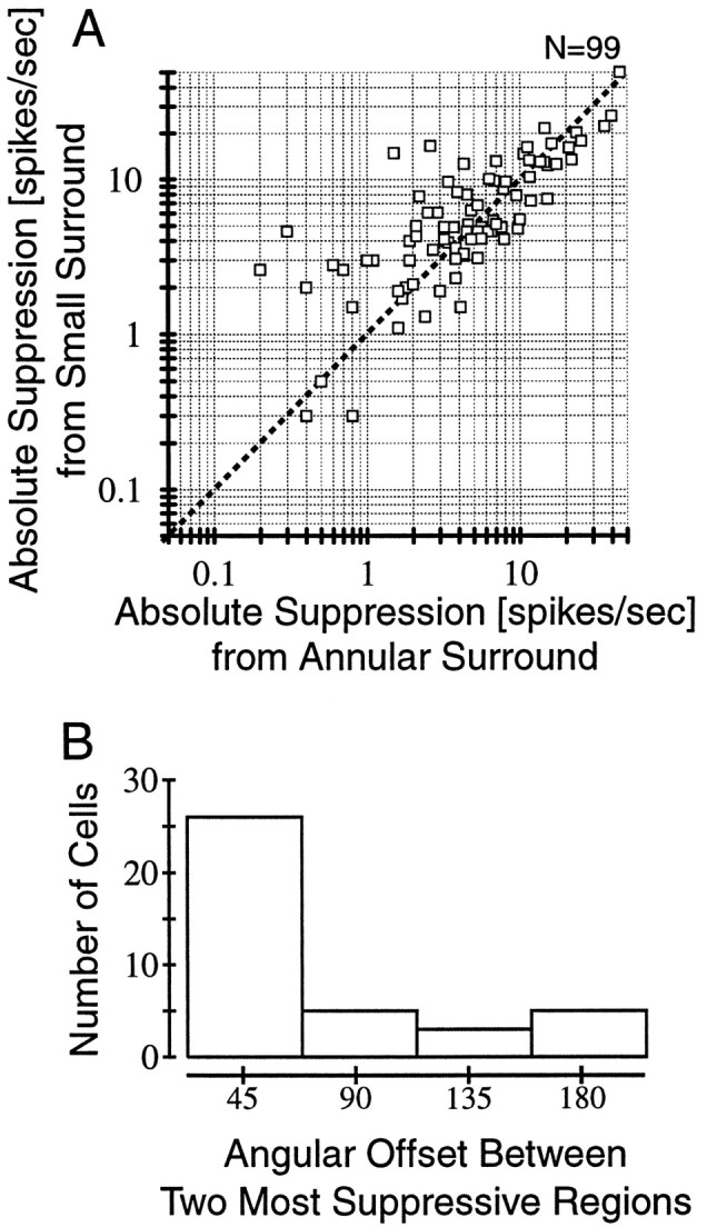
Comparison of the amount of suppression generated by an annular surround stimulus compared with the single most suppressive surround region measured with small grating patches.A, The maximum suppression obtained from one of the eight surround locations is plotted on the x-axis, and the overall (i.e., annular) suppression is plotted on they-axis. Suppression is computed as the absolute spike response rate subtracted from the response obtained with an optimal center stimulus alone. There is a strong and significant (p < 0.0001) correlation (r = 0.83) between the two values. Thus, for most cells, the effect of stimulating the entire surround is matched by a single surround location. B, Typically, suppression is observed at more than one surround location. How far apart are the two most suppressive regions? If suppression is localized, the two most suppressive regions should be adjacent. If suppression is axially symmetric, the next most suppressive region should be 180° away. The histogram in B indicates that the two most suppressive regions were almost always adjacent.

Fig. 10.

Data are shown from a rare example in which the orthogonal surround patch was effective at suppressing the response. InA, strong suppression occurs at the top position and the two adjacent oblique regions. Annulus suppression is 100%. InB, the orthogonal surround provides strong suppression with the annulus (50.4%), and the spatial pattern of asymmetry closely resembles the pattern in A. E, End;S, side.

An analogous and perhaps more intuitive way to think about the SI values is as follows. Consider the modulation of suppression as a harmonic process that changes strength sinusoidally around the circumference of the CRF. Then, one can compute the discrete Fourier transform of surround suppression as it varies around the CRF. SI₁ and SI₂ are equivalent to the amplitude of the fundamental and second harmonic frequency components, respectively. The phase of these harmonics is equivalent to the vector angle computed in Equation 2. We occasionally computed some higher harmonics and determined that they were negligible. Thus, only the first two harmonics are used.

Oblique suppression

In addition to cells that exhibit suppression from the ends and sides of the CRF (Fig. 2), many cells have suppressive regions located intermediately between the ends and sides. We call these regions oblique relative to the preferred orientation axis, and Figure3 shows three examples of this type of suppression. The cell in Figure 3A exhibits clear suppression from one end and an adjacent oblique region. Neither of these regions produces as much suppression as the annular surround, and yet none of the other regions exhibits any substantial inhibition. This implies that the suppressive zone is concentrated in a region spanning portions of the end and the oblique regions, allowing stimuli at both of those positions to partially activate inhibition, but for neither to activate the entire suppressive region. Similar results are shown for the other two cells in Figure 3. Note that the simple cell shown in Figure 3C exhibits only moderate overall suppression (29.53%), but the response reduction is most clear with stimulation of a single oblique region.

Fig. 3.

Three examples of suppression from oblique regions of the surround. A, Simple cell with asymmetrical suppression from an oblique region. This plot was obtained with the surround grating drifting in the opposite direction, although a similar plot was obtained with the same direction in the surround.B, Simple cell exhibiting near complete suppression from one side and one oblique area. C, Complex cell with suppression from an oblique region. There is also some suppression from the adjacent end (E) and side (S) regions, but no other surround position causes any modulation of the baseline response of the cell. In this example, it is also easy to see that the surround-only control conditions do not generate any responses that are significantly different from the ongoing spontaneous activity (innermost circle) of the cell.

Another example of suppression arising from an oblique region is shown for a simple cell in Figure4A. This cell shows strong suppression overall and a large asymmetry when probed with the small surround patches. The plot indicates that the suppressive surround zone for this cell is localized and yet is still larger than the small surround patches, because there is intermediate suppression at several adjacent locations in the surround.

Fig. 4.

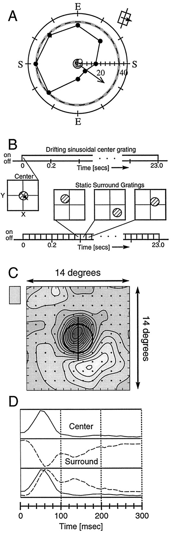
Detailed mapping of oblique surround suppression.A, Another example of suppression arising from an oblique region of the surround, plotted in the same format as Figures 2and 3. E, End; S, side. B, Diagram illustrating the modified reverse correlation method used to obtain a map of the CRF and the suppressive surround. An optimal drifting (conditioning) grating is displayed on one monitor for the duration of the entire block of stimuli (23 sec). During this time, stationary square wave gratings (probe) are presented for 39.5 msec on the other CRT monitor and optically superimposed with the optimal stimulus. The spatial position for each probe grating presentation is randomly chosen from 144 grid locations covering the entire CRF and surround. The spatial phase of the stationary grating is randomly chosen from one of four phases that are multiples of 90°. After all 576 stimuli (144 × 4) have been presented, there is a period of ∼3 sec in which data are stored to a file and the next presentation sequence queued. This process is repeated 100 times. The baseline response from the cell is measured every fifth trial during which the optimal grating is presented alone, without the stationary flashed gratings (these conditions did not count toward the 100 repetitions). The data are processed using our standard reverse correlation analysis software. C, Contour map of the CRF and surround obtained through the modified reverse correlation protocol. The optimal drifting grating in the center measured 4° diameter, indicated by the thick solid circle. The probe grating patch measured 5° in diameter. The 144 grid locations are indicated by the dots in the plot. Darker shading reflects spike rates higher than the maintained discharge, and lighter regions denote regions in which the probe stimulus attenuated the response. D, Average temporal response pattern from the contour map in C, taken at different spatial locations. The top trace is the average temporal response pattern from the CRF. The middle trace is the average response pattern from the suppressive zone (containing points within the fourth contour of the suppressive zone). This curve is smaller in amplitude than the center response and is normalized to facilitate comparisons with the center. The bottom panel compares the temporal responses of the center and suppressive surround, with the trace from the suppressive zone inverted. These traces show that the surround suppression peaks within 10–20 msec of the excitatory center but is more sustained than the center. Additionally, a small secondary peak occurs ∼70 msec after the first peak.

Reverse correlation used to map the surround

One goal of this study is to assess the full two-dimensional shape and size of the surround. To do this, we modified our standard reverse correlation procedure (Freeman and Ohzawa, 1990; DeAngelis et al., 1993) to allow us to simultaneously map the excitatory CRF center and suppressive surround, as illustrated in Figure 4B. A drifting grating of optimal parameters is presented within the CRF for 23 sec to generate an ongoing response. During this time, a second stationary grating patch is presented briefly (39.5 msec), centered at one of 144 grid locations covering both the center and the surround. Because the flashed grating patch is stationary, four different spatial phases are used so that the relative phase differences between the stationary surround grating and drifting central grating cancel out over repeated presentations. We then use the reverse correlation method (Eggermont et al., 1983; Jones and Palmer, 1987; DeAngelis et al., 1993; Ringach et al., 1997) to analyze the responses. One hundred repetitions are completed for each phase and position, and the responses to the four phases are summed to create the smooth-contour plot shown in Figure 4C, which gives a detailed picture of the spatial relationship between the central excitatory region and the suppressive surround zone. On separate trials, the optimal center grating is presented alone to establish the baseline response level of the cell (indicated by the medium gray value shown in thebox adjacent to the plot). In Figure 4C thecircle with the vertical line through it demarcates the spatial area in which the optimal center grating was presented. Spatial regions that caused the cell to respond more strongly than the baseline level are shown in darker shadesof gray, whereas regions that reduced the response of the cell below baseline rate are shown with lighter shades ofgray. The map shows that although most of the surround does not alter the ongoing response, when the area to the bottom right of the CRF is stimulated, the ongoing response is diminished. This conforms precisely to the plot obtained with drifting gratings, as shown in Figure 4A, indicating that the suppressive region is asymmetric. In Figure 4C, it is also apparent that the surround covers an area slightly larger than the CRF and appears to be slightly overlapped with it. Because of the size of the stationary patches, stimuli centered just outside the CRF in most regions still elevate the response, whereas stimuli centered near the border of the CRF and the suppressive region tend to cancel out, causing the CRF to appear to be slightly off center.

Time course of surround suppression

In addition to the spatial information, the map in Figure4C also contains temporal response details that can be extracted by examining the map at different correlation time delays (DeAngelis et al., 1993). The temporal profiles for the center and surround regions have been normalized to facilitate comparisons and are shown in Figure 4D. The top trace is the average temporal response from the spatial region overlapping the CRF. There is a short latency before response onset (∼20 msec) and then a sharp rise leading to a peak response near 50 msec. This is followed by a rapid decrease in response. The middle trace shows the temporal response averaged over the suppressive surround region. Here, there is a decrease in response from the baseline, so the curve has an inverted shape relative to the excitatory response in Figure4D, top. There is a short latency of ∼30 msec and then a sharp decrease from the baseline response. The strongest suppression occurs near 60 msec, but then, unlike the excitatory response, the inhibition does not diminish quickly. The suppression is sustained and remains observable for >150 msec. Curiously, there is another dip in the response that occurs with a latency of ∼130 msec. This dip is weaker than the first but is clearly visible in the trace. It is unclear whether this “bump” has any physiological meaning, but it is tempting to consider that this additional suppression may arise via feedback from extrastriate regions. The latency certainly falls within the range that has been hypothesized in other studies, suggesting that surround suppression originates from higher cortical regions (Lamme, 1995; Zipser et al., 1996).

In Figure 4D, bottom, the surround (inhibitory) trace is inverted and superimposed onto the excitatory response. Note that surround suppression occurs shortly after the excitatory signal, with a relative latency of ∼10 msec. A latency of 10 msec is suggestive of a local mechanism, although it does not rule out feedback from extrastriate or adjacent areas. Nevertheless, the surround effect is clearly evident at 50 msec when the CRF reaches its peak response.

Uniform suppression and axial symmetry

A wide range of spatial patterns of suppression from the surround were observed across the population of cells, although the patterns shown in Figures 2-4 are by far the most common among cells exhibiting surround suppression. At the opposite end of the continuum, a small number of cells gave responses indicative of a uniform, encircling surround. Three of the best examples of uniform surrounds are shown in Figure 5. For these cells, intermediate levels of suppression could be obtained from at least seven of eight surround positions, but no single position produces as much suppression as the entire annulus stimulus. Qualitatively, it appears that there is a pooling of activity from a broad region surrounding the CRF. For these cells, the SI₁ vectors are small, even though the overall suppression can be quite strong when the entire surround is stimulated.

Fig. 5.

Three examples of uniform surround suppression. In all three examples, intermediate levels of suppression are observed from nearly all positions around the center. However, none of the small surround patches produce as much suppression as the annular surround stimulus. Because the suppression is spatially distributed, the SI₁ vector is negligible for each of these cells.E, End; S, side.

Another small group of cells exhibited suppression patterns that were symmetrical. For these cells, suppression is balanced on two opposing regions of the surround. Thus, the suppression is symmetric along one axis. Figure 6Aillustrates an example of this pattern, in which there is no effect when the surround gratings are placed on either side of the CRF, although each end zone produces approximately half of the overall suppression observed with an annular surround stimulus. The SI₁ vector is small because of the axial symmetry of surround of this cell, so in Figure 6A, the SI₂ vector is plotted.

Fig. 6.

Examination of axially symmetric surround suppression. A, Example of a complex cell with axial surround symmetry. Strong suppression was obtained with an annulus covering the entire surround. When probed with small patches, intermediate levels of suppression were obtained from either end (E), and even weaker suppression was obtained from the oblique regions. The sides (S) of the CRF had no influence on the response of the cell. Because of strong axial symmetry, SI₁ is small, so SI₂ is shown in this plot. B, Scatterplot showing the comparison between SI₁ and SI₂ for the population of cells with overall suppression >50% (n = 37). Theunfilled circle denotes the cell shown inA.

One would like to know the proportions of cells in the population that are symmetric or asymmetric. To investigate this question, we compare the magnitude of SI₁ and SI₂. In the extreme case, if a cell is completely asymmetric, SI₁ will be large, and SI₂ will be small. The converse is true if the cell is perfectly symmetrical. Thus, one might expect to find examples of the two extremes as well as intermediate cells. Figure6B plots the magnitude of SI₁versus SI₂ for all cells in the population with >50% surround suppression. We used only cells with strong suppression for this analysis because the SI values can be meaningless as the overall suppression approaches zero. As Figure 6Billustrates, there is a clear continuum of values rather than a dichotomy of two surround patterns.

Localization of surround suppressive zones

As shown above, the surround can be highly asymmetrical, with suppression often arising from a small region. In this section we describe quantitatively the degree of localization. First, a comparison is made between suppression obtained with the small surround patches and the effect of stimulating the entire surround. Then we ask whether there is an organizing principle that governs the regions from which suppression arises. Is there a preference for suppression to originate in a specific portion of the CRF or is it evenly distributed among all surround locations?

If the suppressive regions of the surrounds are restricted to small, localized regions, as the data suggest, then a small grating, properly located, should provide as much suppression as a stimulus covering the entire surround. Alternatively, if the surround contains multiple regions of suppression or is widely distributed around the CRF, the complete annulus should be a more effective inhibitor than any single small surround patch. A third possibility is that the inhibitory surround occupies a large spatial area but exhibits minimal spatial summation. If this is the case, then small surround gratings may stimulate enough of the surround to produce maximal suppression, and we would expect that several surround positions would be able to generate the same degree of suppression as the annulus.

To address these alternatives, the amount of suppression obtained with the single most suppressive surround patch is compared with the effect of stimulating the entire surround (Fig.7A). A strong correlation (r = 0.83; p < 0.0001) is found between the suppression induced by the annulus and the single most effective surround patch. Thus, for many cells, a small surround region can be as effective as the entire surround in suppressing the response of a neuron. This is consistent with the hypothesis that the suppressive region of the surround is highly localized and has spatial dimensions similar to the CRF.

To rule out the possibility that the suppressive region is distributed over a large area but saturates with small stimuli, the suppression obtained with the two most effective surround locations was compared. There are several interesting questions to ask relating to this issue. First, how near to each other are the two most suppressive regions? Are they adjacent or on opposing regions of the CRF? How similar is the level of suppression generated between the two most suppressive regions in the surround? The histogram in Figure 7B shows the angular distance between the two most suppressive regions of the surround and demonstrates that these regions are typically adjacent. Of course, this is what one expects if there is a single suppressive area. Comparing the strength of suppression at the two most effective positions, suppression falls off by a mean of 35.1%. Between the most suppressive region and the third most effective, the falloff is greater (58.6%), indicating that suppression is highly localized.

As described above and in Figures 2-4 and 6, we find that surround asymmetry arises from a variety of positions around the CRF. The question remains whether there is an organizing principle that can describe the location of suppressive surround regions across the population of cells. To address this question, we examined the relative and absolute positions of the suppressive surround zones across the population of cells. Recall that the magnitude of the SI vectors (SI₁ and SI₂) describes the degree of asymmetry observed at the different surround locations and axes. The angles of the SI vectors indicate the interpolated location that produces the strongest suppression, as described in Equation 2. Figure 8 plots an SI value for each cell in our population that satisfies two criteria. First, only the cells that were examined with all eight surround locations are included. Second, the data are limited to those cells that exhibit at least 30% suppression with the annular stimulus. Thirty percent is an arbitrary cutoff value that allows inclusion of the majority of cells but also ensures reasonable signal-to-noise ratio. Finally, the larger of the two SI vectors is used for each cell (Fig. 8, filled andunfilled symbols denote SI₁ and SI₂, respectively), and because SI₂ indicates an axis instead of a single direction, two points, 180° apart, are plotted for each SI₂ vector. Figure 8A plots the position of the suppressive surround relative to the preferred orientation of the cells, such that every data point is rotated so that the preferred orientation of each cell is vertical (consistent with all the sample plots in the previous figures). Thus, a data point lying along the horizontal axis indicates an asymmetric suppression that is strongest from the side of the CRF. The distance of the point from the origin is determined by the SI value and indicates greater asymmetry with greater distance from the origin.

Fig. 8.

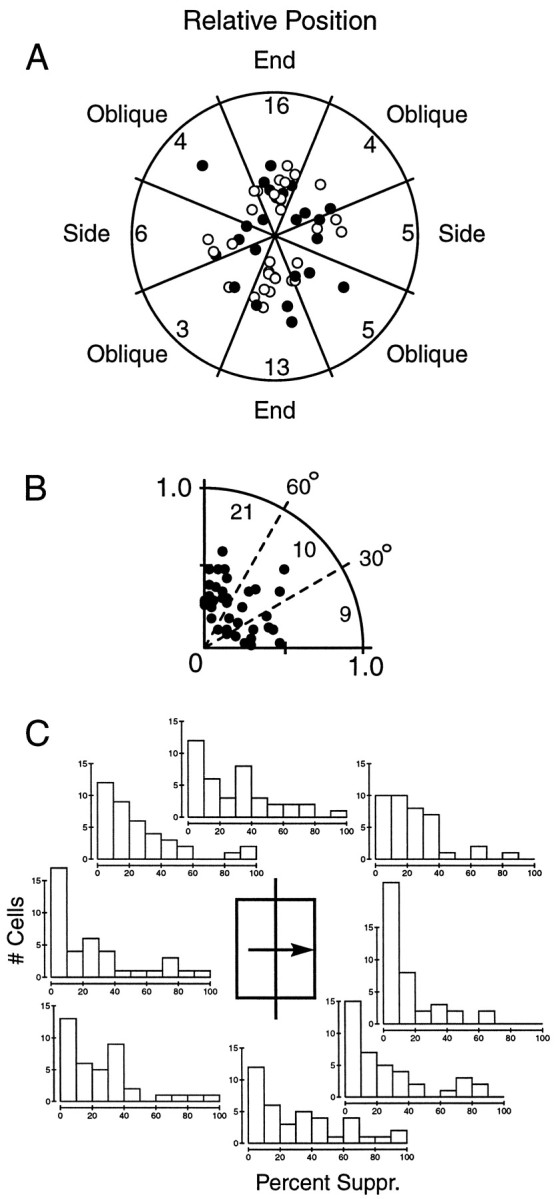
Summary of the spatial regions producing surround suppression. A, This polar plot represents the distribution of suppressive regions from all cells that displayed at least 30% suppression with an annulus stimulus and were measured with eight surround locations (n = 40). Each data point represents an SI vector from an individual cell. The origin represents SI = 0.0, and the outer edge represents SI = 1.0. Thefilled and unfilled circles are the end points of SI₁ (n = 24) and SI₂ (n = 16) vectors, respectively. Because the SI₂ vector indicates an axis rather than a single location, we have plotted two points for each SI₂vector, one along each direction of the axis. The angular position of each point represents the location of the suppressive zone, relative to the preferred orientation of the cell, which has been aligned to vertical for all cells in this plot. The numbers in each sector indicate the numbers of cells that displayed their strongest suppression in that location. Although more cells exhibited suppression from along the end zones, the data do not statistically deviate from a uniform distribution. B, We folded the axes so that all the data in A lie in the first quadrant. Only one point was included for the SI₂cells. We then divided this quadrant into three equal regions subtending 30°. The distribution is dispersed but shows that suppression is approximately twice as likely to originate from an end zone as opposed to an oblique or side zone.

The scatter of data points does not suggest any obvious organizing principle for the spatial distribution of surround suppression, although there are more cells with suppression from the end zone sectors than any of the other sectors. To examine this more closely, the axes of the plot were folded so that all the data lie in the first quadrant and the duplicate data points from the SI₂ vectors are discarded. The results, shown in Figure 8B, exhibit considerable scatter, although approximately half (21 of 40) of all cells lie within 30° of the end axis.

Figure 8, A and B, summarizes the regions of maximal suppression across the population and leads us to two important conclusions. First, the maximal suppression can arise from any location of the surround. Second, there is a slight bias for maximal suppression to arise from the end zones.

Next, we repeated this analysis without rotating the CRFs to vertical (data not shown). In this analysis the surround locations are referenced to a coordinate system on our display monitors outside the animal. We again find no evidence for a systematic organization of suppressive zones, although there is a similar bias for suppression to be located along the horizontal axis (parallel to the ground plane). This finding is intriguing because certain functional advantages can be gained by having suppressive zones offset horizontally. For example,Maske and colleagues (1986) suggest that cells tuned to horizontal could use end stopping to facilitate horizontal disparity detection, to which they would otherwise be insensitive. With our findings of localized suppression occurring at any portion of the surround, any cell with horizontally offset suppression can gain the ability to detect horizontal disparity. Additionally, such suppressive zones can assist in error signals associated with precise vergence eye movements.

Finally, the issue of localization was also examined in another way, by asking the question in a slightly different way. The SI vectors used in the analysis above provided a summary of the suppression for each cell, but in doing so, they reduce the data and discard possibly valuable information. For example, a particular cell might have an SI vector indicating suppression from an oblique region, but this does not inform us whether both the end and oblique regions exhibit suppression or if it is just the oblique area alone. To circumvent this problem, we determined the suppression from each of eight locations in the surround for all cells. The histograms in Figure 8C show the results of this analysis. For clarity, only cells with at least 30% overall suppression and measured with eight surround positions are included. This criterion avoids the inclusion of cells with weak suppression that would obscure the point of this plot, which is to reveal the surround locations that generate meaningful suppression.

For any given surround location, the amount of suppression was usually <20% for all cells in the population. However, for each location, there were also some cells that exhibited nearly complete suppression from that area. These cells were typically the ones that exhibited extreme asymmetries. For any given cell, the suppression at any particular surround location appeared like a random draw from these distributions; most positions showed minimal effects, but usually one or two regions exhibited moderate to strong suppression.

The histograms in Figure 8C are all qualitatively similar, in that they are skewed toward the left. However the two side positions appear somewhat unique, showing a larger number of cells with minimal suppression. For example, 17 and 22 of 40 cells exhibited <10% suppression from the left and right sides of the CRF, respectively.

The data above can be summarized as follows. In most cases, the addition of a small grating in the surround has no effect on the response of a cell unless it is presented in a particular spatial location, and then it usually exerts a purely inhibitory effect. Thus, inhibition is usually only observed when a particular, discrete portion of the surround is stimulated. If the suppressive zone is stimulated, it does not seem to matter if the remainder of the surround is similarly stimulated, so that a small grating in the appropriate place is often as effective as an annulus covering the entire extent of the surround.

Tuning characteristics of the surround suppressive region

Surround suppression is sensitive to stimulus orientation and is typically strongest when the orientation of the surround stimulus matches the preferred orientation of the center (Blakemore and Tobin, 1972; Nelson and Frost, 1978; Knierim and Van Essen, 1992; DeAngelis et al., 1994; Li and Li, 1994; Sillito et al., 1995). There is also evidence that the orientation tuning bandwidth of surround suppression is typically broader than the excitatory bandwidth, so that some cells can exhibit suppression with orthogonally oriented surround stimuli (DeAngelis et al., 1994). Given the asymmetric spatial patterns observed in the surround, we sought to determine whether these patterns are dependent on the orientation of the surround stimulus. In other words, would a given surround region produce suppression if a different orientation was presented in the surround? We also wanted to determine the orientation tuning properties of the surround using small gratings for comparison with data collected using annular surround stimulation.

To examine the basic orientation tuning properties of the surround, the main experiment was repeated using surround gratings oriented 90° (n = 35) or 180° (n = 28) from the preferred orientation of the CRF. An orientation difference of 180° is the same as optimal but opposite in direction of drift.

The majority of cells exhibited surround suppression patterns resembling the two complex cells shown in Figure9. Clear surround suppression is apparent when the center and surround gratings are matched to the preferred orientation and the suppression pattern exhibits spatial asymmetry (Fig. 9A,D). The cell in Figure9A–C illustrates the effect of orientation changes on surround suppression and also provides another example of axially symmetric suppression (Note that SI₂ vector has been plotted for this cell because SI₁ is negligible.) For this cell, the suppression arises from both ends, whereas the side zones have no effect on the response of the cell. The cell in Figure 9D–F exhibits highly asymmetric suppression that originates primarily from one end. For both cells, when the orientation of the surround grating is made orthogonal, the overall suppression is greatly reduced (Fig. 9B,E). Moreover, the spatial pattern of suppression is unclear. Finally, when the surround grating is drifted in the opposite direction, the suppression is comparable with the first condition, and the spatial pattern of suppression is also closely matched. In fact, for these two cells, the asymmetry is marginally stronger in this condition, compared with the iso-direction condition. Note that the SI vectors in the topand bottom plots are equivalent.

Fig. 9.

Suppression patterns with nonoptimal surround stimuli for two complex cells. The grating diagrams at theright of the polar plots indicate the orientation relationship between the central and surround gratings. The central grating is always oriented optimally, and the orientation of the surround grating was either optimal (drifted in the same or opposite direction as the center) or orthogonal. The cell in A–Cexhibits axially symmetry suppression. Accordingly, SI₁ for this cell is small, so we have plotted SI₂. InD–F, SI₁ vectors are plotted. Top row (A, D), The center and surround gratings are matched at the preferred orientation and direction. Suppression is evident from both ends (E) in Aand is absent from either side (S) position. InD, strong suppression is observed only from the bottom end. The annulus suppression is 60.3 and 100% in A andD, respectively. Middle row (B, E), The surround is oriented orthogonally to the central (optimal) grating. The suppression from the annulus and the individual surround gratings is much weaker in B andE with this configuration. The annulus suppression is 33.5 and 36.4% in B and E, respectively.Bottom row (C, F), The surround grating is oriented optimally but is drifted in the opposite (i.e., nonpreferred) direction to that of the center. In C, the pattern of suppression is the same as in A, in which suppression arises from both ends and is absent from the sides. Moreover, the suppression from the annular surround and from the smaller surround patches is slightly stronger than was present inA. The plot in F exhibits the same pattern as in D. The suppression from the annulus is 81.4 and 84% for C and F, respectively.

The two cells shown in Figure 9 are representative of the majority of cells, in which minimal suppression was observed when the surround was orthogonal to the preferred orientation of the CRF, although a few cells did display strong suppression in the orthogonal orientation condition. Figure 10, A andB, shows an example of a cell with strong suppression for both isogonal and orthogonal stimuli in the surround (measurements were not performed with the surround moving in the opposite direction). Although the overall suppression is weaker with orthogonally oriented surround gratings, moderate suppression is observed, and the SI₁ vectors point to locations within 4° of each other for both isogonal and orthogonal orientation conditions. Qualitatively, the spatial patterns of suppression are also closely related. As a general rule, we observed that if strong suppression is found using more than one orientation in the surround, the spatial patterns are always similar to one another.

Altogether, 42 cells were examined with nonoptimal surround gratings in addition to the optimal surround condition. Thirty-five were tested with orthogonal gratings and 28 with gratings moving in the opposite, nonpreferred, direction. Twenty-one of these cells were tested with all three orientation configurations. The results of these experiments are summarized in Figure 11. Thefilled symbols compare the suppression obtained with the isogonally and orthogonally oriented surround. The unfilled symbols compare the suppression observed with iso- and opposite-direction surround stimuli. The two half-filled symbols represent the two cells shown in Figure 9. To simplify the comparison, the percent suppression from the annular surround is used as the metric.

Fig. 11.

Effect of varying orientation of the surround stimulus shown for a subpopulation of 42 cells. The percent suppression is defined as the relative change in response between the optimal center stimulus alone and the optimal center stimulus plus surround annulus. The percent suppression can have a negative value if the addition of the surround annulus causes an increase in response relative to the optimal center stimulus alone. Thex-axis indicates the percent suppression when the center and surround gratings are both set to the preferred value. They-axis is the suppression with optimal center stimulus and nonoptimal surround stimulus. The filled symbols(n = 35) indicate the suppression obtained with orthogonal surround gratings, and the unfilled symbols(n = 28) are conditions in which the surround grating was drifted in the opposite (nonpreferred) direction. The twohalf-filled circles near the top rightindicate the two cells shown in Figure 9. For 21 cells, all three conditions were recorded, and the corresponding data points are connected by vertical lines. Of these, seven are overlapping on the plot. The histogram at the top shows the distribution of the percentage suppression obtained with the optimal orientation used in the surround for the 42 cells shown in the scatterplot. This histogram illustrates the spread of suppression that was typical in this experiment. The histogram on theright illustrates the distribution observed when the surround grating was nonoptimal.

If suppression is independent of the orientation of the surround stimulus, the data should fall on the diagonal 1:1 line. However, most of the data lie below the diagonal line, indicating that surround suppression is strongest with an optimally oriented surround stimulus. A few points do lie above the diagonal line, though, signifying that the overall suppression for these cells is strongest with a nonoptimal surround stimulus. In these cases, the most dramatic effects were usually found with the surround grating drifting in the opposite direction, as illustrated in Figure 9A–C.

For each of the 21 cells that were tested with all three surround configurations, there are two data points displayed in Figure 11. These points have the same x-axis value (suppression with optimal surround) but differ in their y-axis value (suppression with nonoptimal surround). For 7 of these 21 cells, the difference between the two nonoptimal surround orientations is negligible, and the points lie nearly on top of one another. For the other 14 cells, avertical line connects the two points. Among these cells with discernable differences, 10 of 14 display stronger suppression with the opposite direction of drift, compared with the orthogonal grating. Only 6 of 42 cells exhibit their strongest suppression with nonoptimal stimuli.

Finally, the tuning properities of the surround suppression were examined in a more thorough way for two cells with strong suppression and clear asymmetry. The CRF was stimulated with an optimal grating, and a second patch was placed in the portion of the surround that was shown to provide suppression. We then varied the orientation, spatial frequency, and contrast of the surround grating over a broad range of values to explore the surround tuning characteristics. For both cells, as shown in Figure 12, the orientation and spatial frequency tuning appeared as approximately inverted versions of the excitatory tuning from the CRF. The strongest suppression occurred when the orientation and spatial frequency matched the preferred values for the CRF. Surround suppression also increased monotonically with increased surround contrast. Notice that for the cell shown in Figure 12D–F, tuning curves for spatial frequency and contrast were obtained through both eyes, and the results are similar for each eye.

Fig. 12.

Tuning properties of suppressive surround zones for two cells. A, D, The orientation tuning of the CRF is shown in the top trace. The complex cell in A responded maximally to an orientation of 331° but also exhibits a strong response to a grating drifting in the opposite direction (orientation, 151°). A surround orientation tuning (bottom trace) was obtained by placing an optimal grating in the center and a second patch in the region that generated the strongest surround suppression (this relationship is schematized by the gratings at the top). The diamondsare data from three separate surround asymmetry mapping experiments and indicate the response to the optimal center stimulus and the surround annulus at the orientation specified. The response is suppressed to spontaneous levels (<SA) when the surround grating is oriented at 331°. As the orientation of the surround grating deviates from optimal, the suppression decreases and is slightly greater thanRopt (the response to the optimal center stimulus alone) at orthogonal orientations. Suppression is also obtained when the surround grating is oriented 180° from optimal. The simple cell inD is clearly direction-selective in the CRF and is narrowly tuned for orientation. The surround is bidirectional and more broadly tuned, but the strongest suppression matches the preferred orientation of the CRF. B, E, Surround field (SF) tuning of CRF (top trace) and the suppressive surround zone (bottom trace). Again, the peak excitatory SF coincides with the most inhibitory SF for the surround patch, although the inhibitory tuning is broader than the excitatory tuning. In E, responses through both left (circles) and right (squares) eyes were examined. LE and RE denote left and right eyes, respectively. C, F, Contrast response function for the inhibitory surround zone. Suppression increases monotonically with increased contrast of the surround grating. At 30% contrast in the surround, the response was almost completely attenuated. The contrast of the central patch was 35 and 30% for C and F, respectively. The average peak response for the cell in A–C andD–F, is 9.15 and 24.5 spikes/sec, respectively.

The results described above are consistent with previous accounts of tuned surround suppression. However, it is important to note that the present results were obtained using only a small surround stimulus patch placed adjacent to the CRF and not with a large annular surround. Thus, it appears that within the large area surrounding the CRF there is a small suppressive region with tuning similar to the CRF. These results are compatible with the notion that surround suppression originates in cells with similar tuning properties but with spatially displaced CRFs.

“Orientation contrast” has minimal effect on response

Strong response facilitation with surround stimulation has been reported recently (Sillito et al., 1995). In that study, nonoptimal stimuli were presented within the CRF, and optimal stimuli were placed in the surround. For this condition, strong responses were obtained. We attempted to replicate these results. An orthogonally oriented grating was placed in the CRF, and optimally oriented gratings were used to probe the surround in the same manner as in our other experiments. The responses for 31 cells can be summarized by two main observations. First, for most neurons, response to this configuration was at or below the spontaneous level. Responses below the spontaneous level were presumably attributable to the fact that both the center and surround stimuli were oriented for maximal suppressive effect: this caused cross-orientation suppression from within the CRF (DeAngelis et al., 1992; Walker et al., 1998) and iso-orientation surround suppression. Second, several cells responded at rates greater than the spontaneous activity. However, in all cases, these could be accounted for by particular surround locations that drove the cell when presented in isolation. Our interpretation of this is that the stimuli were not properly aligned on the CRF and portions of the optimally oriented surround stimuli were actually overlapping the CRF. Our results are consistent with those of other recent studies in which similar techniques were used. Data from Kastner et al., (1997) and Sengpiel et al. (1997) show no effect in the cat (see Kastner et al., 1997, their Fig. 4; Sengpiel et al., 1997, their Fig. 6D). Likewise, Knierim and Van Essen (1992) do not report any facilitation in the monkey (see their Figs. 2, 4, 10, 11).

Surround suppression in the lateral geniculate nucleus

In this paper, surround suppression is described in area 17. Similar accounts of suppression have also been reported for higher visual areas in the monkey (for review, see Allman et al., 1985). Surround effects are also known in the retina (McIlwain, 1966). Thus, it appears that modulatory surround fields may be ubiquitous in the organization of visual processing at each successive stage. However, details of this organization remain to be identified. With this in mind, we recorded from neurons in the lateral geniculate nucleus (LGN) with two goals. We sought first to determine whether suppression is exhibited by LGN cells and second to determine the feasibility of using our methods from area 17 to map the center and surround of cells in the LGN. The standard protocol was applied for five LGN cells, and for four of these, a reverse correlation mapping was done of the excitatory center and suppressive surround.

The CRF of LGN cells consists of a concentric center–surround organization in the traditional sense. The traditional center–surround organizations of LGN and retinal ganglion cells are different from the surround suppression we have described for the cortical cells. Specifically, the structure of LGN RFs have been described and widely accepted as a difference-of-Gaussian. The surround is not suppressive to drifting grating stimuli that include both bright and dark bars. When the bright bar is centered about the ON center of a LGN cell (thereby producing excitatory effect), the traditional surround receives the dark stimulus areas, which again are excitatory for the cell. Therefore, the traditional center–surround LGN RF organization does not predict any size tuning; the response will monotonically increase with the patch size and eventually plateau. This is exactly what occurred for two cells. However, this is not what we observe in the size-tuning curves for three cells (Fig.13); therefore, we must conclude that the suppression is from an additional mechanism separate from the standard surround of the traditional center–surround organization. We examined the nonclassical surrounds of these cells to evaluate the degree of asymmetric suppression.

Fig. 13.

Data from three cells recorded during an LGN experiment, in which the area beyond the CRF (including both classical center and surround) was investigated for suppression. Eachcolumn represents one cell. The two cells on theright are both ON-center X cells found in layer A. The cell on the left could not be unambiguously dentified as X or Y. The top row shows the size-tuning curve for each cell. <SA, Suppression to spontaneous levels. Thesecond row shows the space–time reverse correlation map of the RF. In these plots, the solid and dashed contours represent responses to bright and dark stimuli, respectively. The centers appear prominently and are followed temporally by larger regions that correspond to the classical surround. The true spatial extent of this surround is probably much larger than it appears in the map, because the reverse correlation stimuli do not reveal weak portions of the surround well. The third rowshows the map of the CRF and the surround region, obtained with the method described in Figure 4B. The cell on thefar right was not mapped with this method, because it did not exhibit any surround suppression in other trials. Thebottom row is the surround mapping obtained with our standard grating method. The cell on the left exhibits asymmetric suppression. The middle cell shows some axial symmetry, and the one on the right exhibits very weak but uniform suppression. E, End; S, side.

The results from the three cells with surround suppression are shown in Figure 13. The left column illustrates the results from a cell that showed clear asymmetry. The top panel is the size-tuning curve, showing strong suppression when the grating is >3°. It should be noted that the suppression is not attributable to the traditional surround of the classical LGN receptive field. Thesecond panel shows the space–time plot of the receptive field, obtained with a standard reverse correlation method (Cai et al., 1997). The classic center–surround structure is visible, but the surround, although weak, probably extends farther than indicated in this map. The third panel shows the map of the receptive field plus the surrounding regions, obtained with the modified reverse correlation method (see Fig. 4B). The receptive field was stimulated with a 2° drifting grating patch, whereas a 5° patch was briefly flashed at a variety of locations. The map shows that when the second grating fell on regions overlapping the conventional LGN receptive field (including the traditional surround), the response was facilitated, but when the second patch fell on a region directly beyond the “top” end of the receptive field, the response was slightly attenuated. This matches the profile obtained with grating stimuli, shown in the bottom panel.

The cell shown in the Figure 13, middle column, was an ON-center X-cell recorded in layer A. This cell has a weaker surround interaction, but the suppression is clear in the size-tuning curve and in the surround mapping with grating stimuli (bottom panel). Note that the error bars are smaller than the data points. The reverse correlation map (third panel) indicates a more uniform suppression, which appears to be concentrated in two regions that correlate well with the grating map (bottom panel). Finally, a cell was also observed that did not show any signs of surround interactions (Fig. 13, right column; ON-center X-cell).

These results, although preliminary, are strongly suggestive. Surround organization outside the CRF of the LGN may be quite similar to that found in the visual cortex. Specifically, there is a suppressive interaction with areas that are beyond the classic center–surround structure. The reverse correlation mapping procedure may provide the best tool for mapping the excitatory and suppressive regions in the LGN, including especially those outside the CRF.

DISCUSSION

Surround suppression throughout the central visual pathway

Based on several independent studies, it appears that surround interactions may be an integral component of receptive field organization throughout the visual pathway. Surround suppression is present in the LGN (Cleland et al., 1983; Jones et al., 1996; our preliminary evidence). Additionally, we find spatial asymmetries that are similar to those found in cortex. From our limited sample, we find that the degree of suppression in the LGN is slightly weaker than that in area 17. This correlates with our observation that the weakest cortical suppression is observed in layer 4 (Walker et al., 1999). Perhaps surround suppression observed in the input layers of the cortex is derived directly from the LGN, whereas intracortical interactions enhance surround effects in other layers. Alternatively, surround suppression in the LGN may result from corticofugal feedback. One could test this by examining the orientation tuning of surround suppression in the LGN. If it is tuned, one may conclude that suppression arises via cortical feedback, whereas untuned suppression would favor a local mechanism derived within the LGN.

Surround asymmetries have also been demonstrated for cells in the MT area of the macaque, and the spatial aspects of these asymmetries appear to be nearly identical to those we report here (Raiguel et al., 1995; Xiao et al., 1995, 1997a,b) (but see Tanaka et al., 1986, who reported symmetrical surrounds in 15 cells tested in MT). Although there are several similarities between the surround organizations in V1 and MT, it is likely that surrounds in MT are created de novo rather than being derived from V1-type input. First, in area MT, nearly all cells are direction-selective (Dubner and Zeki, 1971; Zeki, 1974; Baker et al., 1981; Maunsell and Van Essen, 1983; Albright, 1984; Merigan and Maunsell, 1993), and it has been observed that the surrounds are also direction-selective (Allman et al., 1985). The strongest suppression usually occurs when stimuli in the surround move in the same direction as in the center. When the surround moves in the opposite direction from the center, the responses are often facilitated (Allman et al., 1985; Tanaka et al., 1986). In contrast, we often observe bidirectional suppression in area 17. Second, MT receptive fields are larger than V1, so it is unlikely that the surrounds in MT are built up from V1 surrounds. Recently,Bradley and Andersen (1998) found that many surrounds in MT are also disparity tuned, providing even greater specificity of suppression.

Thus it seems more plausible to presume that the surrounds in any particular region of the brain are locally wired and involve neighboring cells with similar tuning properties. This leads us to ask whether surround interactions occur in other visual areas and, if so, whether they share properties unique to that region. It may turn out that surround interactions are a basic feature of local circuitry at all stages of visual processing. Alternatively, perhaps it is present only in specific areas to facilitate particular types of visual processing.

Functional implications of asymmetrical surrounds

Despite detailed investigation of surround suppression over the years, its functional utility remains unresolved. Several theories have been proposed, although none has been unequivocally proven. One proposal is that end stopping could provide a means of detecting the termination of a line segment (Julesz, 1981, 1984). A similar suggestion is that surround suppression along the length axis could be used to detect curvature (Dobbins et al., 1987, 1989). It is true that a receptive field with inhibitory surround fields on the ends will respond stronger to a “T” junction or a sharply curved line segment compared with an extended straight line. However, the response of such a cell would be undistinguishable from a short straight line entirely within the receptive field. Moreover, cells with oblique or side suppression such as those illustrated in our current paper would be poor detectors of curvature or line termination.

Another idea is that end stopping could lead to the perception of illusory contours (Peterhans and von der Heydt, 1989; von der Heydt and Peterhans, 1989). However, this proposal also uses end inhibition exclusively and ignores suppression from other surround areas. Considering the remarkable tuning and spatial properties of surround suppression, it seems unlikely that its function would be solely to provide a percept of lines that are not even real.

Perhaps the suppressive zones are not specific to the ends or sides but are organized with respect to their position in the visual field. Specifically, we considered the possibility that suppressive zones may be preferentially offset horizontally from the CRF irrespective of the orientation of the cell. Thus, the location of the suppressive region would vary depending on the orientation of the receptive field in space. If the cell prefers vertical stimuli, the suppression would be offset to the side of the receptive field. If horizontal stimuli are preferred, the suppressive zones will be offset to the end of the receptive field. The advantage of this scheme is that surround-suppressed cells could help guide vergence eye movements. Horizontally offset suppressive zones would also assist in detecting depth discontinuities such as those that occur with occluded objects (Maske et al., 1986). Although this theory is appealing, there is no clear trend in the data to support this assertion.

In summary, we find no apparent organizing principle to describe the position of the asymmetrical suppression, although there is a slight bias toward the end zones (Fig. 8). However, this bias is not strong enough to support the assumption that surround effects are predominantly end-based. On the contrary, there is sufficient evidence that surround suppression can arise from any portion of the surround. Therefore, any model that tries to explain or use surround suppression should account for a wide variety of spatial patterns. Thus, we suggest that although the surrounds may indeed lead to the percept of illusory contours, line terminations, or curvature in certain conditions, these features are not likely to be the primary functional utility of the surrounds, and these models need to be reevaluated.

Orientation contrast, figure ground, and pop-out

As demonstrated by our results, a model of surround function should not be tied to the end zones exclusively, but should allow many variations in surround profile. One promising theory posits that the surrounds facilitate our ability to discriminate figures and objects from the backgrounds of visual images. For example, it has been noted that cells often respond to orientation contrast configurations (e.g., a different orientation in the CRF and surround) in a way that correlates with the figure–ground context of the stimulus (Lamme, 1995; Zipser et al., 1996). This has also been related to thepop-out phenomenon in which a particular stimulus appears more salient than the rest of the image (Neisser, 1963; Egeth et al., 1972; Bergen and Julesz, 1983; Treisman and Gormican, 1988). The pop-out phenomenon has been investigated by a number of laboratories, and surround suppression has been suggested as the possible neural substrate for this effect (Nothdurft, 1991; Knierim and Van Essen, 1992; Lamme, 1995; Kastner et al., 1997). Lamme and colleagues (Lamme, 1995; Zipser et al., 1996) go on to suggest that the figure–ground context of a stimulus is determined in extrastriate cortex, which then back-propagates the information to the primary visual cortex, where it helps shape the response of individual cells.

Although the figure–ground theory is attractive, if we examine the basic properties of surround suppression, we find that there is no explicit necessity for the context to be determined by a high-level process. Instead, the very nature of tuned surround suppression could provide the substrate for such a process. For example, surround suppression is typically strongest when the orientation of the center and surround stimuli are both set to the same preferred orientation and usually diminishes as the orientation of the surround grating deviates from the orientation of the central grating (Figs. 9-12). Indeed, we commonly observe that the weakest suppression is obtained when the surround grating is orthogonally oriented. (Figs.9B,E, 11, 12). If we consider the data in a complementary way and examine the response instead of the suppression, we find that the response is greater when an orthogonally oriented grating surrounds an optimally oriented central grating than when an optimally oriented grating is extended to full field. This response property correlates well with the figure–ground context of the image.

This former stimulus described above is referred to as having orientation contrast because there is a difference or contrast between the center and surround orientations. Recently Sillito et al. (1995)reported that certain cells responded strongly to an orientation contrast stimulus, irrespective of the orientation of the central grating. As stated in Results, we did not observe any response when the central stimulus was orthogonal to the optimal and the surround was optimal.

To conclude, notions regarding the functional utility of surround suppression need to be reevaluated in light of our current results. The surrounds are more spatially diverse than previously realized, and we suggest that the surrounds are a consequence of local connections, not high-level feedback, although they may form the basis of high-level operations such as figure–ground discrimination.

REFERENCES

- 1.Albright T. Direction and orientation selectivity of neurons in visual area MT of the macaque. J Neurophysiol. 1984;52:1106–1130. doi: 10.1152/jn.1984.52.6.1106. [DOI] [PubMed] [Google Scholar]
- 2.Albus K, Fries W. Inhibitory sidebands of complex receptive fields in the cats striate cortex. Vision Res. 1980;20:369–372. doi: 10.1016/0042-6989(80)90024-3. [DOI] [PubMed] [Google Scholar]
- 3.Allman J, Miezin F, McGuinness E. Stimulus specific responses from beyond the classical receptive field: Neurophysiological mechanisms for local-global comparisons in visual neurons. Annu Rev Neurosci. 1985;8:407–430. doi: 10.1146/annurev.ne.08.030185.002203. [DOI] [PubMed] [Google Scholar]
- 4.Anzai A, Ohzawa I, Freeman RD. Neural mechanisms underlying binocular fusion and stereopsis: position vs. phase. Proc Natl Acad Sci USA. 1997;94:5438–5443. doi: 10.1073/pnas.94.10.5438. [DOI] [PMC free article] [PubMed] [Google Scholar]
- 5.Baker JF, Petersen SE, Newsome WT, Allman JM. Visual response properties of neurons in four extrastriate visual areas of the owl monkey (Aotus trivirgatus): a quantitative comparison of medial, dorsomedial, dorsolateral, and middle temporal areas. J Neurophysiol. 1981;45:397–416. doi: 10.1152/jn.1981.45.3.397. [DOI] [PubMed] [Google Scholar]
- 6.Batschelet E. Circular statistics in biology. Academic; New York: 1981. [Google Scholar]
- 7.Bergen JR, Julesz B. Parallel versus serial processing in rapid pattern discrimination. Nature. 1983;303:696–698. doi: 10.1038/303696a0. [DOI] [PubMed] [Google Scholar]
- 8.Bishop PO, Kozak W, Vakkur GJ. Some quantitative aspects of the cat's eye: axis and plane of references, visual field co-ordinates and optics. J Physiol (Lond) 1962;163:466–502. doi: 10.1113/jphysiol.1962.sp006990. [DOI] [PMC free article] [PubMed] [Google Scholar]
- 9.Blakemore C, Tobin EA. Lateral inhibition between orientation detectors in the cat's visual cortex. Exp Brain Res. 1972;15:439–440. doi: 10.1007/BF00234129. [DOI] [PubMed] [Google Scholar]
- 10.Bolz J, Gilbert CD. Generation of end-inhibition in the visual cortex via interlaminar connections. Nature. 1986;320:362–365. doi: 10.1038/320362a0. [DOI] [PubMed] [Google Scholar]
- 11.Born RT, Tootell RB. Single-unit and 2-deoxyglucose studies of side inhibition in macaque striate cortex. Proc Natl Acad Sci USA. 1991;88:7071–7075. doi: 10.1073/pnas.88.16.7071. [DOI] [PMC free article] [PubMed] [Google Scholar]
- 12.Bradley DC, Andersen RA. Center-surround antagonism based on disparity in primate area MT. J Neurosci. 1998;18:7552–7565. doi: 10.1523/JNEUROSCI.18-18-07552.1998. [DOI] [PMC free article] [PubMed] [Google Scholar]
- 13.Cai D, DeAngelis GC, Freeman RD. Spatiotemporal receptive field organization in the lateral geniculate nucleus of cats and kittens. J Neurophysiol. 1997;78:1045–1061. doi: 10.1152/jn.1997.78.2.1045. [DOI] [PubMed] [Google Scholar]
- 14.Cleland BG, Lee BB, Vidyasagar TR. Response of neurons in the cat's lateral geniculate nucleus to moving bars of different length. J Neurosci. 1983;3:108–116. doi: 10.1523/JNEUROSCI.03-01-00108.1983. [DOI] [PMC free article] [PubMed] [Google Scholar]
- 15.De Valois RL, Thorell LG, Albrecht DG. Periodicity of striate-cortex-cell receptive fields. J Opt Soc Am A. 1985;2:1115–1123. doi: 10.1364/josaa.2.001115. [DOI] [PubMed] [Google Scholar]
- 16.DeAngelis GC, Robson JG, Ohzawa I, Freeman RD. Organization of suppression in receptive fields of neurons in cat visual cortex. J Neurophysiol. 1992;68:144–163. doi: 10.1152/jn.1992.68.1.144. [DOI] [PubMed] [Google Scholar]
- 17.DeAngelis GC, Ohzawa I, Freeman RD. Spatiotemporal organization of simple-cell receptive fields in the cat's striate cortex. I. General characteristics and postnatal development. J Neurophysiol. 1993;69:1091–1117. doi: 10.1152/jn.1993.69.4.1091. [DOI] [PubMed] [Google Scholar]
- 18.DeAngelis GC, Freeman RD, Ohzawa I. Length and width tuning of neurons in the cat's primary visual cortex. J Neurophysiol. 1994;71:347–374. doi: 10.1152/jn.1994.71.1.347. [DOI] [PubMed] [Google Scholar]
- 19.Dobbins A, Zucker SW, Cynader MS. Endstopped neurons in the visual cortex as a substrate for calculating curvature. Nature. 1987;329:438–441. doi: 10.1038/329438a0. [DOI] [PubMed] [Google Scholar]
- 20.Dobbins A, Zucker SW, Cynader MS. Endstopping and curvature. Vision Res. 1989;29:1371–1387. doi: 10.1016/0042-6989(89)90193-4. [DOI] [PubMed] [Google Scholar]
- 21.Dubner R, Zeki SM. Response properties and receptive fields of cells in an anatomically defined region of the superior temporal sulcus in the monkey. Brain Res. 1971;35:528–532. doi: 10.1016/0006-8993(71)90494-x. [DOI] [PubMed] [Google Scholar]
- 22.Egeth H, Jonides J, Wall S. Parallel processing of multi-element displays. Cognit Psychol. 1972;3:674–698. [Google Scholar]
- 23.Eggermont JJ, Johannesma PIM, Aertsen AMHJ. Reverse-correlation methods in auditory research. Q Rev Biophys. 1983;16:341–414. doi: 10.1017/s0033583500005126. [DOI] [PubMed] [Google Scholar]
- 24.Field DJ, Hayes A, Hess RF. Contour integration by the human visual system: evidence for a local “association field.”. Vision Res. 1993;33:173–193. doi: 10.1016/0042-6989(93)90156-q. [DOI] [PubMed] [Google Scholar]
- 25.Freeman RD, Ohzawa I. On the neurophysiological organization of binocular vision. Vision Res. 1990;30:1661–1676. doi: 10.1016/0042-6989(90)90151-a. [DOI] [PubMed] [Google Scholar]
- 26.Ghose GM, Ohzawa I, Freeman RD. A flexible PC-based physiological monitor for animal experiments. J Neurosci Methods. 1995;62:7–13. doi: 10.1016/0165-0270(95)00048-8. [DOI] [PubMed] [Google Scholar]
- 27.Glezer VD, Ivanoff VA, Tscherbach TA. Investigation of complex and hypercomplex receptive fields of visual cortex of the cat as spatial frequency filters. Vision Res. 1973;13:1875–1904. doi: 10.1016/0042-6989(73)90061-8. [DOI] [PubMed] [Google Scholar]
- 28.Hubel DH, Wiesel TN. Receptive fields, binocular interaction, and functional architecture in the cat's visual cortex. J Physiol (Lond) 1962;160:106–154. doi: 10.1113/jphysiol.1962.sp006837. [DOI] [PMC free article] [PubMed] [Google Scholar]
- 29.Hubel DH, Wiesel TN. Receptive fields and functional architecture in two non-striate visual areas (18 and 19) of the cat. J Neurophysiol. 1965;23:229–289. doi: 10.1152/jn.1965.28.2.229. [DOI] [PubMed] [Google Scholar]
- 30.Jones HE, Cudeiro J, Sillito AM. Context dependent visual processing in lateral geniculate nucleus (LGN) and visual cortex. Invest Ophthalmol Vis Sci [Suppl] 1996;37:1058. [Google Scholar]
- 31.Jones JP, Palmer LA. The two-dimensional spatial structure of simple receptive fields in cat striate cortex. J Neurophysiol. 1987;58:1187–1211. doi: 10.1152/jn.1987.58.6.1187. [DOI] [PubMed] [Google Scholar]
- 32.Julesz B. Textons, the elements of texture perception, and their interactions. Nature. 1981;290:91–97. doi: 10.1038/290091a0. [DOI] [PubMed] [Google Scholar]
- 33.Julesz B. Toward an axiomatic theory of preattentive vision. In: Edelman G, Cowan WM, editors. Dynamic aspects of neocortical function. Wiley; New York: 1984. pp. 585–612. [Google Scholar]
- 34.Kapadia MK, Ito M, Gilbert CD, Westheimer G. Improvement in visual sensitivity by changes in local context: parallel studies in human observers and in V1 of alert monkey. Neuron. 1995;15:843–856. doi: 10.1016/0896-6273(95)90175-2. [DOI] [PubMed] [Google Scholar]
- 35.Kastner S, Nothdurft H-C, Pigarev IN. Neuronal correlates of pop-out in cat striate cortex. Vision Res. 1997;37:371–376. doi: 10.1016/s0042-6989(96)00184-8. [DOI] [PubMed] [Google Scholar]
- 36.Kato H, Bishop PO, Orban GA. Hypercomplex and simple/complex cell classifications in cat striate cortex. J Neurophysiol. 1978;41:1071–1095. doi: 10.1152/jn.1978.41.5.1071. [DOI] [PubMed] [Google Scholar]
- 37.Knierim JJ, Van Essen DC. Neuronal responses to static texture patterns in area V1 of the alert macaque monkey. J Neurophysiol. 1992;67:961–980. doi: 10.1152/jn.1992.67.4.961. [DOI] [PubMed] [Google Scholar]
- 38.Lamme VAF. The neurophysiology of figure–ground segregation in primary visual cortex. J Neurosci. 1995;15:1605–1615. doi: 10.1523/JNEUROSCI.15-02-01605.1995. [DOI] [PMC free article] [PubMed] [Google Scholar]
- 39.Levick WR. Another tungsten microelectrode. Med Biol Eng. 1972;10:510–515. doi: 10.1007/BF02474199. [DOI] [PubMed] [Google Scholar]
- 40.Levitt JB, Lund JS. Contrast dependence of contextual effects in primate visual cortex. Nature. 1997;387:73–76. doi: 10.1038/387073a0. [DOI] [PubMed] [Google Scholar]
- 41.Li C, Li W. Extensive integration field beyond the classical receptive field of cat's striate cortical neurons—classification and tuning properties. Vision Res. 1994;34:2337–2355. doi: 10.1016/0042-6989(94)90280-1. [DOI] [PubMed] [Google Scholar]
- 42.Maffei L, Fiorentini A. The unresponsive regions of visual cortical receptive fields. Vision Res. 1976;16:1131–1139. doi: 10.1016/0042-6989(76)90253-4. [DOI] [PubMed] [Google Scholar]
- 43.Maske R, Yamane S, Bishop PO. End-stopped cells and binocular depth discrimination in the striate cortex of cats. Proc R Soc Lond B Biol Sci. 1986;229:257–276. doi: 10.1098/rspb.1986.0085. [DOI] [PubMed] [Google Scholar]
- 44.Maunsell JH, Van Essen DC. Functional properties of neurons in middle temporal visual area of the macaque monkey. I. Selectivity for stimulus direction, speed, and orientation. J Neurophysiol. 1983;49:1127–1147. doi: 10.1152/jn.1983.49.5.1127. [DOI] [PubMed] [Google Scholar]
- 45.McIlwain JT. Some evidence concerning the physiological basis of the periphery effect in the cat's retina. Exp Brain Res. 1966;1:265–271. doi: 10.1007/BF00234346. [DOI] [PubMed] [Google Scholar]
- 46.Merigan WH, Maunsell JHR. How parallel are the primate visual pathways? Annu Rev Neurosci. 1993;16:369–402. doi: 10.1146/annurev.ne.16.030193.002101. [DOI] [PubMed] [Google Scholar]
- 47.Neisser U. Decision time without reaction time: experiments in visual scanning. Am J Psychol. 1963;76:376–385. [Google Scholar]
- 48.Nelson JI, Frost J. Orientation-selective inhibition from beyond the classic visual receptive field. Brain Res. 1978;139:359–365. doi: 10.1016/0006-8993(78)90937-x. [DOI] [PubMed] [Google Scholar]
- 49.Nothdurft HC. Texture segmentation and pop-out from orientation contrast. Vision Res. 1991;31:1073–1078. doi: 10.1016/0042-6989(91)90211-m. [DOI] [PubMed] [Google Scholar]
- 50.Orban GA, Kato H, Bishop PO. End-zone region in receptive fields of hypercomplex and other striate neurons in the cat. J Neurophysiol. 1979a;42:818–832. doi: 10.1152/jn.1979.42.3.818. [DOI] [PubMed] [Google Scholar]
- 51.Orban GA, Kato H, Bishop PO. Dimensions and properties of end-zone inhibitory areas in receptive fields of hypercomplex cells in cat striate cortex. J Neurophysiol. 1979b;42:833–849. doi: 10.1152/jn.1979.42.3.833. [DOI] [PubMed] [Google Scholar]
- 52.Peterhans E, von der Heydt R. Mechanisms of contour perception in monkey visual cortex. II. Contours bridging gaps. J Neurosci. 1989;9:1749–1763. doi: 10.1523/JNEUROSCI.09-05-01749.1989. [DOI] [PMC free article] [PubMed] [Google Scholar]
- 53.Polat U, Norcia AM. Neurophysiological evidence for contrast dependent long-range facilitation and suppression in the human visual cortex. Vision Res. 1996;36:2099–2109. doi: 10.1016/0042-6989(95)00281-2. [DOI] [PubMed] [Google Scholar]
- 54.Polat U, Sagi D. Lateral interactions between spatial channels: suppression and facilitation revealed by lateral masking experiments. Vision Res. 1993;33:993–999. doi: 10.1016/0042-6989(93)90081-7. [DOI] [PubMed] [Google Scholar]
- 55.Polat U, Sagi D. The architecture of perceptual spatial interactions. Vision Res. 1994;34:73–78. doi: 10.1016/0042-6989(94)90258-5. [DOI] [PubMed] [Google Scholar]
- 56.Polat U, Mizobe K, Pettet MW, Kasamatsu T, Norcia AM. Collinear stimuli regulate visual response depending on cell's contrast threshold. Nature. 1998;391:580–584. doi: 10.1038/35372. [DOI] [PubMed] [Google Scholar]
- 57.Raiguel S, Van Hulle MM, Xiao D-K, Marcar VL, Orban GA. Shape and spatial distribution of receptive fields and antagonistic motion surrounds in the middle temporal area (V5) of the macaque. Eur J Neurosci. 1995;7:2064–2082. doi: 10.1111/j.1460-9568.1995.tb00629.x. [DOI] [PubMed] [Google Scholar]
- 58.Ringach DL, Hawken MJ, Shapley R. Dynamics of orientation tuning in macaque primary visual cortex. Nature. 1997;387:281–284. doi: 10.1038/387281a0. [DOI] [PubMed] [Google Scholar]
- 59.Rose D. Response of single units in cat visual cortex to moving bars of light as a function of bar length. J Physiol (Lond) 1977;271:1–23. doi: 10.1113/jphysiol.1977.sp011987. [DOI] [PMC free article] [PubMed] [Google Scholar]
- 60.Rossi AF, Rittenhouse CD, Paradiso MA. The representation of brightness in primary visual cortex. Science. 1996;273:1104–1107. doi: 10.1126/science.273.5278.1104. [DOI] [PubMed] [Google Scholar]
- 61.Sengpiel F, Sen A, Blakemore C. Characteristics of surround inhibition in cat area 17. Exp Brain Res. 1997;116:216–228. doi: 10.1007/pl00005751. [DOI] [PubMed] [Google Scholar]
- 62.Sillito AM, Grieve KL, Jones HE, Cudeiro J, Davis J. Visual cortical mechanisms detecting focal orientation discontinuities. Nature. 1995;378:492–496. doi: 10.1038/378492a0. [DOI] [PubMed] [Google Scholar]
- 63.Skottun BC, De Valois RL, Grosof DH, Movshon JA, Albrecht DG, Bonds AB. Classifying simple and complex cells on the basis of response modulation. Vision Res. 1991;31:1079–1086. doi: 10.1016/0042-6989(91)90033-2. [DOI] [PubMed] [Google Scholar]
- 64.Stemmler M, Usher M, Niebur E. Lateral interactions in primary visual cortex: a model bridging physiology and psychophysics. Science. 1995;269:1877–1880. doi: 10.1126/science.7569930. [DOI] [PubMed] [Google Scholar]
- 65.Sutter EE. A deterministic approach to nonlinear systems analysis. In: Pinter RB, Nabet B, editors. Nonlinear vision. CRC; Boca Raton, FL: 1992. pp. 171–220. [Google Scholar]
- 66.Tanaka K, Hikosaka K, Saito H, Yukie M, Fukada Y, Iwai E. Analysis of local and wide-field movements in the superior temporal visual areas of the macaque monkey. J Neurosci. 1986;6:134–144. doi: 10.1523/JNEUROSCI.06-01-00134.1986. [DOI] [PMC free article] [PubMed] [Google Scholar]
- 67.Treisman A, Gormican S. Feature analysis in early vision: evidence from search asymmetries. Psychol Rev. 1988;95:15–48. doi: 10.1037/0033-295x.95.1.15. [DOI] [PubMed] [Google Scholar]
- 68.von der Heydt R, Peterhans E. Mechanisms of contour perception in monkey visual cortex. I. Lines of pattern discontinuity. J Neurosci. 1989;9:1731–1748. doi: 10.1523/JNEUROSCI.09-05-01731.1989. [DOI] [PMC free article] [PubMed] [Google Scholar]
- 69.Walker GA, Ohzawa I, Freeman RD. Binocular cross-orientation suppression in the cat's striate cortex. J Neurophysiol. 1998;79:227–239. doi: 10.1152/jn.1998.79.1.227. [DOI] [PubMed] [Google Scholar]
- 70.Walker GA, Ohzawa I, Freeman RD (1999) Surround suppression outside the classical cortical receptive field. Vis Neurosci, in press. [DOI] [PubMed]
- 71.Xiao D-K, Raiguel S, Marcar V, Koenderink J, Orban GA. Spatial heterogeneity of inhibitory surrounds in the middle temporal visual area. Proc Natl Acad Sci USA. 1995;92:11303–11306. doi: 10.1073/pnas.92.24.11303. [DOI] [PMC free article] [PubMed] [Google Scholar]
- 72.Xiao DK, Raiguel S, Marcar V, Orban GA. The spatial distribution of the antagonistic surround of MT/V5 neurons. Cereb Cortex. 1997a;7:662–677. doi: 10.1093/cercor/7.7.662. [DOI] [PubMed] [Google Scholar]
- 73.Xiao D-K, Marear VL, Raiguel SE, Orban GA. Selectivity of macaque MT/V5 neurons for surface orientation in depth specified by motion. Eur J Neurosci. 1997b;9:956–964. doi: 10.1111/j.1460-9568.1997.tb01446.x. [DOI] [PubMed] [Google Scholar]
- 74.Zeki SM. Functional organisation of a visual area in the posterior bank of the superior temporal sulcus of the rhesus monkey. J Physiol (Lond) 1974;236:549–573. doi: 10.1113/jphysiol.1974.sp010452. [DOI] [PMC free article] [PubMed] [Google Scholar]
- 75.Zipser K, Lamme VAF, Schiller PH. Contextual modulation in primary visual cortex. J Neurosci. 1996;16:7376–7389. doi: 10.1523/JNEUROSCI.16-22-07376.1996. [DOI] [PMC free article] [PubMed] [Google Scholar]