Spatial Summation in the Receptive Fields of MT Neurons

Abstract

Receptive fields (RFs) of cells in the middle temporal area (MT or V5) of monkeys will often encompass multiple objects under normal image viewing. We therefore have studied how multiple moving stimuli interact when presented within and near the RF of single MT cells. We used moving Gabor function stimuli, <1° in spatial extent and ∼100 msec in duration, presented on a grid of possible locations over the RF of the cell. Responses to these stimuli were typically robust, and their small spatial and temporal extent allowed detailed mapping of RFs and of interactions between stimuli. The responses to pairs of such stimuli were compared against the responses to the same stimuli presented singly. The responses were substantially less than the sum of the responses to the component stimuli and were well described by a power-law summation model with divisive inhibition. Such divisive inhibition is a key component of recently proposed “normalization” models of cortical physiology and is presumed to arise from lateral interconnections within a region. One open question is whether the normalization occurs only once in primary visual cortex or multiple times in different cortical areas. We addressed this question by exploring the spatial extent over which one stimulus would divide the response to another and found effective normalization from stimuli quite far removed from the RF center. This supports models under which normalization occurs both in MT and in earlier stages.

Extrastriate cortex of monkeys contains a series of linked areas, often termed the “motion system,” which are highly specialized for the analysis of visual motion. The middle temporal area (MT, or V5) appears to take an intermediate position in this hierarchically organized series of areas. One correlate of the hierarchy in this pathway is progressively increasing receptive field (RF) size. Thus, the RFs of MT cells are larger than those of their inputs by as much as a factor of 10 and smaller than those of its targets by a similar ratio (Maunsell and Van Essen, 1983b; Tanaka et al., 1986; Raiguel et al., 1995, 1997; Movshon and Newsome, 1996). Spatial summation is therefore prevalent in extrastriate cortex and is probably important in the function of the motion system. Despite this, few quantitative measurements of summation have been made outside of striate cortex. In this paper, we used small, transient motion stimuli to densely map spatial interactions in MT cell RFs. These were presented individually or pair-wise over the RFs of MT cells. The rapid stimulus sequence allowed us to explore a very large number of combinations of different locations and thus to obtain new and detailed information on the spatial structure of MT cell spatial interactions. This stimulation method might be generally useful for other studies that require the exploration of many stimulus conditions. In our default conditions, we used 300 distinct stimulus conditions for each cell and could gather adequate data in a practical span of time.

Two classes of experiment have described summation in MT, but neither has explored the current question of interactions within and near the RF center. Several experiments have addressed the interaction between the classical RF center and the antagonistic surround (Allman et al., 1985; Born and Tootell, 1992; Raiguel et al., 1995). The surround may overlap with the RF center, but to evaluate this question, we need to know how stimuli interact in the RF center and its immediate neighborhood.

Other studies have measured responses to multiple stimuli moving through the RF of MT cells. The stimuli have either been pairs of dots traversing the RF (Ferrera and Lisberger, 1997; Recanzone et al., 1997) or moving dot fields (Britten and Newsome, 1990; Snowden et al., 1991). The general result from these studies is that MT cellsaverage multiple inputs. In other words, the evoked response when presented with two stimuli together will be intermediate between the responses to each presented alone. This result indicates that linear summation is an inadequate explanation; an additional step is required. A candidate for this extra step is provided by a recent model (Simoncelli and Heeger, 1998) of MT that employs recursive, divisive inhibition to scale the responses of MT cells by an amount proportional to total activity in some region. However, no experiment has addressed the spatial extent of the mutually inhibitory interactions in MT. Our experiment provides the first direct test of the spatial extent of such inhibitory interactions.

These results have previously appeared in abstract form (Britten, 1995).

MATERIALS AND METHODS

Preparation. Two adult female rhesus macaques (Macaca mulatta) were used in this study. Before recording, each had been trained to fixate stationary targets in the presence of visual stimuli. Each was implanted with a scleral search coil (Judge et al., 1980) and was equipped with a stainless steel head restraint post and recording cylinder located over occipital cortex. A plastic grid secured inside this cylinder provided a coordinate system of guide tube support holes at 1 mm intervals (Crist et al., 1988). Animal procedures complied with the Institute for Laboratory Animal Research Guide for the Care and Use of Laboratory Animals and were approved by the University of California Davis Animal Care and Use Committee. On recording days, guide tubes were inserted transdurally through these holes, and Parylene-insulated tungsten microelectrodes were inserted through the guide tubes. To localize area MT, we used both anatomical and physiological landmarks. Anatomical landmarks included recording depth and the transitions between active gray matter and “silent” areas marking white matter or sulci. Physiological landmarks included brisk, directional responses, retinotopy, receptive field size, and columnar organization for preferred direction.

Once MT was localized, we would record and isolate activity using standard extracellular methods. Electrode signals were amplified and filtered, and single spikes were converted to digital pulses, whose time of arrival would be recorded with 1 msec resolution using the public domain software package REX (Hays et al., 1982). Search stimuli were chosen to match local multiunit preferences and could be moving bars, dot fields, or Gabor motion impulse stimuli. Once a cell was isolated, its RF location was crudely mapped using hand-held moving bar stimuli, and quantitative testing commenced.

Stimuli. All stimuli were presented on the face of a cathode ray terminal monitor, subtending 60° horizontally by 48° vertically (1280 × 1024 pixels), operating at a vertical refresh rate of 72 Hz. Stimuli were generated by custom software running on a dedicated display computer. For early experiments, we used an SGI (Mountain View, CA) Indigo2, and in later experiments, we used a Pentium personal computer hosting an ATI Technologies (Thornhill, Ontario, Canada) Mach 64 video card, running in 8 bit mode. Screen luminance was measured as a function of gray scale value using a Tektronix (Wilsonville, OR) photometer, fit with a cubic polynomial, and this was inverted to establish a linearized gray scale lookup table. Average screen luminance was set to 30 cd/M², and maximum achievable contrast was effectively 100% (background luminance was 0.1 cd/M²).

The stimuli for these experiments were moving, two-dimensional oriented “motion impulses,” whose spatial luminance function was a Gabor function, or the product of a sine wave and a Gaussian function. These are members of the family that Watson refers to as “generalized Gabors” (Watson and Turano, 1995), which have the property that both carrier (the sine wave) and the Gaussian contrast envelope are free to move. In our case, carrier and envelope moved together in the preferred direction of the cell under study. One such stimulus is illustrated in Figure 1A. The space–time luminance was described by the function:

$$L(x,y,t)=C(t)\times exp\left[-\frac{(x-{\mu }_x{)}^2}{{\varsigma }_x^2}\right]\times exp\left[-\frac{(y-{\mu }_y{)}^2}{{\varsigma }_y^2}\right]\times sin(\omega x),$$ Equation 1

where (μ_x,μ_y) is the instantaneous location of the center of the impulse, and (ς_x,ς_y) describe its dimensions. The coordinate system is rotated so that the positivex-axis is in the preferred direction of the cell under study. The constant ω establishes the spatial frequency of the carrier. The x coordinate of the center of the impulse moved linearly in time, and the spatial offset per frame was usually set to one-fourth of the cycle of the carrier. The contrast functionC(t) was a trapezoid spanning seven frames (98 msec) illustrated in Figure 1B. The default values for these parameters were 1.07 cycles/deg carrier spatial frequency, 18 Hz temporal frequency, ς_x = 0.56°, and ς_y = 1.12. It is worth noting that the small dimensions of the contrast envelope relative to the underlying carrier frequency made these stimuli spatially rather broad-band, compared with “typical” Gabor stimuli; this was a necessary consequence of their small spatial dimensions. These were adjusted only if the cell responded poorly or if the stimulus grid was so small that adjacent stimulus locations would overlap. We did not attempt to exhaustively search for optimal parameters but inspected on-line raster displays for responses clearly above baseline and listened for stimulus-related modulation on the audio monitor.

Fig. 1.

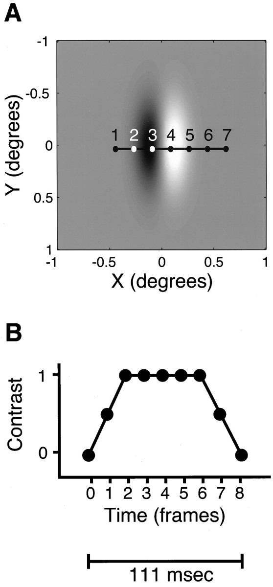
Single Gabor motion impulse depicted as a function of space and time. A, Two-dimensional representation of typical stimulus. This portrays the default values for spatial parameters used in these experiments, which were only varied if these proved ineffective in driving the cell. Aspect ratio was always 2:1, but the ratio of carrier period to Gaussian envelope was more variable. The numbered points indicate the successive locations of an arbitrary spatial reference point in seven successive frames of the stimulus; the white numbers are only for graphic clarity. B, Contrast as a function of time. Eachpoint represents a single frame, corresponding to the locations indicated in A. In a sequence of continuously presented stimuli, the next stimulus frame 0 would immediately follow frame 8, producing an overall interval of 125 msec between successive stimuli.

These stimuli were presented in a rapid sequence, with only two frames intervening between sequentially presented impulses (Fig.1B), and the location of the next impulse(s) was selected pseudorandomly. Single trials consisted of periods ∼3 sec in duration during which the monkey was required to hold fixation during stimulus presentation, and the monkey was rewarded for correctly maintaining fixation. The final individual stimulus period in trials in which fixation was broken was discarded from subsequent analysis.

Locations of the Gabors were chosen from a 5 × 5 grid of possible locations, covering the RF of the cell, illustrated in Figure2. The circle schematically illustrates the RF of the neuron under study, showing that the intended configuration placed the corners of the grid off the RF, in largely unresponsive locations. However, there was substantial random variation in the exact relationship between RF size and grid dimensions, because the hand-mapping stimulus often provided a different estimate of the RF boundary than did the Gabors.

Fig. 2.

Spatial arrangement of Gabor impulses, schematically illustrated over an MT cell RF (circle). Stimuli could either be presented individually or else in pairs (illustrated). The direction of the stimuli (arrows) was adjusted to match the preference of the cell, and the dimensions were adjusted so the corner stimuli gave approximately equal, very small responses.

Two different types of blocks of trials were presented, in which the stimuli were presented singly or in pairs. Each individual stimulus and pair-wise combination (in the paired-stimulus blocks) was presented an equal number of times. Typically, the single-stimulus block was presented first, and inspection of on-line peristimulus time histogram (PSTH) displays would reveal if adjustment of the grid size or location was required. Usually, 50 presentations of each stimulus location were given in the single-stimulus blocks, and for the double-stimulus block, trials were run for as long as the cell could be held. For the data presented in this paper, the number of presentations of each combination of locations ranged from 4 to 151, with a median of 21.

Data analysis. Spike times were extracted from the raw data files, corrected for the vertical location of the stimulus on the screen (the raster was measured to take 12 msec to traverse the vertical extent of the screen), and compiled into standard PSTHs. For calculating spike rates, identical windows of 25–150 msec after stimulus were used for both the single-stimulus and paired-stimulus trials.

For collapsing data across cells, individual cell RF profiles were fit with two-dimensional, oriented Gaussian functions, allowing standardization of different RF profiles to a single “standard” RF. The Gaussian functions to which the single-stimulus data were fit were of the form:

$$R(x^{\prime },y^{\prime })$$ Equation 2

$$=A\times exp\left[-0.5\times \frac{(x^{\prime }-{\mu }_x{)}^2}{{\varsigma }_x^2}\right]\times exp\left[-0.5\times \frac{(y^{\prime }-{\mu }_y{)}^2}{{\varsigma }_y^2}\right]+C,$$

where (x′,y′) are rotated from screen coordinates by an angle θ, A is an amplitude parameter, and C is the maintained activity.

Histology. One of the monkeys used in this study has been killed, and histological confirmation of the recordings was obtained. Before killing, two fluorescent tracer injections were made through the guide tube support grid in known locations. The monkey was killed with an overdose of barbiturates and perfused transcardially with 0.9% saline followed by fixative (4% paraformaldehyde in 0.1m phosphate buffer), followed by fixative with 10% sucrose. The brain was removed, allowed to sink in 30% sucrose solution, and then blocked and parasagitally sectioned at 50 μm thickness on a freezing microtome. Alternate series were stained for myelin (Gallyas, 1979) and for Nissl substance and mounted for fluorescence imaging. The location of the injection sites was charted on the superior temporal sulcus and used to confirm that the recording sites were in the heavily myelinated region corresponding to area MT. The other monkey is alive and being used in other experiments.

RESULTS

We recorded from 89 cells in two hemispheres of two adult female macaques. In 72 of these, we held the cells long enough to measure responses to stimuli presented in pairs. In this section, we first document the responsiveness of the neurons to these stimuli presented singly and then turn to the interactions between pairs.

Single-stimulus responses

These responses came from the blocks of trials in which stimuli were presented singly. Before we consider how these responses vary across the RF, we need to look at the temporal dynamics of the responses. This will allow us to establish appropriate time windows for measuring responses. Figure 3 shows the “grand average” PSTH for all cells and all stimulus conditions. Each individual response (cell and location) was independently normalized, so this shows the average temporal dynamics of the sample as a whole, independent of response amplitude. The figure shows a clear response transient starting ∼30 msec after stimulus onset, rising to peak at 50 msec, and then falling without reaching a clear plateau, as one would expect for longer-duration stimuli. We chose to select one time window for all spike rate analysis, to avoid problems with selection of individual cell response windows, which can be unreliable or subjective. In this figure, the vertical lines show the boundaries of the time window chosen for subsequent analysis.

Fig. 3.

Grand average temporal envelope of MT response to single motion impulses. The responses of each cell were individually normalized and then averaged to produce the histogram shown. Thevertical dashed lines indicate the boundaries of the temporal window used to calculate the rates used as the principal response metric in this paper. The bold horizontal lineabove the histogram denotes the stimulus period. The histogram peaks to which these responses were normalized averaged 102 impulses/sec across our sample of cells, and the average integrated response above baseline, in the center of each RF, was 61 impulses/sec.

We next sought to estimate the dependence of response on location for each cell. Results from two example cells are illustrated in Figure4. For each cell, PSTHs from each of the 25 stimulus locations are shown. These examples are chosen to represent both the range of grid dimensions used, relative to the size of the RF, and the range of cell response magnitudes to these stimuli. Most importantly, in nearly all cases, the range of stimulus locations used in the grid provoked wide response differences from location to location; we thus have sampled the spatial dynamic range of each cell. Although we did not reach the edge of the RF for every cell in the sample, in all we covered enough of the RF to well estimate its shape.

Fig. 4.

Responses of two representative MT cells, shown as PSTHs. Each small axis shows the response to the stimuli presented in the corresponding spatial location. Each is only 150 msec in duration; the responses of each cell were individually normalized, and the vertical calibration is indicated in the bottom left PSTH. The locations of each stimulus grid are indicated in degrees relative to the center of gaze. The vertical calibration bars express firing rate in impulses/sec. The ratios of the size of the sampling grid to the derived RF size (see Fig. 5) were 1.84 for the cell in A and 0.84 for the cell in B. The geometric mean of this ratio was 1.33 for our sample of cells.

Average spike rates were calculated for each of the locations over the time window illustrated by the dashed lines in Figure 3. A two-dimensional, oriented Gaussian surface was fit to the responses using maximum likelihood fitting. Because this is a novel mapping method, it is important to test whether the RF dimensions estimated in this way correspond to those estimated using other methods. To test this, we plotted the relationship between RF size and eccentricity, which is shown in Figure 5. Thediagonal line is the line fit using linear regression, assuming equal experimental error on both axes (Press et al., 1988). This fit yields an intercept of −5.12 and a slope of 1.35. This relationship appears similar to previous work (Maunsell and Van Essen, 1983b; Raiguel et al., 1995), although the slope is a bit higher. The negative intercept is not realistic and probably indicates that the slope is also modestly overestimated. However, if we apply simple linear regression, which assumes no error in the independent variable (eccentricity), the estimated slope drops to 0.85. This value, like previous estimates from the literature, is probably a modest underestimate, because experimental error on the independent variable causes slope underestimates in simple regression (Sokal and Rohlf, 1969). However, this method is directly comparable to other estimates (which all lie near 0.7–0.8) and is only slightly larger. Thus, our mapping method appears quite comparable to other means of quantifying RF dimensions, although our diameters are slightly larger than other estimates. Whether this modest difference lies in the stimuli or in the analysis remains to be determined.

Fig. 5.

RF size to eccentricity relationship estimated from the single motion impulses. Eccentricity was the center point of the best-fit two-dimensional Gaussian function fit to the spike rate data. Size was the sum of the ς_x and ς_y parameters, or average diameter.

Paired-stimulus responses

The primary goal of these experiments was to compare the results of stimuli presented in pairs with the responses to the same stimuli presented individually. In separate blocks of trials, the same stimuli were presented simultaneously at two locations on the grid shown in Figure 2. Pair-wise combinations were chosen pseudorandomly from a table of all possible pairs (300 pairs for the default 5 × 5 grid; the combination of a location with itself was physically impossible at 100% contrast). This list was completed, scrambled, and repeated for as long as isolation could be maintained. Two cells, representative of the range of observations, are shown in Figure6. In each panel, we plot the observed responses to simultaneously presented pairs against the separately observed responses to the individual components of each pair (responses 1 and 2, the x- and y-axes). The mesh surface and contours are derived from the best-fitting summation model (see below). These cells display two main features characteristic of our data. First, the observed response is less than the expected response given by unscaled, linear summation (note the z-axis scale is approximately the same as the x- and y-axis scales; it would have to be twice as large to accommodate linear summation). Second, the observed responses riseapproximately in a plane from the origin to the far corner containing maximal response. This suggests that summation is linear to a first approximation, but the sum is scaled by an approximately constant amount, reducing the slope of the plane below the expectation of simple linear summation.

Fig. 6.

Responses of 2 MT cells to pairs of Gabor motion stimuli. The x- and y-axes show the responses to each component stimulus presented individually (arbitrarily assigned to x or y), and thevertical axis shows the observed response to the pair presented simultaneously. Dots connected to thex–y plane show observed data points, whereas the surfaces and associated contour lines show the best-fit model (Eq. 3).A, Cell for which linear summation provided good account of the data. B, Different cell, which shows summation closer to winner take all.

The cell in Figure 6B also reveals another characteristic that was frequently observed in our data. In this cell, the summation surface is clearly curved away from the plane of linear summation, such that the response to pairs tends to follow the response to the more effective stimulus of the pair and is less influenced by the less effective stimulus. This particular example is chosen to illustrate this characteristic clearly; most cells in the sample showed far less curvature than this cell.

However, the population as a whole does show the same trend toward slightly “concave” summation, as can be seen in Figure7. This shows the average, normalized response as a function of the effectiveness of the component stimuli. We normalized the responses according to the height of the best-fit Gaussian derived from the single-stimulus data. Responses to pairs of stimuli were binned, and the geometric mean was taken in each bin. Thus, each cell contributes equally to this portrayal, no matter its level of overall responsiveness. From the clearly concave nature of this surface, one can see that the population uses a slightly nonlinear summation mechanism.

Fig. 7.

Sample average summation. Each response (including the z-axis, or gray scale value) is normalized to the same value: the height of the two-dimensional Gaussian fit to the single-stimulus data. Each individual paired-stimulus condition was binned according to the observed response to the components of the pair, and then the bins were averaged. The surface was mirror-reflected across the diagonal for graphical clarity.

To describe these data, we have considered a family of related models, some of which are illustrated in Figure8. In Figure 8A, we show the predictions of scaled linear summation. Under this rule, the summation surface rises as an inclined plane, whose slope is given by a scale factor (0.5 in this case, corresponding to averaging). In Figure8B, we show the prediction of a winner-take-all model, in which the more effective stimulus controls the response completely. These models are in fact parametrically distinct versions of a generalized nonlinear summation model:

$$R=a{\left[(r_1{)}^n+(r_2{)}^n\right]}^{1/n}+b.$$ Equation 3

In this expression, r₁ andr₂ represent the responses to the single Gabors in a pair, corrected for maintained activity, presented individually.R is the response to the pair, similarly corrected. The intercept, b, is included to correct for errors in the estimate of maintained activity, which are indirect and not completely reliable. The two parameters of greatest interest in this model are the scale factor, a, and the exponent, n. These control the slope and the curvature of the summation surface, respectively. For the hypothetical example model in Figure8A, the scale parameter is 0.5, and the exponent is 1. For the winner-take-all summation shown in Figure 8B, the scale factor assumes a value of 1, and the exponent is large (125).

Fig. 8.

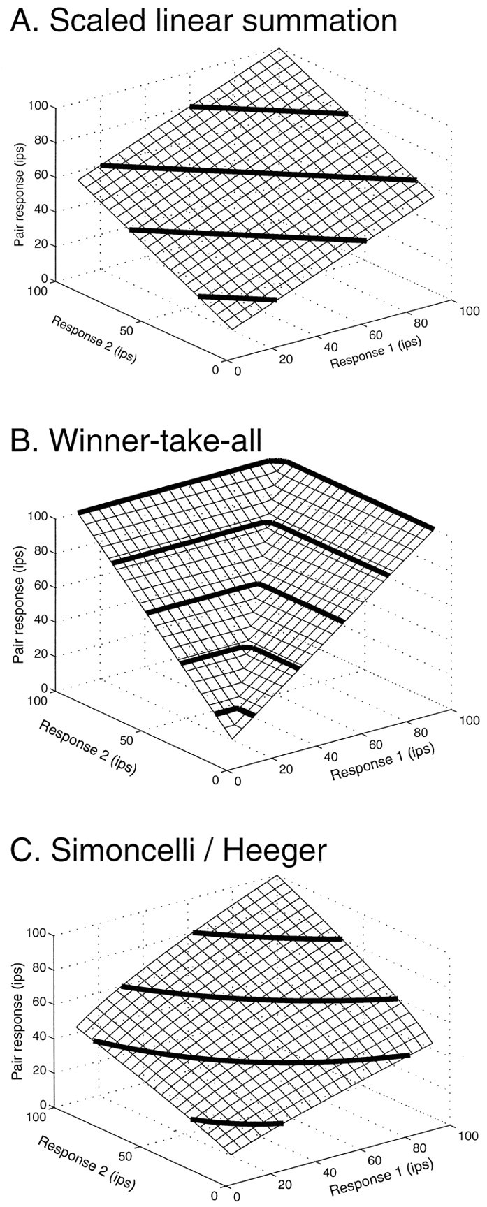
Comparison of predictions of three models for this experiment. A, Linear model: a = 0.5; n = 1. B, Winner-take-all model: a = 1; n = 100.C, Summation followed by squaring: a= 0.0025; n = 0.5. For comparison, the fit values for the two cells portrayed in Figure 6 were Figure6A: a = 0.72;n = 1.36; Figure 6B:a = 0.93; n = 6.68.

The model illustrated in Figure 8C is a reduced version of the model developed by Simoncelli and Heeger (1998), which is also a member of this family of models. In their model, MT cells sum their inputs linearly and then use a “half-squaring” (quadratic) nonlinearity after summation. This corresponds to an exponent of 0.5 in Equation 3. (The square root operation applied to each term in the sum recovers the “underlying linear response,” and the summed quantity is then squared.) The divisive normalization factor in their model depends on total contrast, which is constant in our experiment. Thus the scale constant, a, is equivalent in our model and will be less than unity for divisive normalization.

We have fit various versions of this model to the data resulting from our experiments, and Table 1 summarizes the quality of their account of out data. All models performed acceptably, because all generally agreed with the dominant trend in the data, rising from the left front corner in a portrayal like those in Figure 6, up toward the back right corner. However, some models clearly performed better than others. Both winner-take-all (deep concavity in the surface) and the model of Simoncelli and Heeger (1998) (modest convexity) provided poor accounts of the data. Simple linear averaging fit somewhat better, but allowing the slope to vary noticeably improved the fit, accounting for an additional 4% of response variance on average. This improvement was significant in 61 of 70 cells (nested log-likelihood test, p < 0.05). By comparison, if the exponent is allowed to vary, but the slope is forced to unity, the fits are on average somewhat worse than simple averaging. Unsurprisingly, the best account of the data is provided by the model that allows both scale factor and exponent to vary, and this captures 75% of the observed variance in response, on average. This is an additional 7% of the variance over the scaled linear model on average, and this improvement was significant for 63 of 70 cells.

Table 1.

Model performance comparison

Model	Scale (a)	Exponent (n)	Variance (%)	SD
Winner-take-all	1	100	58	29
Average	0.5	1	64	18
Scaled linear summation	Free	1	68	17
Unscaled power-law summation	1	Free	62	28
Scaled power-law summation	Free	Free	75	18
Simoncelli and Heeger (1998)	Free	0.5	62	16

For each model, we calculated the average percentage of variance accounted for according to the method of Carandini et al. (1997), and the mean value is shown. For this analysis, two cells with limited dynamic range, which were not well fit by any model, were discarded.n = 70.

Figure 9 shows a more detailed comparison among three of these models: scaled linear, Simoncelli and Heeger (1998), and scaled power-law summation. In Figure 9A, we see that the fits for the Simoncelli–Heeger model are systematically worse than the linear model, although both incorporate a free scale factor (“normalization constant”). In Figure 9B, we see that allowing the exponent to vary consistently improves the fits, as one would expect from the performance comparisons described above. Thus, the individual cells in the sample are quite consistent with regard to which summation model best describes these data.

Fig. 9.

Comparison of variance accounted for by three models. Variance accounted for was calculated as 100 * (1 − var(obs − pred)/var(obs)). A, Linear model compared against the model of Simoncelli and Heeger (1998).B, Linear model compared against the generalized power-law summation model. Note that all three models provided fair accounts of the data but also that the generalized model provided the consistently lowest errors.

Finally, we examined the sample distributions for the best-fit parameters to the model that provided the best account of the data: the scaled power-law summation model. The sample distributions of the scale factor and exponent terms (a and n in Equation 3) are shown in Figure 10. This shows that on average, the responses to pairs of stimuli are less than expected from unscaled, linear summation by a substantial amount. In our experiment, this scale factor was almost exactly halfway between averaging (0.5) and summation (1.0). Second, Figure10B shows that the summation is on average modestly nonlinear, characterized by an exponent of 2.72. There is, however, substantial diversity of summation behavior. Cells near the left end of the distribution in Figure 10B are essentially linear, whereas the group that goes off scale to the right can be considered to use a winner-take-all rule. This diversity of summation behavior was not correlated across the sample of 70 cells with any independent measure, including responsiveness, maintained activity, RF size, or location. Furthermore, there was no significant relationship between the scale parameter, a, and the exponent, n (all r values < 0.23).

Fig. 10.

Sample histograms for the two key parameters of the generalized power-law summation model. See Results for details.

Spatial effects

All the preceding analysis was based on the assumption that the summation rule was invariant across space, and the response to two stimuli could be predicted from only the response amplitudes to each component stimulus. We have investigated the spatial dependence of summation in two ways. First, we will describe the average sample summation as a function of the spatial location of each stimulus, which is model-free and descriptive. Then we will explore the residuals to the model fits as a function of stimulus location. The latter analysis investigates whether spatial dependence is also necessary, in addition to the amplitude terms included in our summation model.

For both of these analyses, we expressed the location of each component stimulus in terms of ς, derived from the two-dimensional Gaussian fits to the single-stimulus data. The Gaussian fits (derived from Eq.2) provided two different ς values if the RF was elliptical, and in such cases, a single ς was derived for each stimulus location from its position with respect to the principal axes of the ellipse. Thus, each stimulus location is expressed in terms of its radial location in a standard RF. Figure11A shows the average normalized response (analogous to the portrayal in Fig. 7) as a function of the stimulus locations. On this response surface, the contour lines depict lines of constant average response. One can see that these contours remain parallel to the axes for most of their lengths. In these areas, moving one stimulus has relatively little effect on the response. This is especially true once one or the other stimulus is beyond ∼1 ς in radial position. Thus, moving the second stimulus away from the RF does not allow the response to rise very much. In other words, the scaling influence of a stimulus on MT cell responses is still very much in effect with one or the other stimulus well away from the RF (note the height of the highest contours near each axis).

Fig. 11.

Responses and model residuals as a function of spatial location of the component stimuli. A, Average responses normalized as in Figure 7. B, Residuals from the best-fit generalized power-law summation model, also normalized to the same value, the amplitude of the Gaussian function fit to the single stimulus data.

We have also analyzed the residuals to our best-fitting power-law summation model as a function of stimulus location, and the results of this analysis are shown in Figure 11B. The surface clearly systematically deflects upward along the x- andy-axes, indicating that the nonlinear summation model systematically underestimated the responses when one or the other (but not both) stimuli departed the RF. However, this underestimation was modest in magnitude: only ∼5% at a distance of 2–3 RF radii from the RF center. This is at a location where the first-order response of the cell to the stimulus is effectively zero. Thus, stimuli that are largely ineffective at driving the cell because they lie outside the classical excitatory RF center are still effective at normalizing the responses to stimuli within the RF, and summation and normalization are effectively constant across a region substantially larger than the RF of the cell. The distance over which normalization operates is large: the average RF diameter in our data set was ∼9°. Therefore, it appears that stimuli divisively interact in MT over distances of at least 20°.

Temporal effects

We know that the responses to many different kinds of stimuli adapt rapidly to repeated or continuous presentation, owing to synaptic depression (Abbott et al., 1997) or spike rate adaptation (Connors and Gutnick, 1990). Interaction between such adaptation and the divisive interactions would be of considerable interest, because this would suggest the two processes share biophysical mechanisms. Our rapid, high-contrast stimuli provoked substantial adaptation during the 3 sec trials, which declined during the 2 sec intertrial interval. We may thus relate the time course of neuronal adaptation to the time course of the interaction between stimuli. To do this, we measured the responses of our neurons as a function of order within a trial for both the single and paired stimuli. Figure12 shows the results of this analysis. Figure 12A shows the decline in response during a trial for stimuli presented individually. To derive the averageZ scores, two steps were needed. First, cumulative means and SDs were calculated for each stimulus location in the grid. Then, for each stimulus within a trial, the Z score was calculated by reference to the statistics for that spatial location. TheseZ scores standardize all stimuli so that they can be averaged. One can see that the average response drops substantially across the first three stimuli in a trial (375 msec) and somewhat more slowly for the next several hundred msec. Thus, the expected response is clearly dependent on time.

Fig. 12.

Effects of time on responses to paired stimuli.A, Responses to single-motion impulses, shown as a function of time within a trial. Z scores were calculated relative to the entire distribution of responses to each stimulus location, independent of time, and then averaged for each time position, across stimulus location. Responses clearly decline rapidly in the first 500 msec of each trial (four stimuli). B, Responses to pairs of stimuli, compared against the expected response for that location and time position. Because the stimulus sequence was random, many stimulus location–time position combinations were not represented in any given experiment, but all that were presented contribute to this average. For both Aand B, the error bars denote the SEM across cells.

Knowing that the predicted response should vary within a trial, we can now ask whether the summation behavior also varies. To do this, we again looked at the residuals from the power-law summation model, but now as a function of time within a trial. For each stimulus pair, we first select the single-stimulus presentations for the same point in time to make the model prediction and then calculate the residual from those predictions. In Figure 12B, we show the average residuals to the model fits. We know from Figure 11Athat response falls with time; this asks whether normalization is additionally affected by time. Figure 12B shows that there is a modest effect of time: the residuals are positive for the first 625 msec before declining to near zero values. Although it is possible that this dependence is simply an amplitude–summation nonlinearity not captured by our model, rather than a true effect of time, we think this is unlikely, because in that case the residuals would be expected to fall with the rate change seen in Figure12A. At the very least, one would expect the first stimulus presentation, which has the largest rate, to show the greatest effect, and it does not. Thus, there appears to be a true time dependence of the divisive interactions in MT, which evolves over a few hundred msec, but which is modest in amplitude, because the residuals were never large. Most of the inhibitory interactions are clearly in effect in the first stimulus period (125 msec), so the process appears quite rapid.

DISCUSSION

In this paper we have explored the manner in which brief, localized stimuli interact within the RFs of MT cells. We found that the response to pairs of local motion impulses fell well short of the response expected from summation of the individual component responses. Although responses were well predicted by scaled, linear summation of the inputs, the prediction was markedly improved by using power-law summation. The divisive scaling is not highly dependent on the exact spatial location of the stimuli, but is consistent across a wide region, extending well beyond the classical RF center. We have also studied the interaction as a function of time within a trial, because our stimuli were presented in a rapid sequence, allowing fairly fine sampling of the temporal dimension. The responses dropped rapidly at the onset of the trial, in the first 500 msec, but the interaction between stimuli changed little in this same period. This suggests that divisive normalization is at least partially a separate process from response adaptation.

Technical issues

The single- and double-stimulus pairs were presented in separate blocks lasting at least 10–15 min. If the normalization process were very slow and took seconds or minutes to change states, then both main results of this paper would be called into question. We have considered this issue, and there are two principal arguments against such slow mechanisms. First, the normalization is nearly identical if the single- and double-stimulus conditions are interleaved, as is shown in related work from our laboratory. For the comparable cases as presented in this paper, the median slope relating observed and predicted responses is 0.745, a value nearly identical to the value of 0.745 reported in this paper (H. W. Heuer and K. H. Britten, unpublished observations).

These results, which are beyond the scope of the present paper, also help resolve a potential ambiguity in the present work. Because firing rate is monotonically related to both spatial location in the RF and to the temporal order of stimuli, it is in principle difficult to distinguish amplitude summation effects from spatial or temporal effects. In our more recent experiments (Heuer and Britten, unpublished observations), contrast was varied as well as spatial location, allowing the disambiguation of firing rate and location. In preliminary analysis of these results, the spatial pattern of residuals appears very similar to that seen in Figure 11. Therefore, we are confident in our estimates of the spatial extent of the divisive normalization.

Relationship to previous work

Several studies have addressed the responses of MT cells to multiple moving stimuli in their RFs. Studies using plaid grating stimuli have tended to focus on directional tuning, rather than amplitude of the responses (Movshon et al., 1985; Rodman and Albright, 1989; Stoner and Albright, 1992). Because we do not vary direction, we cannot compare our results with these. Several studies have, however, quantitatively analyzed the amplitude of responses to multiple stimuli, but none have yet addressed the spatial location of the stimuli.Snowden et al. (1991) measured responses to transparently presented dot fields, whereas Recanzone et al. (1997) and Ferrera and Lisberger (1997) have used pairs of dots traversing the RFs of MT cells. The consensus finding from these studies is that MT cells average multiple inputs using some form of divisive operation. The present work extends these observations by exploring their dependence on spatial location, and we find that the normalization extends well beyond the classical RF center. In the present data, we find somewhat less normalization than previous studies in which the effects of space were not explored. The divisive scale factor we found was 0.75, whereas Recanzone et al. (1997) reported that averaging (0.5) slightly overestimatesthe response. Snowden et al. (1991) used a slightly different metric and reported an average value indicating near perfect averaging. On the other hand, Ferrera and Lisberger (1997) explored the influence of a second moving stimulus near but outside the RF of MT cells. Although it is difficult to know how far their “distractor” stimuli were from the RF, from what they present, they consistently observe no effect of the second stimulus on the response of the MT cells to a preferred stimulus (a = 1.0 in our notation). Although it is possible that differences in the stimuli or the fact that they recorded from cells with more central RFs might explain the difference in results, a more parsimonious explanation is that their distractor stimuli were farther from the RF, and that the divisive inhibition had declined by this distance.

The comparison with the results of Ferrera and Lisberger (1997) also helps with respect to any potential involvement of antagonistic surround mechanisms (Allman et al., 1985; Born and Tootell, 1992;Raiguel et al., 1995). The smallest stimuli that have been used to measure surround effects are dot fields subtending a substantial fraction of the RF width (Raiguel et al., 1995). The much smaller stimuli of Ferrera and Lisberger (1997) probably do not trigger surround modulation. Although we cannot rule out activation of surround mechanisms in the present experiments, we suspect that our small, transient stimuli more resemble the moving dots of the experiments of Ferrera and Lisberger and probably do not much influence the surround. Detailed examination of the relationship between divisive interactions in the center and surround mechanisms (which are often considered subtractive) is clearly an important direction for future work.

One feature of the present work, not previously reported, is the nonlinear summation captured by the value of the exponent in our power-law summation model. Because space and response strength covary in our measurements, this term must be viewed with some caution. We have argued in Results against such an interpretation, but it remains open. No other work on MT has explicitly considered nonlinear summation, but in work on simple cells in V1 by Carandini et al. (1997), a related nonlinearity helps describe the summation of pairs of superimposed grating stimuli varying in contrast. Interestingly, although their biophysically motivated model differs from ours in many ways, the average value of their exponent is very close to ours (2.34–2.61 vs 2.72). It is also very interesting that in the “selection model” of Nowlan and Sejnowski (1995), normalized, nonlinear summation is used.

Mechanism

The measurements in the present work allow further constraint on possible mechanisms of divisive normalization. Specifically, these interactions can be seen to occur across wide regions of space. In many of our experiments, stimuli were 10–20° apart. Normalization was still effective at these distances, probably beyond the extent of lateral connections in V1. Although these observations do not exclude normalization in V1 as one component, they suggest that an additional step at MT is also necessary. Because normalization is effective even for stimuli well outside the RF, which evoke little response by themselves, it also seems necessary to invoke lateral connections from neurons that are activated by these stimuli. Otherwise, if some homosynaptic or recurrent gain control were operating, its effectiveness would be expected to fall with the main excitatory effect of the stimulus. This is clearly not supported by the data.

Two types of mechanism appear to satisfy the constraints imposed by the present data. One is lateral inhibitory networks within MT. These would presumably connect in a mutually inhibitory manner cells with largely, partially, or barely overlapping RFs. Decline in the density of such connections would then explain the declining effectiveness of normalization at distances of 2–3 RF radii. Another possibility involves feedback from higher areas, such as MST. Recent observations suggest that feedback from MT is important in center–surround interactions in V1 (Hupe et al., 1998); an analogous operation might allow MST feedback to modulate divisive interactions in MT. Two observations argue against this possibility, in our view. First, the rapid kinetics of the divisive interactions we observe seem to render it less likely: the inhibition appears to be in effect in the first 125 msec. Second, the connections between MT and MST are topographically imprecise (Maunsell and Van Essen, 1983a; Boussaoud et al., 1990). Thus, feedback-dependent inhibition might be expected to be even less dependent on spatial location than what we observe in the present study. However, either mechanism remains possible at present.

We have termed the divisive interactions normalization, consistent with one recent model of MT cell responses. The main function of this mechanism is to keep the representation of direction (or anything else that is represented) approximately invariant in the face of changing stimulus contrast. This is because animals rarely care about the contrast of an object; it is more important to determine object attributes such as direction of motion. To fully test the relationship between the phenomenon we have described and contrast normalization, we will need to measure the contrast dependence of these divisive interactions. Work addressing this question is presently under way in our laboratory.

REFERENCES

- 1.Abbott LF, Varela JA, Sen K, Nelson SB. Synaptic depression and cortical gain control [see comments]. Science. 1997;275:220–224. doi: 10.1126/science.275.5297.221. [DOI] [PubMed] [Google Scholar]
- 2.Allman JM, Meizin F, McGuinness E. Direction and velocity-specific responses from beyond the classical receptive field in the middle temporal visual area (MT). Perception. 1985;14:105–126. doi: 10.1068/p140105. [DOI] [PubMed] [Google Scholar]
- 3.Born RT, Tootell RB. Segregation of global and local motion processing in primate middle temporal visual area. Nature. 1992;357:497–499. doi: 10.1038/357497a0. [DOI] [PubMed] [Google Scholar]
- 4.Boussaoud D, Ungerleider LG, Desimone R. Pathways for motion analysis: cortical connections of the medial superior temporal and fundus of the superior temporal visual areas in the macaque. J Comp Neurol. 1990;296:462–495. doi: 10.1002/cne.902960311. [DOI] [PubMed] [Google Scholar]
- 5.Britten KH. Spatial interactions within monkey middle temporal (MT) receptive fields. Soc Neurosci Abstr. 1995;21:663. [Google Scholar]
- 6.Britten KH, Newsome WT. Responses of MT neurons to discontinuous motion stimuli. Invest Opthalmol Vis Sci [Suppl] 1990;31:238. [Google Scholar]
- 7.Carandini M, Heeger DJ, Movshon JA. Linearity and normalization in simple cells of the macaque primary visual cortex. J Neurosci. 1997;17:8621–8644. doi: 10.1523/JNEUROSCI.17-21-08621.1997. [DOI] [PMC free article] [PubMed] [Google Scholar]
- 8.Connors BW, Gutnick MJ. Intrinsic firing patterns of diverse neocortical neurons. Trends Neurosci. 1990;13:99–104. doi: 10.1016/0166-2236(90)90185-d. [DOI] [PubMed] [Google Scholar]
- 9.Crist CF, Yamasaki DSG, Komatsu H, Wurtz RH. A grid system and a microsyringe for single cell recording. J Neurosci Methods. 1988;26:117–122. doi: 10.1016/0165-0270(88)90160-4. [DOI] [PubMed] [Google Scholar]
- 10.Ferrera VP, Lisberger SG. Neuronal responses in visual areas MT and MST during smooth pursuit target selection. J Neurophysiol. 1997;78:1433–1446. doi: 10.1152/jn.1997.78.3.1433. [DOI] [PubMed] [Google Scholar]
- 11.Gallyas F. Silver staining of myelin by means of physical development. Neurol Res. 1979;1:203–209. doi: 10.1080/01616412.1979.11739553. [DOI] [PubMed] [Google Scholar]
- 12.Hays AV, Richmond BJ, Optican LM. A UNIX-based multiple process system for real-time data acquisition and control. WESCON Conf Proc. 1982;2:1–10. [Google Scholar]
- 13.Hupe JM, James AC, Payne BR, Lomber SG, Girard P, Bullier J. Cortical feedback improves discrimination between figure and background in V1, V2 and V3 neurons. Nature. 1998;394:784–787. doi: 10.1038/29537. [DOI] [PubMed] [Google Scholar]
- 14.Judge SJ, Richmond BJ, Chu FC. Implantation of magnetic search coils for measurement of eye position: an improved method. Vision Res. 1980;20:535–538. doi: 10.1016/0042-6989(80)90128-5. [DOI] [PubMed] [Google Scholar]
- 15.Maunsell JHR, Van Essen DC. The connections of the middle temporal visual area (MT) and their relationship to a cortical hierarchy in the macaque monkey. J Neurosci. 1983a;3:2563–2586. doi: 10.1523/JNEUROSCI.03-12-02563.1983. [DOI] [PMC free article] [PubMed] [Google Scholar]
- 16.Maunsell JHR, Van Essen DC. Functional properties of neurons in the middle temporal visual area (MT) of the macaque monkey: I. Selectivity for stimulus direction, speed and orientation. J Neurophysiol. 1983b;49:1127–1147. doi: 10.1152/jn.1983.49.5.1127. [DOI] [PubMed] [Google Scholar]
- 17.Movshon JA, Newsome WT. Visual response properties of striate cortical neurons projecting to area MT in macaque monkeys. J Neurosci. 1996;16:7733–7741. doi: 10.1523/JNEUROSCI.16-23-07733.1996. [DOI] [PMC free article] [PubMed] [Google Scholar]
- 18.Movshon JA, Adelson EH, Gizzi MS, Newsome WT. The analysis of moving visual patterns. In: Chagas C, Gattass R, Gross C, editors. Study group on pattern recognition mechanisms. Pontifica Academia Scientiarum; Vatican City: 1985. pp. 117–151. [Google Scholar]
- 19.Nowlan SJ, Sejnowski TJ. A selection model for motion processing in area MT of primates. J Neurosci. 1995;15:1195–214. doi: 10.1523/JNEUROSCI.15-02-01195.1995. [DOI] [PMC free article] [PubMed] [Google Scholar]
- 20.Press WH, Flannery BP, Teukolsky SA, Vetterling WT. Numerical recipes in C. Cambridge UP; Cambridge, UK: 1988. [Google Scholar]
- 21.Raiguel S, Van Hulle MM, Xiao DK, Marcar VL, Orban GA. Shape and spatial distribution of receptive fields and antagonistic motion surrounds in the middle temporal area (V5) of the macaque. Eur J Neurosci. 1995;7:2064–2082. doi: 10.1111/j.1460-9568.1995.tb00629.x. [DOI] [PubMed] [Google Scholar]
- 22.Raiguel S, Van Hulle MM, Xiao DK, Marcar VL, Lagae L, Orban GA. Size and shape of receptive fields in the medial superior temporal area (MST) of the macaque. NeuroReport. 1997;8:2803–2808. doi: 10.1097/00001756-199708180-00030. [DOI] [PubMed] [Google Scholar]
- 23.Recanzone GH, Wurtz RH, Schwarz U. Responses of MT and MST neurons to one and two moving objects in the receptive field. J Neurophysiol. 1997;78:2904–2915. doi: 10.1152/jn.1997.78.6.2904. [DOI] [PubMed] [Google Scholar]
- 24.Rodman HR, Albright TD. Single-unit analysis of pattern-motion selective properties in the middle temporal visual area (MT). Exp Brain Res. 1989;75:53–64. doi: 10.1007/BF00248530. [DOI] [PubMed] [Google Scholar]
- 25.Simoncelli EP, Heeger DJ. A model of neuronal responses in visual area MT. Vision Res. 1998;38:743–761. doi: 10.1016/s0042-6989(97)00183-1. [DOI] [PubMed] [Google Scholar]
- 26.Snowden RJ, Treue S, Erickson RG, Andersen RA. The response of area MT and V1 neurons to transparent motion. J Neurosci. 1991;11:2768–2785. doi: 10.1523/JNEUROSCI.11-09-02768.1991. [DOI] [PMC free article] [PubMed] [Google Scholar]
- 27.Sokal RR, Rohlf FJ. Biometry. Freeman; San Francisco: 1969. [Google Scholar]
- 28.Stoner GR, Albright TD. Neural correlates of perceptual motion coherence. Nature. 1992;358:412–414. doi: 10.1038/358412a0. [DOI] [PubMed] [Google Scholar]
- 29.Tanaka K, Hikosaka H, Saito H, Yukie Y, Fukada Y, Iwai E. Analysis of local and wide-field movements in the superior temporal visual areas of the macaque monkey. J Neurosci. 1986;6:134–144. doi: 10.1523/JNEUROSCI.06-01-00134.1986. [DOI] [PMC free article] [PubMed] [Google Scholar]
- 30.Watson AB, Turano K. The optimal motion stimulus. Vision Res. 1995;35:325–336. doi: 10.1016/0042-6989(94)00182-l. [DOI] [PubMed] [Google Scholar]