Electromyographic Correlates of Learning an Internal Model of Reaching Movements

Abstract

Theoretical and psychophysical studies have suggested that humans learn to make reaching movements in novel dynamic environments by building specific internal models (IMs). Here we have found electromyographic correlates of internal model formation. We recorded EMG from four muscles as subjects learned to move a manipulandum that created systematic forces (a “force field”). We also simulated a biomechanical controller, which generated movements based on an adaptive IM of the inverse dynamics of the human arm and the manipulandum. The simulation defined two metrics of muscle activation. The first metric measured the component of the EMG of each muscle that counteracted the force field. We found that early in training, the field-appropriate EMG was driven by an error feedback signal. As subjects practiced, the peak of the field-appropriate EMG shifted temporally to earlier in the movement, becoming a feedforward command. The gradual temporal shift suggests that the CNS may use the delayed error–feedback response, which was likely to have been generated through spinal reflex circuits, as a template to learn a predictive feedforward response. The second metric quantified formation of the IM through changes in the directional bias of each muscle’s spatial EMG function, i.e., EMG as a function of movement direction. As subjects practiced, co-activation decreased, and the directional bias of each muscle’s EMG function gradually rotated by an amount that was specific to the field being learned. This demonstrates that formation of an IM can be represented through rotations in the spatial tuning of muscle EMG functions. Combined with other recent work linking spatial tunings of EMG and motor cortical cells, these results suggest that rotations in motor cortical tuning functions could underlie representation of internal models in the CNS.

People learn to move novel objects along desired trajectories, in any direction, by simply practicing the task a few times. This adaptation is remarkable because of the computational complexity inherent to learning dynamics (Atkeson, 1989). Adaptation of a neural internal model (IM), transforming desired trajectories of the hand into appropriate muscle activations, likely underlies this ability (Jordan, 1995; Wolpert et al., 1995). Aftereffects, errors that people make when learned dynamics are unexpectedly changed, suggest that IMs are built gradually with practice (Shadmehr and Mussa-Ivaldi, 1994), that learning one IM can interfere with the learning of a second IM (Brashers-Krug et al., 1996), and that the interference fades over the course of hours (Shadmehr and Brashers-Krug, 1997). The evidence for the formation of IMs, however, comes mainly from psychophysics. A measure of neural output, such as electromyography (EMG), could provide insight into the neural basis of the formation of IMs.

Previous work has reported EMG changes during learning of single-joint movements with different loads (Corcos et al., 1993; Gottlieb, 1994). When subjects make elbow movements against an unexpected load, EMG patterns up until 200 msec into the movement remain unchanged compared with unperturbed trials (Gottlieb, 1996). This delayed response to the perturbation reflects the latency of short- and long-loop reflexes that use proprioceptive information to produce an error–feedback action (Marsden et al., 1978). Once subjects practice with the novel load, EMG differs from unperturbed trials from the beginning of movement (Gottlieb, 1994). This change in the movement-initiating EMG reflects the adaptation of descending control commands. In computational studies, the changes in descending commands are attributable to adaptation of an IM (Wada and Kawato, 1993; Miall and Wolpert, 1996;Barto et al., 1998; Bhushan and Shadmehr, 1999). An elegant idea is that adaptation may be driven by error–feedback motor responses generated by reflex circuits (Kawato et al., 1987; Stroeve, 1997). In other words, the delayed, reflex-based error feedback might serve as a “blueprint” for how the CNS needs to change descending commands. To test this idea, the computational concept of an IM for multijoint movements needs to be described in a way that its formation could be quantitatively tested by changes in EMG. Here we asked whether changes in EMG correlate with the formation of an IM, and whether the error–feedback response drives this learning.

We measured EMG as subjects learned to reach while grasping a manipulandum, which created novel forces. We used a biomechanical model to transform EMG into a composite trace, corresponding to activation that specifically compensated for the imposed field. We found that with training, activation of the appropriate musculature gradually shifted from a delayed error–feedback response to a predictive feedforward response. To quantify how these changes corresponded to the formation of an IM, we analyzed the directional tuning functions of movement-initiating EMG. These spatial functions relate EMG to movement direction in hand-centered coordinates (Flanders and Soechting, 1990; Sergio and Kalaska, 1998). Previous reports have demonstrated that reaching movements or isometric force production generate EMGs with broadly tuned directional biases (Flanders and Soechting, 1990; Flanders, 1991; Karst and Hasan, 1991). Our modeling revealed that learning of an IM should result in specific rotations of muscles’ tuning curves. We found that with practice, the directional patterns of activation gradually rotated; the final magnitude of the rotations corresponded well with the predicted change. Temporal features and angular orientation are invariant to the overall magnitude of the EMG; therefore, across subjects and across recording sessions, despite removal and reapplication of surface electrodes, our metrics robustly quantified the formation of internal models.

Portions of this work have been presented previously in abstract form (Thoroughman and Shadmehr, 1998).

MATERIALS AND METHODS

Experimental apparatus. Twenty-four right-handed subjects (12 women and 12 men), students in the Johns Hopkins School of Medicine, provided written consent to participate in this study. With their right hand, subjects grasped the end effector (handle) of a 2 df manipulandum mounted in the horizontal plane (Shadmehr and Brashers-Krug, 1997). Subjects sat in front of the manipulandum, with the right arm supported by a sling. Sensors on the manipulandum accurately measured joint position and velocity (details provided byShadmehr and Brashers-Krug, 1997). Two motors, mounted on the base of the manipulandum, could independently produce torque on the proximal and distal joints of the robotic arm. A computer monitor mounted above the manipulandum displayed a cursor representing hand position and boxes representing targets. Using pediatric cardiac electrodes, EMG was recorded from four muscles: biceps, triceps lateralis/longus, anterior deltoid, and posterior deltoid. Before the application of the electrodes, the skin was cleaned and abraded using a preparation gel (NuPrep; Weaver, Aurora, CO). EMG signals were amplified by Grass (Quincy, MA) AC amplifiers (model 8A5) with 60 Hz notch filters. The amplified signal was bandpass-filtered (17–530 Hz), processed through a root-mean-square circuit with a 25 msec integration window (De Luca, 1997), and digitized. Hand position, hand velocity, and processed EMG were recorded at 100 Hz. The processed and digitized EMG formed the signals analyzed below.

Experimental protocol. Subjects made 10 cm point-to-point movements toward 8 mm square targets represented by boxes on the computer monitor. Subjects made movements in four directions (0, 45, 90, and 135°) away from the center of the work space and four directions (180, 225, 270, and 315°) back to the center; the order of the outward directions was determined pseudorandomly. If subjects completed the movement in 500 ± 50 msec, the box “exploded,” and the computer generated a pleasing sound. If the cursor reached the box too slowly (in ≥550 msec), the target filled in blue; if the cursor reached the box too quickly (in ≤450 msec), the target filled in red. The only instruction provided was to explode as many targets as possible. We provided no instructions regarding straightness of movements or smoothness of trajectories.

Subjects made reaching movements in two or three different dynamic environments. One, termed the “null field,” is the condition in which the torque motors do not create any forces; in the null field the subjects encounter only the inertial dynamics of the manipulandum. In the second and third environments, B₁ andB₂, torque motors produce an additional force as described by the equation:

$$\vec{F}=\mathbf{B}\vec{\dot{x}},$$ Equation 1

where F⃗ is the force produced at the end effector by the robot’s motors, $\vec{\dot{x}}$ is the instantaneous velocity vector of the hand, and B is a viscosity matrix. In the first environment, the null field,B₀ equals [0 0; 0 0] N · sec · m⁻¹. In the second environment,B₁ equals [0 13; −13 0] N · sec · m⁻¹; in the third,B₂ = −B₁. These “force fields” exert a force proportional in strength to the instantaneous speed of the hand, in the direction perpendicular to the instantaneous velocity vector.

Subjects’ training was divided into sets of 192 movements. Each set was followed by a 3 min rest period. On a first day of training, all 24 subjects completed three sets of movements in the null field. On a second day, all subjects completed one set in the null field and then three sets in the force field B₁. Here we report data only from the second day.

After completion of the training in B₁, three groups of eight subjects each completed two sets of movements. One group completed these two sets in the null field after the standard 3 min rest. A second group trained in B₂ 3 min after B₁, and a third group trained inB₂ 6 hr after B₁. During the 6 hr period, EMG electrodes were removed, and subjects left the laboratory. After their return, electrodes were reapplied on approximately the same arm positions as the earlier session, as marked by the earlier abrasion of the skin.

Displacement analysis. To facilitate averaging across movements, all movement data were temporally aligned on the basis of the movement onset, which was defined as when the tangential speed first crossed a threshold (0.03 m/sec). Perpendicular velocity was defined as the component of the velocity vector that pointed perpendicular to the line connecting the initial hand position and target position. Perpendicular displacement was computed by summing perpendicular velocity over the first 250 msec of the movement. In each direction we subtracted away the average perpendicular displacement generated in the null field (first set, day 2).

EMG normalization. Each subject’s (bandpassed, RMS’d) EMG traces were normalized based on movement-initiating EMG recorded during the initial null field set. For each muscle m and in each direction of movement, we calculated a scalar activation a_m by averaging the EMG trace A_m(t) over time interval between 50 msec before and 100 msec after the onset of movement (capital letters refer to full time series; small letters refer to scalar measures) and then averaging over all movements made in that direction during the initial null field set. We constructed an 8 × 1 vectora⃗_m for each muscle, each element representing a single direction. We then adjusted the scale of each muscle’s EMG trace in each movement, producing the normalized trace Aⁿ, using the equation:

$$A_{k,m}^n(t)=50\ast \frac{A_{k,m}(t)-min({\vec{a}}_m)}{max({\vec{a}}_m)-min({\vec{a}}_m)}+25,$$ Equation 2

where k is an index of movement number, and m is an index of muscle. Within each subject, therefore, the EMG values recorded during all movements (in the null field and in force fields) were normalized using the same linear transformation. This transformation facilitated comparisons of activation across subjects but preserved the training-induced changes of every subject’s EMG.

Polar analysis. We used a form of data analysis termed polar analysis to evaluate changes in EMG. We began the analysis by computing the movement-initiating activation for each subject, binned within each direction across eight movements. We then multiplied each scalar by the unit vector pointing in the direction of movement, so that these vectors, when plotted together, display a_m as radii pointing in the direction of movement corresponding to that activity. These polar plots summarized the function mapping target direction into initial EMG activity.

To determine the directional bias of each activation function, in each movement bin we added the eight a_m vectors together to form one resultant vector. This resultant vector had the same direction and is proportional in magnitude to the mean of the eight vectors (if a unit mass would have been placed on the end point of each vector, the mean of the vectors would have been the center of mass of the collection of points). By calculating the orientation of this resultant vector, we detected changes in the angular dependence of a_m as subjects learned dynamic environments.

Computational modeling: structure of the model. The purpose of the computational modeling was to predict the change in the pattern of joint torques that should result if an adaptive control system learned to completely compensate for the dynamics of the force field. To calculate the changes in joint torques attributable to adaptation, we simulated the dynamics of the four-link system of Figure1 through the following coupled differential equations:

$${\mathbf{I}}_r(\vec{p})\ddot{\vec{p}}+{\mathbf{G}}_r(\vec{p},\dot{\vec{p}})\dot{\vec{p}}=\mathbf{M}(\dot{\vec{p}})+{\mathbf{J}}_r^T\vec{F};$$ Equation 3

$${\mathbf{I}}_s(\vec{q})\ddot{\vec{q}}+{\mathbf{G}}_s(\vec{q},\dot{\vec{q}})\dot{\vec{q}}=\vec{C}(\vec{q},\dot{\vec{q}},\vec{q}*(t))-{\mathbf{J}}_s^T\vec{F},$$ Equation 4

where I and G were inertial and coriolis/centripetal matrix functions, M was the torque field produced by the robot’s motors, i.e., the environment,F⃗ was the force vector measured at the handle of the robot, C⃗ was the adaptive controller implemented by the motor system of the subject, q⃗*(t) was the reference trajectory planned by the motor control system of the subject, J_r was the Jacobian matrix describing the differential transformation of coordinates from end point to joints, q⃗ and p⃗ were column vectors representing joint positions of the subjects and the robot (Figure 1), and the subscripts s and r denoted subject or robot matrices of parameters.

Fig. 1.

Experimental apparatus. Subjects make reaching movements while grasping a 2 df manipulandum (robotic arm). The manipulandum could be programmed to produce a force field.

The robot’s passive mechanical dynamics,I_r and G_r, as well as a typical subject’s passive dynamics of the arm,I_s and G_s, were previously estimated (Shadmehr and Brashers-Krug, 1997). A key design question is with respect to the function C. Simulations have previously suggested that a reasonable lumped model of the subject’s biomechanical controller in the case of these targeted movements is as follows (Shadmehr and Brashers-Krug, 1997):

$$\vec{C}={\widehat{\mathbf{I}}}_s(\vec{q}*)\vec{q}*+{\mathbf{G}}_s(\vec{q}*,\dot{\vec{q}}*)\dot{\vec{q}}*-\widehat{\mathbf{M}}(\dot{\vec{q}}*)-\mathbf{K}(\vec{q}-\vec{q}*)-\mathbf{V}(\dot{\vec{q}}-\dot{\vec{q}}*).$$ Equation 5

K was a linear estimate of the subject’s joint stiffness and was set to a constant K = [15, 6; 6, 16] N · m⁻¹ · rad⁻¹ (Mussa-Ivaldi et al., 1985). V was a linear estimate of joint viscosity and was set at V = [2.25, 0.9; 0.9, 2.4] N · m⁻¹ · sec⁻¹ · rad⁻¹. This controller is dependent on a model of the subject’s passive dynamics, represented by Î_s andĜ_s, and model of the force field environment, M̂(q˙*). We assumed the desired trajectory, q⃗*(t), was a minimum jerk motion of the hand to the target (Flash and Hogan, 1985) with a period of 0.5 sec. Our previous simulations have suggested that such a controller produced trajectories in the above differential equations that reasonably agreed with performance of our subjects in the field (Shadmehr and Brashers-Krug, 1997).

We simulated Equations 3 and 4 for a configuration of the arm in which the hand made the first movement starting from x = −0.1 and y = 0.45 m, based on the coordinate system shown in Figure 1. This is the work space for which the EMG data in the current paper were acquired. The force field produced by the robot was always of the form F⃗ =B $\dot{\vec{x}}$. This field can be written in joint coordinates of the robot or the subject, i.e., the M variable in Equation 3, using simple kinematic transformations (Shadmehr and Mussa-Ivaldi, 1994). We considered two conditions. In the first condition, the field produced by the robot wasB = B₀, i.e., the null field. In the second condition, we had B =B₁. We performed a numerical simulation of Equations 3 and 4 for each condition under the assumption that the controller had a perfect model of the field. Movements were simulated to the same eight directions as in our psychophysical studies.

The torques produced by the controller of Equation 3 on the shoulder and elbow joints were τ_s(t, θ) and τ_e(t, θ), where t is time into the movement, and θ is the target direction. The calculated elbow and shoulder torques were parceled into muscle force by solving the set of equations,

$$\vec{\tau }={\mathbf{J}}_m^T\vec{F}$$ Equation 6

$$F_b{F}_t=k_{\text{bt}}$$

$$F_a{F}_p=k_{\text{ap}},$$

where F⃗ ≡ [F_b, F_t, F_a, F_p]^T is a vector of muscle forces,J_m^T is the transpose of the differential transformation from muscle lengths to joint angles, i.e., dλ/dθ, the Jacobian representing muscle moment arms, and k_bt and k_ap are constants of reciprocal activation. The reciprocal activation constants were derived through analysis of the actual null field EMG data. From the recorded EMG data, a_m was calculated for each muscle for each direction (this represented the average EMG from t = −50 to t = 100 msec into the movement). Next, a resultant vector was calculated for each muscle. The ratio of the length of the resultant vector to the mean of the a_m function for each muscle was calculated. This represented the strength of the directional bias of each muscle’s EMG. We observed that selection of reciprocal activation constants k_bt and k_ap determined the strength of the directional bias of muscle forces in the model (also calculated over t = −50 to t = 100 msec). We adjusted the activation constants in the model so that it produced muscle forces that matched the strength of the directional biases measured in the a_m data. We arrived at k_bt = 1 × 10³ N² and k_ap = 3 × 10³N².

There is no general consensus regarding the magnitude of muscle moment arms (i.e., matrix J_m in Eq. 6) for the human arm in the horizontal plane. Here we considered six different models (Table 1). Four of the matrices (models A–D) were derived presuming different levels of effective biarticulation of biceps and triceps: model A presumed no biarticulation, and models B–D presumed that the moment arms of biceps and triceps across the shoulder were one-half, the same, and twice the moment arms of the anterior and posterior deltoids, respectively. The fifth model (E) was derived from cadaver data (Wood et al., 1989) recorded with the shoulder adducted and forearm horizontal and extending forward, and the sixth model (F) was model E transformed through a rigid body rotation to the horizontal plane of the shoulders.

Table 1.

Computational representation of an internal model in terms of expected changes in the angular orientation of the EMG, as represented by a spatial function in hand centered coordinates, for each muscle

Model	Moment arm matrices (cm) JmT = (dλ/dθ)T	Expected rotation in the muscle’s EMG function when fieldB1 is learned (°)
		Biceps	Triceps	Ant del	Post del
A	$\left[\begin{array}{c} 4\\ \hfill 0\end{array}\begin{array}{c}­4\\ \hfill 0\end{array}\begin{array}{c} 0\\ \hfill 4\end{array}\begin{array}{c} 0\\ \hfill ­4\end{array}\right]$	−26.6	−26.5	−14.1	−13.6
B	$\left[\begin{array}{c} 4\\ \hfill 0\end{array}\begin{array}{c}­4\\ \hfill 0\end{array}\begin{array}{c} 2\\ \hfill 4\end{array}\begin{array}{c}­2\\ \hfill ­4\end{array}\right]$	−26.6	−26.5	−13.2	−13.0
C	$\left[\begin{array}{c} 4\\ \hfill 0\end{array}\begin{array}{c}­4\\ \hfill 0\end{array}\begin{array}{c} 4\\ \hfill 4\end{array}\begin{array}{c}­4\\ \hfill ­4\end{array}\right]$	−26.6	−26.6	−13.7	−13.6
D	$\left[\begin{array}{c} 4\\ \hfill 0\end{array}\begin{array}{c}­4\\ \hfill 0\end{array}\begin{array}{c} 4\\ \hfill 2\end{array}\begin{array}{c}­4\\ \hfill ­2\end{array}\right]$	−26.6	−26.6	−19.7	−20.2
E	$\left[\begin{array}{c} 4.58\\ \hfill 0\end{array}\begin{array}{c}­0.70\\ \hfill 0\end{array}\begin{array}{c} 2.37\\ \hfill 4.67\end{array}\begin{array}{c}­2.74\\ \hfill ­1.48\end{array}\right]$	−26.6	−26.5	−13.1	−16.6
F	$\left[\begin{array}{c} 3.16\\ \hfill 0\end{array}\begin{array}{c}­6.07\\ \hfill 0\end{array}\begin{array}{c} 2.20\\ \hfill 4.84\end{array}\begin{array}{c}­3.43\\ \hfill ­2.21\end{array}\right]$	−26.6	−26.5	−12.7	−15.2

Learning of an internal model is predicted to result in a specific rotation in each muscle EMG function. The magnitude of the predicted rotation depends on the muscle moment arms. Because of a lack of consensus regarding the magnitude of each muscle’s moment arm, we have considered six different models for J_m. In each case, λ is a vector of muscle lengths [biceps, triceps, anterior deltoid (Ant del), and posterior deltoid (Post del)], and θ is a vector of joint angles (shoulder and elbow). The consequence of learning an internal model of field B₁ should be a rotation in the resultant vector of each muscle’s EMG functions from that observed in the null field.

Computational modeling: predicting rotation of directional bias.For each moment arm model, the simulation produced a time series of muscle forces appropriate to make movements in the null field. In each direction of movement i, we averaged over the first 150 msec of predicted force production (corresponding to the interval 50 msec before through 100 msec after movement initiation) to determine for each muscle a scalar variable f_m(i). We performed polar analysis (see above) on these scalars to determine a resultant vector to summarize, in null field movements, the angular dependence of f_m on movement direction. We then performed the same analysis on the forces appropriate to move in the force field B₁. From these two polar analyses we determined, for each muscle, the difference between the orientations of f_m resultant vectors in the null field and in force field B₁.

The results for each model are shown in Table 1. We found that changing moment arm matrices tended to change the orientation of preferred directions in both null field and B₁ but did not tend to change the angle between them. All models predicted approximately the same levels of rotation in the tuning functions of biceps and triceps. For the anterior and posterior deltoids, predicted rotations were very similar for all models except that of model D. The results in Table 1 show how much rotation of the spatial activation function, as represented in hand-centered coordinates, should occur as a subject learns an internal model for fieldB₁.

Computational modeling: predicting time series of appropriate activations. Studies that have recorded EMG during single-joint movements have reported increases or decreases in the activation of individual muscles during learning. This analysis is appropriate for tasks with a single degree of freedom, but here we needed to consider movements with 2 df, actuated by multiple muscles, moving in several directions. To facilitate analysis of EMG across directions of movement, we derived an inverse muscle model, whose parameters were determined by subjects’ EMG in the null field. The model was validated by predicting EMG patterns in the force field. These predictions were then used to remap EMG into composite traces based on their functional relevance.

To determine the muscle activations appropriate for our task, we first used Equations 3-6 and muscle model C to calculate the time series of muscle forces necessary to make a minimum jerk reaching movement, F_i,m,n(t), where i indicates movement direction, m muscle, and n force field (n = 0 signifies the null field, n = 1 the force field B₁). Next, we transformed the modeled muscle force F_i,m,n(t) into appropriate muscle activations. To estimate the relationship between predicted muscle force and recorded EMG [A_i,m,n(t)], we found a piecewise linear fit between the force predictions in the null field and the recorded EMG from our subjects, using the following analyses. In the null field, for each muscle m and in each direction, we calculated the average predicted force and recorded EMG during the agonist period, from 50 msec before through 100 msec after the onset of the movement (f_m^ag and a_m^ag), and during the antagonist period, from 200 msec through 300 msec into the movement (f_m^ant and a_m^ant). We then fit the null field forces across all eight directions to the recorded null field EMG using the equations:

$${\vec{a}}_m^{\text{ag}}=p_m^1 {\vec{f}}_m^{\text{ag}}+p_m^2$$ Equation 7

$${\vec{a}}_m^{\text{ant}}-{\vec{a}}_m^{\text{ag}}=p_m^3({\vec{f}}_m^{\text{ant}}-{\vec{f}}_m^{\text{ag}})+p_m^4,$$

where a⃗ and f⃗ are 8 × 1 vectors reflecting recorded EMG and predicted force in all eight directions, and p are parameters of the fit.

We calculated the parameters to find the least-squared fit of the null field data and found that the fit was significant for all four muscles, during both the agonist and antagonist bursts (for all eight fits, r > 0.88; p < 1 × 10⁻³; the top two plots in Figure2 show the fits for anterior deltoid in the null field). To validate the fits, we used the same parameters to transform f_i,m,1, the predicted force for field B₁, into predicted EMG. The transformed forces fit the mean EMG recorded from the subjects rather well [for one of the fits (triceps during the antagonist burst), r = 0.73; p < 0.04; for all other fits, r > 0.80; p < 0.015; the bottom two plots in Figure 2 show, for anterior deltoid, the relationship between transformed force and EMG in the fieldB₁]. The parameters used for the fits are given in Table 2. This rather simple muscle model, therefore, was validated on data not used to fit the parameters.

Fig. 2.

Data used for building a simple force activation model for the anterior deltoid and data used for testing the validity of the model. We fitted the predicted muscle forces (as computed by an inertial model of the arm and best estimates of moment arms) to subjects’ mean EMG while moving in the null field during the agonist period (−50–100 msec into the movement) and during the antagonist period (200–300 msec into the movement; Eq. 7 fits a line to the change in activity between the agonist and antagonist periods). The simple muscle model, as derived by the data in the null field (top row), was validated by testing how well it predicted mean EMG patterns in the force field B₁ after subjects had fully adapted to it. Top plots, The anterior deltoid force predicted by the inertial model is fitted to the mean EMG recorded from subjects during null field movements. Eachpoint is data for movement to a given direction. Eachcircle is the average normalized EMG recorded during that period in this muscle from all subjects. The line is the best linear fit (p < 0.001 for each figure), that represents the muscle model. Bottom plots, Validating the muscle model. The linear fit from the null field was used to transform the predicted forces necessary for movements in fieldB₁ to EMG units. The x -axis is the predicted average EMG in anterior deltoid. The circles are the mean recorded EMG in all subjects after full adaptation. Thesolid line is the muscle model’s predictions. Thedotted line is the best possible linear fit of the validation data.

Table 2.

Values of fitted parameters p in Equation 7

Parameter	Biceps	Triceps	Ant del	Post del
p1(nu/N)	1.58	1.70	0.66	0.85
p2(nu)	−0.10	−0.14	0.015	−0.034
p3(nu/N)	0.75	0.71	0.43	0.60
p4(nu)	0.036	0.022	0.024	0.045

nu, Normalized units of EMG.

For each movement direction, each muscle, and both dynamic environments, we used the parameters p to map predicted force (f) into predicted EMG (e; note that a refers to actual activations) at baseline attributable to the reciprocal activation (base), during movement initiation (ag, from −50 through 100 msec), and midmovement (ant, 200–300 msec). We then compared these activation scalars to determine, in the null field, what increases or decreases from baseline were appropriate for initiating movements. We also determined what increases or decreases from null field activations were appropriate to counter the novel forces produced by fieldB₁ midway through the movement (when field-induced forces were maximal). We summarized these predictions in a three-dimensional object x(i, m, n):

$$x(i,m,0)=e_{m,0}^{\text{ag}}(i)-e_m^{\text{base}}(i)$$ Equation 8

$$x(i,m,1)=e_{m,1}^{\text{ant}}(i)-e_{m,0}^{\text{ant}}(i).$$

For each movement direction i and force field n, x(i, m, n) for two of the muscles were positive; the size of these activations predicted the proportion that each of those muscles participated as an agonist in making a movement in the null field (for n = 0) or as an agonist for resisting the forces of field B₁ (for n = 1). On the other hand, x(i, m, n) was negative for the remaining two muscles. These negative values predicted that the two remaining muscles produced a force opposite that of the imposed field and should be inhibited. We constructed 1 × 4 vector operators v,

$$v_{i,n,+}(m)=\left\{\begin{array}{cc}x(i,m,n)& \text{if} x(i,m,n)>0\\ 0& \text{otherwise}\end{array}\right.$$ Equation 9

$$v_{i,n,-}(m)=\left\{\begin{array}{cc}-x(i,m,n)& \text{if} x(i,m,n)<0\\ 0& \text{otherwise},\end{array}\right.$$

to identify functional agonists (+) and antagonists (−) in a given force field. The magnitude of each vector v was normalized to 1. The vector values are shown in Table3 for the null field and for fieldB₁.

Table 3.

Values of the vector operator v, as defined in Equation 9

Predicted force direction	Direction (°)	Biceps	Triceps	Ant del	Post del
Null field,	0	0	0.536	0	0.845
excited (0,+)	45	0	0.971	0	0.241
	90	0	0.859	0.513	0
	135	0	0.070	0.998	0
	180	0.604	0	0.797	0
	225	0.975	0	0.222	0
	270	0.813	0	0	0.583
	315	0.063	0	0	0.998
Null field,	0	0.669	0	0.744	0
inhibited (0,−)	45	0.965	0	0.265	0
	90	0.761	0	0	0.649
	135	0.080	0	0	0.997
	180	0	0.605	0	0.796
	225	0	0.944	0	0.331
	270	0	0.876	0.482	0
	315	0	0.135	0.991	0
Difference	0	0	0.921	0.389	0
between null andB1,	45	0	0.182	0.983	0
excited (1,+)	90	0.869	0	0.495	0
	135	0.997	0	0.074	0
	180	0.937	0	0	0.350
	225	0.396	0	0	0.919
	270	0	0.819	0	0.574
	315	0	0.9991	0.042	0
Difference	0	0.863	0	0	0.505
between null andB1,	45	0.027	0	0	0.9996
inhibited (1,−)	90	0	0.825	0	0.565
	135	0	0.988	0	0.154
	180	0	0.947	0.322	0
	225	0	0.563	0.826	0
	270	0.814	0	0.581	0
	315	0.9995	0	0	0.031

Each vector operator predicts, in the four-dimensional space of muscle activation, in what direction activation should increase or decrease (at the peak of activity) to effectively make movements in a given field. To give an example, consider a movement toward a target at 90°. In the null field (n = 0), the vector operator v_90,0,+ predicts that to initiate an accurate movement, the triceps and anterior deltoid should be activated above their baseline levels. Furthermore, if one considered the triceps and anterior deltoid activations to form an (x, y) plane, the model predicts that the average activity over the agonist period would point in the direction of the unit vector (0.859, 0.513). To move in the field B₁ toward 90°, v_90,1,+ predicts that biceps and anterior deltoid should be activated more strongly than in the null field. Midway through the movement (200–300 msec into the movement), the unit vector pointing in the direction of the most appropriate increase in activation would equal (0.869, 0.495).

Using model predictions to remap subjects’ EMG. We used the vector operators (Table 3) to remap EMG recorded from the four muscles into composite traces, T:

$$T_{i,n,\pm }(t)={\vec{v}}_{i,n,\pm }·{\vec{A}}_i(t),$$ Equation 10

where A⃗_i(t) ≡ [A_b,i(t), A_t,i(t), A_a,i(t), A_p,i(t)] is a concatenation of EMG from the four muscles in a movement toward direction i. For example, the composite trace T_i,1,+ reveals, at each time point, the projection of the four-dimensional EMG vector (one dimension for each muscle) onto the direction of activation that performs work against the force field B₁. Whereas the original EMG traces were strongly direction-dependent, the composite traces reveal the direction-independent muscular activity that compensates for a given field. The composite traces therefore can be compared and averaged across directions to understand adaptation of neural output across the work space.

The transformation in Equation 10 remapped the full time series of EMG traces using the predicted optimal activation over specific time intervals (the average over the agonist period for null field data, over midmovement for the increase appropriate for fieldB₁). These remappings retained the natural temporal structure of the EMG traces for each muscle; the activation in each trace at each time point was weighed equally. When the remapping of the increase appropriate for B₁ was instead determined by predictions during other time intervals, the direction of appropriate activation changed very little over the range from 50 msec before through 300 msec after the onset of movement (averaged across directions of movement, change in unit vector direction ≤15°). The unit vectors v_1,+ in Table 3, therefore, accurately reflect the predicted direction of increased activity throughout the movement.

The composite trace T_i,1,+summarized EMG activity that we estimated as effectively countering the forces of field B₁. This trace was averaged across directions and binned over 64 movements (three bins per target set of 192 movements). The averaged and binned traces were then fit with fourth-order polynomials. Of primary interest was the question of how this function evolved as subjects practiced in the force field. A major component of this change was an apparent shift in the peak of the function. Bootstrapping techniques (see below) were used to estimate 95% confidence intervals of timing of the peak.

Wasted contraction: a measure of co-contraction. Previous studies have measured “co-contraction” through the addition of the EMG traces of opposing muscles (Milner and Cloutier, 1993). If the activation of a single muscle increases, however, the sum of activation of this muscle and its antagonist would increase. The co-contraction metric would then increase, even though only one muscle’s activation increased. To avoid this ambiguity, we used a new measure termed “wasted contraction,” which used the remapped composite traces to determine the amount of contraction that is cancelled by the opposing groups and therefore does not lead to effective force production.

For each subject, we first remapped the (previously scaled) EMG of each movement into composite traces (Eq. 10). At each sampling point, we then determined, in each agonist–antagonist pair of composite traces, which trace was smaller. Because this activation was cancelled by the larger, opposing activation, the time series of this smaller activity was termed wasted contraction. This amount was then subtracted from the larger trace, creating a time series of “effective contraction.” The wasted contractions were averaged across force directions (n ∈ 0, 1 from above), averaged across movement direction, and binned over 32 movements (six bins per set). Each subject’s wasted contraction was then scaled by the maximum effective contraction measured over bins in the null field and inB₁. The wasted contraction traces were then averaged across subjects. This average wasted contraction was fit with a fourth-order polynomial; the maximum of this polynomial was calculated and compared during different stages of training. The 95% confidence intervals for the change in maximum wasted contraction were calculated by bootstrapping (see below).

Calculation of force produced by the human controller. We also used the structure and parameters of our model of the human–robot interaction to estimate the amount of force subjects create during movements. Using Equations 3 and 4 and using our estimates of the human and robot dynamical parameters, we transformed individual subjects’ hand position and velocity into estimated torque produced by the subjects’ muscles (the acceleration terms in these equations were estimated by filtering the velocity data through a second-order Savitsky–Golay filter). We then multiplied this torque by J_s^−T, the transposed inverse of the subject’s hand Jacobian, to determine the force produced at the hand attributable to joint torques. We remapped the forces produced in each direction of movement into the components parallel and perpendicular to the target direction. We averaged across directions and across subjects, fit each force trace with a fourth-order polynomial, and determined the timing of the maximum of each trace. Confidence intervals were determined by bootstrapping.

Bootstrapping. Confidence intervals for the rotation of EMG resultant vectors, the timing of the first peak of theB₁-appropriate EMG trace, and the maximum level of wasted contraction were determined by using bootstrapping (Fisher, 1993; Welsh, 1996). The original pool of data from 24 subjects was resampled, with replacement, 1000 times to create 1000 new sets of 24 data points (for rotation) or 24 time series (of EMG). Each resampled set was averaged; for time series, each series was fitted with a fourth-order polynomial, and then the first peak (forB₁-appropriate EMG and forces) or the maximum (for wasted contraction) was calculated from this fit. The resulting set of 1000 statistics was sorted by rank; the 95% confidence interval was determined by the 26th and 975th elements of this vector.

RESULTS

EMG correlates of learning: a single direction of movement

Let us initially consider movements made toward a single direction. When subjects made movements in the null field at 135°, their EMG traces (Fig. 3, gray lines) revealed that the anterior deltoid was active early to initiate the movement, whereas triceps and posterior deltoid were active later to brake the movement.

Fig. 3.

Hand paths and EMG recorded during movements.Left, Hand paths of a typical subject in her first and last (72nd) movements toward a target at 135° in the force fieldB₁. The first movement is significantly perturbed from the straight line trajectory. With practice, movements become straight again. Dots are at 10 msec intervals. Thearrow indicates 250 msec into the movement. This is the position at which we measured perpendicular displacement from a straight line. Remaining plots, Processed EMG (normalized units) in the null field (all 24 movements toward 135°, gray line), during initial stages of training in the force field (first 8 movements toward 135°, thin black line), and late in training in the force field (last 8 movements, thick black line). Movement begins at t = 0. Each EMG trace represents data averaged across all 24 subjects. The vertical dotted lines delimit the 150 msec interval over which EMG is averaged to calculate the scalar variable a_m, representing time-averaged agonist burst EMG.

Early in training in force field B₁, when subjects attempted to make movements toward 135° they generated inaccurate hand paths that diverged from the target direction (Fig. 3,top trajectory). Midway through a typical movement, the activity in biceps (Fig. 3, thin black line) increased; the hand path was then corrected toward the target. The timing of the increased biceps activation suggested that this muscle was activated in response to the robot forces that extended the elbow during the reach. The increased activation of biceps was possibly an error–feedback response mediated via a stretch reflex mechanism. In contrast to these field-induced changes in the biceps, the time series of activations for anterior and posterior deltoids in the force field closely resembled the activations recorded in these muscles in the null field.

As subjects trained in field B₁, the movements became straighter (Fig. 3). The EMG from these improved movements featured larger biceps activity very early, preceding the movement itself (Fig. 3, thick black line). The biceps then became less active later in the movement, during the same period in which it was active when subjects first trained in B₁. Therefore, a major component of the adaptation process was a modification of the EMG patterns necessary to initiate the movement.

To summarize the changes in early EMG in movements toward 135°, we averaged EMG over the time interval from 50 msec before to 100 msec after the onset of movement. This scalar measure of activation was termed a_m. Figure4 shows the evolution of a_m as subjects moved in the null field and then trained in B₁. The figure also displays perpendicular displacement, a measure of movement error that is computed 250 msec into the movement. These data show that as subjects trained in B₁, the curvature of the movements became significantly smaller (p < 5 × 10⁻⁸), a_m in biceps significantly increased (p < 1 × 10⁻⁴), and a_m in triceps significantly decreased (p < 0.002) compared with their null field activation. Neither anterior nor posterior deltoid activation significantly changed with training in B₁ (anterior, p > 0.15; posterior, p > 0.35).

Fig. 4.

Perpendicular displacement (top) and subjects’ a_m (time-averaged agonist burst EMG) during movements toward 135°. Subjects completed one set of movements in the well learned null field environment and then three sets in the force field B₁. Perpendicular displacement is measured 250 msec into the movement, averaged across directions and subjects; these data reflect change from average perpendicular displacement in null field movements. x -axis tick marks indicate breaks between sets of movements. Eachpoint includes data from eight movements (3 data points per set). Error bars reflect 95% confidence intervals of the mean.

In summary, the changes in EMG traces measured in movements toward 135° suggested that when subjects were first exposed toB₁, they generated additional muscle activations late in the movement to correct for movement curvature. With further training, subjects learned to generate this added activation early in the movement, predicting rather than responding to the force field.

EMG correlates of learning across all directions of movement

To quantify the correlation between changes in EMG and the formation of an internal model, we wanted to extend our analysis from a single direction to many directions of movement. This extension is hampered by the fact that each muscle makes different contributions to movements in different directions. We circumvented this obstacle by using the predictions of our simulated controller. We considered the time pattern of EMG in the muscles for a given movement as a path in a four-dimensional space, each axis representing a muscle. Our model also predicted paths in this space: one path for moving in a null field and one for moving in a force field. The difference between these two predicted paths indicated activity in that space which should be increased, peaking midway through the movement, to move accurately inB₁. In each movement direction, the increased activity projected into a single component of muscle activity (Eq. 9, Table 3; see Materials and Methods). The discovery of appropriate activations allowed us to project the EMG recorded from each subject, during each movement in the field B₁, into functionally appropriate composite traces (Eq. 10).

We used this approach to map the four EMG traces into four composite traces. One of the resulting traces quantified the component of activations that was most appropriate for moving in the null field; another one quantified the component that most appropriately resisted the additional forces created by field B₁. These were termed the null field and B₁-appropriate EMG traces. This transformation remapped the EMG from directionally dependent individual muscles to directionally independent composite traces, permitting the comparison and averaging of these traces across directions.

We calculated the null field- and B₁-appropriate EMG traces during the first null field set and the third set in fieldB₁, respectively. The resulting traces were averaged over all movement directions and all subjects to arrive at a single trace. The results are shown in Figure5 (solid lines). The left plot (Fig. 5A) shows the average null field-appropriate EMG trace produced by subjects as they reached in the null field. The peak of this trace was at −13.3 msec, i.e., before the start of the movement [95% confidence interval of the mean (CIM), (−17.5, −8.2) msec]. In comparison, the average force that was produced by the subjects (Fig. 5A, dotted line) had its peak 68.4 msec into the movement [95% CIM, (66.1, 70.6) msec].

Fig. 5.

Subjects’ composite EMG traces (solid lines) and forces (dotted lines). A, Thesolid line is the null field-appropriate EMG averaged over all subjects and all movements in the initial null field set (192 movements). The dotted line is the average force in the direction of the target actually produced during the same movements. B, The solid line is theB₁-appropriate EMG trace, averaged over all subjects and over all movements during the final set of training in force field B₁. The dotted line is the average force produced perpendicular to the direction of target during the same movements. Forces in both plots were calculated from subject trajectories, using the model structure outlined in Equations 3and 4. For the time series of EMG and force, maximum range of 95% confidence intervals of EMG and force were as follows: null field-appropriate EMG, ±5.3 units; parallel force, ±0.28 N;B₁-appropriate EMG, ±6.2 units; perpendicular force, ±0.13 N.

The composite EMG trace shown in Figure 5A represents the component of activation appropriate for moving the hand toward a target, i.e., the agonist burst of activity. A second composite EMG trace (data not shown) produces force in the direction opposite the movement direction. This composite trace (defined by v_0,− in Table 3) peaked 231 msec into the movement [95% CIM, (222, 240) msec]. This peak of activity generated the burst of force in the negative direction in Figure 5A, which reached a minimum (a maximum in the negative force direction) 316 msec into the movement [95% CIM, (313, 319) msec]. As expected, the temporal profile of the force trace was essentially a delayed version of the transformed EMG traces.

This close correspondence was maintained when we compared theB₁-appropriate EMG with the pattern of forces that subjects had produced perpendicular to the direction of target during the training. Fig. 5B shows theB₁-appropriate EMG and the corresponding forces, both averaged across subjects during the last set of training in the force field. With training, subjects had learned to alter their EMG early into the movement [Fig. 5B, peak of the solid line at 78 msec; 95% CIM, (67, 91) msec] so that the muscles produced a bell-shaped force pattern perpendicular to the direction of the target, effectively canceling the force field.

The relationship between the composite EMG traces and the subject-generated forces confirms the aptness of the transformation of EMG into composite traces. The vector operators in Table 3, created from the predicted activations of the biomechanical model, have elicited the components of EMG appropriate for moving in the null field and resisting the additional force produced by fieldB₁. We will now examine the component appropriate for field B₁ throughout the training in the force field, to determine how the neural activation of the appropriate musculature evolves with learning.

Within subjects, we averaged the B₁-appropriate EMG across directions and across bins of 64 movements (three bins per set, nine bins spanning training in B₁). The mean trace for each subject for each bin was averaged across subjects. The resulting traces are shown in Figure6. Because the imposed force field was a function of hand velocity, and hand velocity was generally unimodal, we expected the EMG that effectively countered this force to be also unimodal. Indeed, we found that theB₁-appropriate EMG was always unimodal. Furthermore, because the response to the imposed force field could initially be only through a delayed error feedback system (e.g., through spinal reflexes), we expected the initialB₁-appropriate EMG to lag the imposed forces. This was also observed.

Fig. 6.

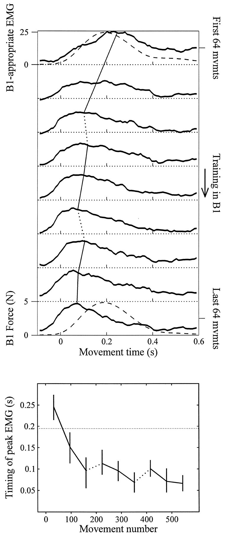
The composite EMG trace appropriate for fieldB₁ shifts with training. Top, Binned and averaged increase in the B₁-appropriate EMG trace. Each trace is averaged over 64 movements and over all 24 subjects. The progression of plots from top tobottom shows EMG traces from early to late in training. Thedashed lines in the top and bottomaxes represent the magnitude of the force created by the viscous fieldB₁, which remained consistent throughout training in B₁. Although early in training the peak of the field-appropriate EMG lagged the imposed force, with training it preceded the imposed force. The timing of the peak was estimated by a fit to a fourth-order polynomial. The best estimate of the peak and its change with training is marked by the line that crosses the EMG traces from top to bottom. In thebottom figure, the timing of the peak of the EMG traces is plotted versus movement number. The dotted lines connecting data points represent the 3 min breaks between sets. Error bars reflect 95% confidence intervals of the mean (across all 24 subjects), as determined by bootstrapping. The dotted horizontal linerepresents the timing of the peak of the force created by the force field.

With practice in the force field, the peak of theB₁-appropriate EMG trace shifted to occur earlier into the movement. To estimate the peak location of each EMG trace, the data were fitted to a fourth-order polynomial. We found that when subjects started to train in B₁, the peak of the B₁-appropriate EMG occurred 246 msec into the movement [95% CIM, (215, 274) msec]. This peak arrived 48 msec after the peak of the force created by the force fieldB₁; the peak of the robot-imposed force coincided with the peak tangential velocity of the hand and on average occurred at 195 msec into the movement throughout training inB₁. By the end of the third set of training inB₁, subjects had modified their motor commands such that the peak of the B₁-appropriate EMG occurred just 67 msec into the movement [95% CIM, (48, 86) msec; in t test of time shift, p < 1 × 10⁻⁴]. Therefore, when subjects first encountered B₁, they activated the appropriate muscles midway through the movement. The timing of this activation, coupled with the marked curvature of these movements, suggested that subjects activated these muscles through an error–driven feedback mechanism. With training in B₁, subjects learned to activate appropriate muscles earlier in the movement, in the period during which control was purely feedforward.

The changes in timing of the B₁-appropriate EMG activity revealed that subjects adapted their neuromotor output throughout all three sets of movements (Figure 6, bottom). This measure was much more sensitive than the kinematic measure of perpendicular displacement, which showed no learning during the second or third sets (compare Figure 8).

Fig. 8.

Left, Perpendicular displacement of the hand 250 msec into the movement, averaged across movement directions, during movements in null field and force field B1. Remaining plots, Rotation of a_m resultant vectors during movements in force field B₁ with respect to null field. Each point contains data from 64 movements. Eachpoint is mean and 95% confidence interval (across subjects). Dotted lines represent 3 min breaks in training.

With training, subjects generated B₁-appropriate EMG earlier in the movement. During the 3 min break between sets, however, the subjects partially unlearned this adaptation and began the next set with activation of B₁-appropriate muscles shifted later than at the end of the previous set (Figure 6,bottom). In between the second and third sets of training inB₁, this shift forward in time, i.e., the “forgetting,” was significant (mean shift, 31 msec; p < 0.05). The shift of the B₁-appropriate activation backward in time during the second and third sets and forward in time during breaks between sets indicate that the timing of this component of activation is a valid metric of learning that reveals more about the state of the adaptation than do kinematic measures alone.

Rotation of angular dependence of forces: simulation results

These results suggested that subjects initially responded toB₁ by generating appropriate EMG quite late in the movement, perhaps because of an error–feedback mechanism, but with training they learned to activate the same muscles earlier in the movement. This transition suggested that reactive responses early in training effected proactive behavior late in training. We then focused our attention on the subjects’ initial, purely feedforward, responses to the task: how do humans generate movement-initiating muscle activations based on the visual cue of a target, a desired end point of a movement? How does this neural computation, mapping stimulus to motor neuronal activation, change with learning?

To guide our investigation of feedforward muscle activation, we revisited the predicted forces generated by our ideal controller. We summarized each muscle’s force production in both the null field and in B₁ by averaging over the first 150 msec of the time series of force to create a scalar f_m. We used polar analysis (see Materials and Methods) to visualize the angular dependence of f_m (Figure7, top). We then calculated resultant vectors (radial vectors in Figure 7, top), which indicate the directions of maximal force production and summarize the dependence of force on the direction of movement. Because we predicted muscle activations using a linear transformation of muscle force, the same polar analysis reveals the predicted directional bias of the muscle activations.

Fig. 7.

Rotations in muscle-tuning curves as predicted from a computational model that assumes adaptation of an IM and tuning curves as recorded from subjects’ EMG. Top, Movement-initiating muscle forces as predicted by the model for movements in the null field (gray) and inB₁ (black). Polar plots display predicted movement-initiating force (f_m) for each direction of movement. The radii of the scale circles (centered at the origin of each plot) are 20 N. The thick vector represents a tuning curve’s resultant vector (preferred direction). The model predicts that the resultant vector should rotate between the null field and B₁. Thebars below each plot reveal the rescaling of the data (using Eq. 7 and the parameters in Table 2) into predicted muscle activations, in normalized units (nu) of EMG. Bottom, Tuning functions representing subjects’ movement initiating EMG (a_m) during training in null field (gray lines), early force field (thin black lines), and late force field (thick black lines).Thick lines are resultant vectors (preferred directions). The error bars around individual data points reflect 95% confidence intervals of the mean activation.

The simulation results revealed that by learning to compensate forB₁, the resultant vector of each muscle should rotate by a specific amount (Fig. 7, top). We found that the degree of rotation was similar over a wide range of moment arm models (Table 1) and remained constant over all levels of co-contraction. (For model C, the directions of the resultant vectors were biceps, −130.7° for null and −157.3° for B₁; triceps, 49.3° and 22.7°; anterior deltoid, 150.0° and 136.3°; posterior deltoid, −29.6° and −43.2°.) In learningB₁, the simulation predicted that the resultant vectors should rotate clockwise by 26.6° for biceps and triceps and 13–20° for anterior and posterior deltoid, depending on the moment arm model used (Table 1). These observations suggested that humans might calculate a function mapping desired end point location to initial α-motor neuronal output, and that when subjects learn to move in B₁, the activation function rotates to produce appropriate muscle forces to accurately initiate movements.

Rotation of angular dependence of EMG with training in B₁

Armed with the result that the simulated controller’s muscle activation resultant vectors rotated between the null field andB₁, we analyzed the EMG generated at the beginning of movements in both the well-learned null field and inB₁. Just as in our analysis of movements made toward 135°, we averaged each EMG trace over the period from 50 msec before through 100 msec after the beginning of the movement to create the scalar a_m. We then averaged these scalars over bins of eight movements within directions and then averaged across all subjects. We compared a_m generated at three stages of training: at the end of the set in the null field, at the beginning of the first set of training in B₁, and at the end of the third set of training inB₁. The results are shown in Fig. 7,bottom row.

In the null field (Fig. 7, gray lines), each muscle was strongly activated in certain “preferred” directions and much less activated in the opposing directions. This directional bias to the activation function was summarized by using polar analysis to construct a resultant vector for each muscle. The resultant vectors pointed toward the direction (for biceps, −130°; triceps, 50°; anterior deltoid, 127°; posterior deltoid, −17°) of maximal activity presuming a sinusoidal fit of the data.

During the first 64 movements in field B₁ (Fig.7, thin black lines), subjects began to generate movement-initiating muscle activations that differed from those generated in the null field. The resultant vectors of the a_m rotated clockwise from the directions recorded in the null field. Through the end of training in fieldB₁, the resultant vectors summarizing a_m continued to rotate in a clockwise direction (Fig. 7, bottom). To quantify this adaptation across subjects, we began by determining the orientation of individual subjects’ resultant vectors during null field andB₁ training. We rotated each subject’s activation functions so that the mean null field resultant vectors pointed toward 0°. We then calculated the mean and 95% confidence intervals of the orientations of the a_m vectors during training in the null field and B₁. The results are shown in Figure 8.

As subjects made reaching movements in the null field, the orientation of the EMG resultant vectors remained constant, and the curvature of movements remained small. In the first bin of 64 movements inB₁, subjects’ movements were markedly curved, with mean perpendicular displacement, averaged across directions, of 0.65 cm [Figure 8; 95% CIM, (0.55, 0.75) cm]. By the end of the third set of training, subjects learned to make much straighter movements [mean perpendicular displacement, −0.03 cm; 95% CIM, (−0.13, 0.07) cm; in t test of curvature reduction, p < 1 × 10⁻⁸]. The a_m resultant vectors revealed that subjects began to adapt their initial muscle activations in the first 2 min of training. In the first bin of 64 movements inB₁, the orientations of the vectors summarizing all four muscles had significantly rotated from the average null field orientations (p < 0.002 for anterior deltoid; p < 1 × 10⁻⁵ for other muscles). Although these movements were still markedly curved, subjects had begun to adapt their neuromotor output.

As subjects continued to train in B₁, the orientation of the a_m resultant vectors continued to rotate farther away from the null field orientation. By the end of the third set of training in B₁, the final directions of the a_m resultant vectors were significantly different from the orientations early in training inB₁(p < 0.05 for anterior deltoid; p < 2 × 10⁻⁵ for other muscles). The magnitudes of rotation of the a_mresultant vectors over the three sets of training inB₁ were −33.7° for biceps, −28.0° for triceps, −19.1° for anterior deltoid, and −15.6° for posterior deltoid. These observed values were similar to the predictions made by the simulated controller: within 7° for the flexors and within 2° for the extensors. This result demonstrates a technique whereby a computational model predicts the change that should occur in the activations of muscles if the brain is learning an internal model specific to a force field. The results show that the evolution of the changes in muscle activations early into the movement are reasonably close to the model’s predictions.

Activation function rotation is specific to the force field

We have suggested that subjects learned to rotate their initial muscle activations to accurately reach in the novel force fieldB₁. An alternate interpretation of our above data would be that the observed rotation was a function of either an increased familiarity with the task itself, regardless of the force field, or that the observed changes were a function of fatigue. To test these alternate hypotheses, we presented one group of eight subjects with the null field after having just completedB₁ training.

When subjects were returned to the null field (Fig.9), their hand trajectories were initially curved, in the direction opposite the error initially generated in B₁ [mean perpendicular displacement, −0.57 cm; 95% CIM, (−0.71, −0.43)]; this curvature reveals aftereffects lasting minutes after training inB₁. After two sets (350 movements) of training, however, the trajectories again resembled the straight movements made in that day’s first null field set [mean perpendicular displacement, 0.02 cm; 95% CIM, (−0.04, 0.08)].

Fig. 9.

Perpendicular displacement of the hand and rotation of a_m resultant vectors in subjects who, after training in B₁, trained in the null field 3 min later. Each point contains data from 64 movements. The first three data points are from the third set of movements in B₁. Error bars reflect 95% confidence intervals of the mean (across subjects).

As subjects made straighter movements, they generated movement-initiating muscle activations that reverted back to their original dependence on the direction of the target. Over the last two sets of training in the null field, the orientation of the a_m resultant vectors all rotated counterclockwise, back to the initial null field directions [amount of rotation: mean (95% CIM) of the amount of rotation: biceps, 26.8° (14.2°, 40.6°); triceps, 23.6° (16.8°, 29.3°); anterior deltoid, 12.3° (4.7°, 19.1°); posterior deltoid, 17.7° (15.1°, 20.4°); for all four muscles, p < 0.002]. The average resultant vectors in the last set of movements pointed in directions statistically indistinguishable from the vectors summarizing the a_m generated in the day’s first null field set (for all four muscles, p > 0.35).

The return of the orientation of the a_mresultant vectors to the original direction indicated that the rotation observed when subjects learned B₁ was not attributable to an increasing familiarity with the general task or to fatigue but reflected a force field-specific change in the neural command sent to the muscles.

Activation function rotation during training in B₂

We have suggested that the subjects may have learned to make movements in B₁ by rotating the function mapping desired end point to early muscle activation. To determine whether a different rotation of this activation function could underlie learning of other dynamic environments, we trained two groups of eight subjects each in B₂, a force field anticorrelated toB₁. One group of eight subjects completed two sets in B₂ 3 min after the three sets inB₁; the other group of eight subjects took a 6 hr break between the two force fields. In each of the subjects in these groups, we measured the a_m generated for each movement, binned the data across eight movements, and constructed resultant vectors. We then determined the orientation of these vectors compared with each subject’s initial null field orientation.

The 6 hr group had their electrodes removed after the first training session and reapplied for the second training session. Because the preferred direction of EMG is independent of the total signal strength, the resultant vector orientations calculated from the two sessions are directly comparable.

In the first 64 movements in B₂, both groups of subjects made markedly curved movements [Fig.10; across both groups, mean of perpendicular displacement, −1.64 cm; 95% CIM, (−1.45, −1.84) cm]. After two sets of training, both groups of subjects made much straighter movements [mean, −0.23 cm, 95% CIM, (−0.12, −0.34) cm]. The 3 min group, however, generated movements that were more curved than did the 6 hr group. A two-way ANOVA (two groups × six bins) revealed that the group factor is significant (F_(1,84) = 40.82; p < 1 × 10⁻⁸) and that in all but the last bin of movements, the larger amount of curvature in the 3 min group is significant (p < 0.05, Tukey test). The 3 min group initially had more difficulty than the 6 hr group in making accurate movements; this difference remained statistically significant through 10 min of training in B₂.

Fig. 10.

Perpendicular displacement and rotation of a_m resultant vectors in subjects who, after training in B₁, trained inB₂ 3 minutes (○) or 6 hr (●) later. Eachpoint contains data from 64 movements. Error bars reflect 95% confidence intervals of the mean (across subjects). The first three data points are from the third set of movements inB₁.

As both groups of subjects reduced the curvature of their movements, subjects rotated their activation functions back to and beyond the orientations appropriate for the null field. By the second set of training in B₂, all four a_m resultant vectors pointed in directions that were rotated clockwise from the activity appropriate forB₁; three of the four vectors pointed in directions significantly more clockwise than the directions appropriate for the null field [orientation of a_m vectors in the second set of B₂, mean (95% CIM): biceps, 11.8° (6.2°, 17.3°); p < 1 × 10⁻⁴; triceps, 16.9° (11.4°, 22.2°); p < 1 × 10⁻⁴; anterior deltoid, 4.1° (−9.9°, 16.3°); p > 0.5; posterior deltoid, 22.2° (17.3°, 26.8°); p < 1 × 10⁻⁴].

Although both groups produced muscle activations that rotated from the null field activity, the initial responses of the 3 min group were less adapted to B₂ than were the initial responses of the 6 hr group. The orientations of the a_mresultant vectors were compared over the three bins spanning the first set of training in B₂ (Fig. 10, open circles represent the 3 min group a_m,filled circles represent the 6 hr group a_m). We performed a two-way ANOVA (two groups × three bins) on the a_m vector orientations of biceps, triceps, and posterior deltoid. The orientations of the a_m vectors of the 3 min group had rotated significantly less than did the 6 hr group (for biceps, F_(1,42) = 5.3; p < 0.03; for triceps and posterior deltoid, F_(1,42) = 5.2; p < 0.03).

In the second set of training in B₂ (i.e., after 192 movements), the 3 min group continued to lag behind the 6 hr group in their adaptation of their activation of their posterior deltoid. A second round of two-way ANOVA on the a_mresultant vectors revealed that the posterior deltoid activation of the 3 min group was significantly closer to the orientation of the null field activation (F_(1,42) = 11.25; p < 0.002). By the second set of training inB₂, the two groups had begun to generate activations of biceps and triceps whose resultant vectors pointed in similar directions (for biceps, F_(1,42)= 0.02; for triceps, F_(1,42) = 0.43; for both, p > 0.5). Although both groups learned equally well how to appropriately control the biceps and triceps, subjects in the 3 min group continued to have added difficulty controlling their posterior deltoid appropriately.

Even though the two groups train the same amount in both force fields, the subjects with 3 min separating the two fields had more difficulty generating muscle activations appropriate to B₂. The lagging of the 3 min group suggests that the counterclockwise rotation of the activation function, that is, the internal model appropriate for B₁, had lingered in these subjects and had hampered their ability to adapt toB₂.

Anterior deltoid activation functions in the null field, B₁, and B₂

Compared with each group’s orientation in the null field, the 3 min and the 6 hr groups have different rotations of their anterior deltoid activation functions in the last set of training inB₁ (Fig. 10). The difference between the two groups stems not from differing orientations inB₁ but from differing initial orientations of anterior deltoid activation functions during the null field (Fig.11). Across the 24 subjects in all three groups, the variability of individual subject’s activation function orientation in the null field was almost three times larger for anterior than for posterior deltoid (size of 95% confidence intervals of the mean: biceps, 15.0°; triceps, 14.3°; anterior deltoid, 18.7°; posterior deltoid, 6.4°). Although the two groups of subjects had the same amount of training in the null field, the two groups generated anterior deltoid effective fields that pointed in different directions (3 min group mean, 113.7°; 6 hr group mean, 133.8°; in two-way ANOVA, two groups × three bins of movements in null field set, F_(1,42) = 6.69; p < 0.02). The differences in activations led to different movement profiles in the null field (in comparing mean perpendicular velocity traces in movements made toward 135° and 180°, mean correlation between groups, r = 0.04). Once the two groups were well trained in B₁, the anterior deltoid activation functions then pointed in similar directions (3 min group mean, 96.9°; 6 hr group mean, 100.0°; F_(1,42) = 0.04; p > 0.8), and the movement profiles of the two groups converged (135° and 180° perpendicular velocity correlation between groups, r = 0.87).

Fig. 11.

Orientations of anterior deltoid resultant vectors during training in the null field, B₁, and B₂. Whereas the previous Figures 8-10represent the rotation of a_m resultant vectors with respect to null field orientations, this figure represents the actual orientation during each stage of training. The symbols indicate the mean orientations in subjects who had a 3 min (○) or 6 hr (●) separation between B₁ andB₂. Error bars reflect 95% confidence intervals of the mean (across subjects).

When the two groups trained in their first sets of movements inB₂, the mean of the orientations of the 3 min group’s anterior deltoid activation functions rotated less toward the counterclockwise direction than did the activation functions of the 6 hr group, but the difference between the groups is marginally significant (3 min group mean, 104.8°; 6 hr group mean, 125.4°; F_(1,42) = 4.02; p < 0.055). These results suggest that despite the high subject-to-subject variation in anterior deltoid activation function orientation in the null field, the actual orientations of the anterior deltoid activation functions remained a good measure of internal model building during the learning of novel dynamics.

Reduction of wasted contraction during practice in null field and in B₁

It has been shown that as subjects learn to move their wrist against novel forces, they decrease the coincident activation of flexors and extensors, thereby decreasing the stiffness of the joint (Milner and Cloutier, 1993). To quantify how co-contraction of muscles changed during learning of multijoint reaching movements, we defined a measure of wasted contraction. We partitioned subjects’ EMG into composite traces using the simulation’s predictions of appropriate muscle activations in the null field and fieldB₁ (Table 3). For each movement, we used these coefficients to partition the four muscle traces into four direction-independent composite traces. Among these four composite traces, two pairs of traces produced forces that opposed each other. In each opposing pair, at each moment in time, the weaker of the two composite activations was cancelled by the stronger. We compared these activations to determine, in each movement, time series of wasted contraction and effective contraction.

The level of wasted contraction decreased with practice, both during training in the null field and during learning ofB₁ (Fig. 12). We averaged the time series of wasted and effective contractions in each subject across bins of 32 movements, scaled the wasted contraction as a percentage of maximum effective contraction, and then averaged these scaled wasted contractions across subjects. The peak of wasted contraction occurred ∼200 msec into the movement for all bins spanning both fields. The magnitude of the peak of wasted contraction was reduced by one-third over the course of a training set in both the null field (from 43 to 29%; p < 0.005) and the first set in B₁ (from 54 to 35%; p < 0.005). Subjects did not decrease their wasted contraction over training in the second or third sets in B₁(p > 0.5).

Fig. 12.

Wasted contraction during movements in null field and B₁. These plots show the wasted contraction (as a percent of effective contraction), averaged across subjects, as a function of time into each movement. Each line represents a bin of 32 movements. The leftmost plot contains traces from null field movements; the next three plots contain traces from the three sets of training in B₁. Thenumbers inside the plot label the wasted contraction from the first, second, and third bins of movements in each set.

During training in the null field, subjects also decreased their wasted contraction generated during the beginning of the movement, the interval over which the a_m above was calculated (average level in first bin of null, 24.5%; in last bin of null, 18.3%; p < 0.03). The mean level of early wasted contraction also changed in the first set of B₁but not significantly (p > 0.2).

Whether the robot produced a viscous force field, the maximum levels of wasted contraction occurred consistently at the midway point of the movement. Subjects reduced their peak wasted contraction when they first learned the novel force field B₁, but also, previously, when they again familiarized themselves with the well learned null field. This suggested that subjects may use wasted contraction to increase stiffness both when first regaining familiarity moving in previously learned environments and when first learning novel environments.

DISCUSSION

Subjects learned to reach in a novel viscous force field. The convergence of movements onto previous (desired) trajectories, and the existence of aftereffects when learned forces are removed, have suggested that the adaptation of an internal model underlies this learning (Shadmehr and Mussa-Ivaldi, 1994; Shadmehr and Brashers-Krug, 1997). The internal model hypothesis posits that the CNS effectively computes inverse dynamics, transforming desired trajectories into appropriate muscle activations. Here we used a simulation to predict that formation of the IM should accompany specific rotations in the directional bias of muscle activation functions. We found that the actual rotation of subjects’ spatial EMG tuning curves closely matched the predictions. The simulation also allowed us to estimate the component of muscle activation functions that produced a force that countered those in the force field. Using this transformation, we found that early in training EMG changes were driven primarily by a delayed error–feedback response. This feedback response may have formed the template for the eventual learned feedforward response.

In generating reaching movements, the CNS combines two elements of control: feedforward elements, which generate neural commands based on information available before the movement (e.g., desired trajectory); and feedback elements, which generate neural commands based on delayed visual and proprioceptive signals received during the movement. In recent computational models (Jordan, 1995; Miall, 1995; Bhushan and Shadmehr, 1999), it is assumed that feedback control provides an estimate of error, i.e., the disagreement between the actual and expected (or desired) sensory signals, and generates a delayed motor response that attempts to correct that error. Here we found that when subjects first moved in the field, their field-appropriate EMG was generated quite late in the movement, after the movement had significantly diverged from the desired trajectory. The timing of this activation relative to the perturbing force suggested that the EMG was generated by error-driven feedback control. During training, the shape of this field-appropriate EMG remained essentially invariant, but its peak gradually shifted earlier and earlier into the movement. The temporal shift culminated in a modification of the EMG pattern very early into the movement, before proprioceptive or visual information were available. This modified EMG pattern effectively predicted and canceled the upcoming pattern of imposed forces. Therefore, improvements in performance occurred as the CNS gradually incorporated the error–feedback response of the system into the feedforward command that initiated the movement.

Previous computational studies (Kawato et al., 1987; Stroeve, 1997) have shown that the motor response generated by an error–feedback system may be used to learn inverse dynamics of reaching movements. These studies suggested that a copy of the error–feedback response may be sent to the brain and then used to train the IM in a supervised learning paradigm. Our results support this general framework by showing that learning may entail an incorporation of the error–feedback response into the feedforward commands through a gradual temporal shifting process.

To investigate how gradual changes in the EMG quantitatively corresponded to IM formation, we investigated how learning an internal model should change the directional tuning of muscle activation functions. When humans make unconstrained reaching movements (or isometrically resist force), initial EMG depends on direction of movement (or imposed force) (Flanders and Soechting, 1990; Flanders, 1991; Karst and Hasan, 1991). The resulting directionally tuned function reveals, across the work space, how subjects’ internal models transform desired trajectory into muscle activations. Here we used a simple biomechanical model, which computed torque based on a dynamic IM of both the arm and the environment, to predict the shape of the tuning functions. We focused on the EMG generated between 50 msec before and 100 msec after the initiation of the movement (a_m). This period is likely to be influenced by only the feedforward component of the descending commands (Miall, 1995; Kudo and Ohtsuki, 1998), providing us with a window to the formation of the internal model.

Using this computational approach, we initially predicted the shape of the directionally tuned muscle activation functions for null field movements, with no external perturbing forces. We found that the predicted functions closely matched the measured EMG functions for the four muscles examined (Fig. 7). We summarized the directional bias of EMG functions by calculating the orientation of these functions’ resultant vectors (preferred directions). The resultant vectors remained stable as well trained subjects performed reaching movements in the null field. However, as training began in a force field, the preferred direction of each muscle’s EMG function began to rotate and eventually reached an asymptote. The internal model theory had predicted a specific rotation in each muscle’s EMG function; that prediction was confirmed. The preferred directions returned to initial conditions when the force field was removed and reversed their direction of rotation when the direction of imposed forces was reversed. These results, therefore, signified an experience-dependent adaptation of the IM. Our methods linked the computational concept of learning an internal model with changes in the directional tuning of muscle activation functions.

After training in field B₁, some subjects trained in the anticorrelated force field B₂either 3 min or 6 hr later. We had reported before that the 3 min group has much more difficulty in both their initial response and eventual adaptation to the second field (Brashers-Krug et al., 1996; Shadmehr and Brashers-Krug, 1997). Here we found that in fieldB₂, not only are the movements made by the 3 min group more disturbed than the 6 hr group, but the preferred directions of biceps, triceps, and posterior deltoid are oriented in directions more appropriate for B₁ (less appropriate forB₂) than the 6 hr group. The lingering rotations of the preferred directions provide physiological evidence that, 3 min after training, the internal model appropriate for the field just learned is still active and biasing the subjects’ ability to learn the second force field. After 6 hr have passed, the internal model no longer lingers, and subjects can learn the newest dynamics with relative ease. The results also demonstrate the robustness of the methodology in that we could compare changes in muscle activation functions despite removal and reapplication of surface electrodes in the 6 hr group.

Previous studies that have recorded EMG changes during motor learning have focused on single-joint movements and have reported increases or decreases in the magnitudes of EMG traces to demonstrate changes in neural output (Corcos et al., 1993; Gottlieb, 1994, 1996). Quantitative comparisons of these changes in magnitude with the concept of learning of an internal model are difficult because of the intrinsic variability in the strength of the signal and the difficulty in relating the absolute magnitude of EMG and generation of force. In contrast, the methods used here focus on the directional and temporal nature of the data for multijoint movements. The directional bias and the timing of the muscle activations are independent of the overall signal strength; this independence facilitates the analysis of adaptation across subjects and the quantitative comparison of EMG and computational models.

The orientation of muscle activation functions are reminiscent of the preferred direction of primary motor cortical neurons (Georgopoulos et al., 1982, 1986) in that both summarize the dependence of neuronal activity on the direction of movement. In the motor cortex, the preferred direction of some cells changes when movements are made in different postures (Sergio and Kalaska, 1997; Scott and Kalaska, 1997). A recent study has shown that the rotation of preferred direction of some cells was similar to the rotation of the directional bias of muscle activation functions (Sergio and Kalaska, 1997). Therefore, the rotation in the muscle activation functions that occurs with learning of an internal model might echo a similar change in the preferred direction of certain cortical cells. Indeed, preliminary results (Benda et al., 1997; Li et al., 1998) suggest that the tuning of select cells in a monkey’s primary motor cortex rotates when the animal learns a force field similar to the one used here.

Previous work has also shown that in making single-joint movements, subjects tend to reduce the level of co-contraction of flexors and extensors as they learn to move a novel load (Milner and Cloutier, 1993). Here we quantified co-contraction because subjects could respond to novel dynamics by simply stiffening the limb through co-contraction, rendering the arm less vulnerable to perturbations (Hogan, 1984). Therefore, one might predict that during learning of a novel task, co-activation levels should start high but decline as the internal model is acquired. Here we found that co-contraction levels (termed wasted contraction to denote the EMG that was directly cancelled by opposing activation) did significantly increase from null field to when subjects were initially exposed to the force field. With learning in the force field, the co-contraction levels declined rapidly during the initial 96 movements but remained stable with further training. The same reduction in wasted contraction, however, was also observed when subjects moved in that day’s first set in the null field, a well-learned dynamic environment. These results suggest that the CNS increases the limb’s stiffness to reduce the effect of “unmodeled dynamics” early in the learning process and reduces limb stiffness as dynamics are learned. The increased wasted contraction in the null field extends this idea to well learned dynamics; higher stiffness may facilitate the recollection of an internal model that is appropriate but stored in long-term memory.

Linking IM formation to rotation of the muscle-tuning functions raises two interesting possibilities regarding the computational organization of the internal model. First, we had previously reported that learning of a force field at a given arm configuration resulted in generalization at a new arm configuration (Shadmehr and Mussa-Ivaldi, 1994). Because learning a field at a given arm configuration results in a rotation of the muscle-tuning functions, it is possible that the magnitude of rotation is conserved when the arm must make movements at a new configuration. This would result in generalization of the force field in joint coordinates. Second, we have observed that certain force fields are much easier to learn than others. Because learning of each field is coupled to a specific rotation in the muscle-tuning functions, it is possible that the degree of difficulty in learning a field relates to how much each tuning function needs to rotate to represent that field. Further research is needed to examine whether the link between internal models and muscle tuning functions can be used to understand representation of IMs by the CNS.

REFERENCES

- 1.Atkeson CG. Learning arm kinematics and dynamics. Annu Rev Neurosci. 1989;12:157–183. doi: 10.1146/annurev.ne.12.030189.001105. [DOI] [PubMed] [Google Scholar]
- 2.Barto AG, Fagg AH, Sitkoff N, Houk JC. A cerebellar model of timing and prediction in the control of reaching. Neural Comput. 1999;11:565–594. doi: 10.1162/089976699300016575. [DOI] [PubMed] [Google Scholar]
- 3.Benda BJ, Gandolfo F, Li CSR, Tresch MC, DiLorenzo D, Bizzi E. Neuronal activities in M1 of a macaque monkey during reaching movements in a viscous force field. Soc Neurosci Abstr. 1997;23:1556. [Google Scholar]
- 4.Bhushan N, Shadmehr R. Computational architecture of human adaptive control during learning of reaching movements in force fields. Biol Cybern. 1999;81:39–60. doi: 10.1007/s004220050543. [DOI] [PubMed] [Google Scholar]
- 5.Brashers-Krug T, Shadmehr R, Bizzi E. Consolidation in human motor memory. Nature. 1996;382:252–255. doi: 10.1038/382252a0. [DOI] [PubMed] [Google Scholar]
- 6.Corcos DM, Jaric S, Agarwal GC, Gottlieb G. Principles for learning single-joint movements. I. enhanced performance by practice. Exp Brain Res. 1993;94:499–513. doi: 10.1007/BF00230208. [DOI] [PubMed] [Google Scholar]
- 7.De Luca CJ. The use of surface electromyography in biomechanics. J Appl Biomech. 1997;13:135–163. [Google Scholar]
- 8.Fisher NI. Statistical analysis of circular data. Cambridge UP; Cambridge, UK: 1993. [Google Scholar]
- 9.Flanders M. Temporal patterns of muscle activation for arm movements in three-dimensional space. J Neurosci. 1991;11:2680–2693. doi: 10.1523/JNEUROSCI.11-09-02680.1991. [DOI] [PMC free article] [PubMed] [Google Scholar]
- 10.Flanders M, Soechting JF. Arm muscle activation for static forces in three-dimensional space. J Neurophysiol. 1990;64:1818–1837. doi: 10.1152/jn.1990.64.6.1818. [DOI] [PubMed] [Google Scholar]
- 11.Flash T, Hogan N. The coordination of arm movements: an experimentally confirmed mathematical model. J Neurosci. 1985;5:1688–1703. doi: 10.1523/JNEUROSCI.05-07-01688.1985. [DOI] [PMC free article] [PubMed] [Google Scholar]
- 12.Georgopoulos AP, Kalaska JF, Caminiti R, Massey J. On the relations between the direction of two-dimensional arm movements and cell discharge in primate motor cortex. J Neurosci. 1982;2:1527–1537. doi: 10.1523/JNEUROSCI.02-11-01527.1982. [DOI] [PMC free article] [PubMed] [Google Scholar]
- 13.Georgopoulos AP, Schwartz AB, Kettner RE. Neuronal population coding of movement direction. Science. 1986;233:1416–1419. doi: 10.1126/science.3749885. [DOI] [PubMed] [Google Scholar]
- 14.Gottlieb GL. The generation of the efferent command and the importance of joint compliance in fast elbow movements. Exp Brain Res. 1994;97:545–550. doi: 10.1007/BF00241548. [DOI] [PubMed] [Google Scholar]
- 15.Gottlieb GL. On the voluntary movement of compliant (inertial-viscoelastic) loads by parcellated control mechanisms. J Neurophysiol. 1996;76:3207–3229. doi: 10.1152/jn.1996.76.5.3207. [DOI] [PubMed] [Google Scholar]
- 16.Hogan N. Adaptive control of mechanical impedance by coactivation of antagonist muscles. IEEE Trans Automatic Control. 1984;AC-29:681–690. [Google Scholar]
- 17.Jordan MI. Computational motor control. In: Gazzaniga MS, editor. The cognitive neurosciences. MIT; Boston: 1995. pp. 597–609. [Google Scholar]
- 18.Karst GM, Hasan Z. Initiation rules for planar, two-joint arm movements: agonist selection for movements throughout the work space. J Neurophysiol. 1991;66:1579–1593. doi: 10.1152/jn.1991.66.5.1579. [DOI] [PubMed] [Google Scholar]
- 19.Kawato M, Furukawa K, Suzuki R. A hierarchical neural-network model for control and learning of voluntary movement. Biol Cybern. 1987;57:169–185. doi: 10.1007/BF00364149. [DOI] [PubMed] [Google Scholar]
- 20.Kudo K, Ohtsuki T. Functional modification of agonist-antagonist electromyographic activity for rapid movement inhibition. Exp Brain Res. 1998;122:23–30. doi: 10.1007/s002210050487. [DOI] [PubMed] [Google Scholar]
- 21.Li CSR, Benda BJ, Padoa Schioppa C, Gandolfo F, DiLorenzo D, Bizzi E. Neuronal plasticity in the motor cortex of monkeys learning to adapt to a viscous force field. Soc Neurosci Abstr. 1998;24:405. [Google Scholar]
- 22.Marsden CD, Merton PA, Morton HB, Adam JER, Hallett M. Automatic and voluntary responses to muscle stretch in man. Prog Clin Neurophysiol. 1978;4:167–177. [Google Scholar]
- 23.Miall RC. Motor control, biological and theoretical. In: Arbib MA, editor. The handbook of brain theory and neural networks. MIT; Cambridge, MA: 1995. pp. 597–600. [Google Scholar]
- 24.Miall RC, Wolpert DM. Forward models for physiological motor control. Neural Networks. 1996;9:1265–1279. doi: 10.1016/s0893-6080(96)00035-4. [DOI] [PubMed] [Google Scholar]
- 25.Milner TE, Cloutier C. Compensation for mechanically unstable loading in voluntary wrist movement. Exp Brain Res. 1993;94:522–532. doi: 10.1007/BF00230210. [DOI] [PubMed] [Google Scholar]
- 26.Mussa-Ivaldi FA, Hogan N, Bizzi E. Neural, mechanical and geometric factors subserving arm posture in humans. J Neurosci. 1985;5:2732–2743. doi: 10.1523/JNEUROSCI.05-10-02732.1985. [DOI] [PMC free article] [PubMed] [Google Scholar]
- 27.Scott SH, Kalaska JF. Reaching movements with similar hand paths but different arm orientation: I. Activity of individual cells in motor cortex. J Neurophysiol. 1997;77:826–852. doi: 10.1152/jn.1997.77.2.826. [DOI] [PubMed] [Google Scholar]
- 28.Sergio LE, Kalaska JF. Systematic changes in directional tuning of motor cortex cell activity with hand location in the workspace during generation of static isometric forces in constant spatial directions. J Neurophysiol. 1997;78:1170–1174. doi: 10.1152/jn.1997.78.2.1170. [DOI] [PubMed] [Google Scholar]
- 29.Sergio LE, Kalaska JF. Changes in the temporal pattern of primary motor cortex activity in a directional isometric force versus limb movement task. J Neurophysiol. 1998;80:1577–1583. doi: 10.1152/jn.1998.80.3.1577. [DOI] [PubMed] [Google Scholar]
- 30.Shadmehr R, Brashers-Krug T. Functional stages in the formation of human long-term motor memory. J Neurosci. 1997;17:409–419. doi: 10.1523/JNEUROSCI.17-01-00409.1997. [DOI] [PMC free article] [PubMed] [Google Scholar]
- 31.Shadmehr R, Mussa-Ivaldi FA. Adaptive representation of dynamics during learning of a motor task. J Neurosci. 1994;14:3208–3224. doi: 10.1523/JNEUROSCI.14-05-03208.1994. [DOI] [PMC free article] [PubMed] [Google Scholar]
- 32.Stroeve S. A learning feedback and feedforward neuromuscular control model for two degrees of freedom human arm movements. Hum Movement Sci. 1997;16:621–651. [Google Scholar]
- 33.Thoroughman KA, Shadmehr R. Changes in EMG during learning of reaching movements. Soc Neurosci Abstr. 1998;24:419. [Google Scholar]
- 34.Wada Y, Kawato M. A neural network model for arm trajectory formation using forward and inverse dynamics models. Neural Networks. 1993;6:919–932. [Google Scholar]
- 35.Welsh AH. Aspects of statistical inference. Wiley; New York: 1996. [Google Scholar]
- 36.Wolpert DM, Ghahramani Z, Jordan MI. An internal model for sensorimotor integration. Science. 1995;269:1880–1882. doi: 10.1126/science.7569931. [DOI] [PubMed] [Google Scholar]
- 37.Wolpert DM, Miall RC, Kawato M. Internal models in the cerebellum. Trends Cognit Sci. 1998;2:338–347. doi: 10.1016/s1364-6613(98)01221-2. [DOI] [PubMed] [Google Scholar]
- 38.Wood JE, Meek SG, Jacobsen SC. Quantitation of human shoulder anatomy for prosthetic arm control—II. Anatomy matrices. J Biomech. 1989;22:309–325. doi: 10.1016/0021-9290(89)90045-6. [DOI] [PubMed] [Google Scholar]