Signal Transfer in Passive Dendrites with Nonuniform Membrane Conductance

Abstract

In recent years it became clear that dendrites possess a host of ion channels that may be distributed nonuniformly over their membrane surface. In cortical pyramids, for example, it was demonstrated that the resting membrane conductance G_m(x) is higher (the membrane is “leakier”) at distal dendritic regions than at more proximal sites. How does this spatial nonuniformity in G_m(x) affect the input–output function of the neuron? The present study aims at providing basic insights into this question. To this end, we have analytically studied the fundamental effects of membrane non-uniformity in passive cable structures.

Keeping the total membrane conductance over a given modeled structure fixed (i.e., a constant number of passive ion channels), the classical case of cables with uniform membrane conductance is contrasted with various nonuniform cases with the following general conclusions. (1) For cylindrical cables with “sealed ends,” monotonic increase in G_m(x) improves voltage transfer from the input location to the soma. The steeper the G_m(x), the larger the improvement. (2) This effect is further enhanced when the stimulation is distal and consists of a synaptic input rather than a current source. (3) Any nonuniformity in G_m(x) decreases the electrotonic length, L, of the cylinder. (4) The system time constant τ₀ is larger in the nonuniform case than in the corresponding uniform case. (5) When voltage transients relax with τ₀, the dendritic tree is not isopotential in the nonuniform case, at variance with the uniform case. The effect of membrane nonuniformity on signal transfer in reconstructed dendritic trees and on the I/f relation of the neuron is also considered, and experimental methods for assessing membrane nonuniformity in dendrites are discussed.

Transmembrane ion channels are the main carriers of electrical currents in neurons. Their type, kinetics, and spatial distribution may critically determine the properties of the electrical signals that are initiated and propagated in neurons. Importantly, these ion channels are distributed nonuniformly over the neuron surface. An obvious example is the myelinated axons where Ranvier nodes bear a high density of Na⁺ channels, whereas the internodes are bare of these channels (Hille, 1992). This spatial nonuniformity has functional implications for the propagation speed of the action potential along the axon. Ion channels are distributed nonuniformly also over the dendritic membrane. Are there some design principles that govern the distribution of channels and optimize certain aspects of signal processing in dendrites?

Early studies on excitable properties of dendrites can be found inLorente de No’ (1947), Spencer and Kandel (1961), Llinas and Sugimori (1980), and Schwindt and Crill (1995); for review, see Mel (1994). Recent experimental studies using infrared DIC video microscopy, combined with patch-clamp techniques (Stuart et al., 1993; Dodt and Zieglgansberger, 1994) directly showed that, indeed, ion channels were distributed nonuniformly over the dendritic surface (for review, seeJohnston et al., 1996). Recordings from membrane patches, excised from the apical trunk of hippocampal CA1 pyramidal neurons, showed that both the A-type and the delayed rectifier K⁺ conductances linearly increased with the distance from the soma (Hoffman et al., 1997). The density of I_h currents also increase in these cells (Magee, 1998). An increase in the density of both I_h current and the cesium-insensitive membrane conductance at distal dendritic regions was also recently observed in neocortical layer V pyramids (Stuart and Spruston, 1998). Nonuniformity in dendritic excitability was also found in other neuron types (Stuart and Häusser, 1994; Turrigiano et al., 1995; Bischofberger and Jonas, 1997; Kavalali et al., 1997; for review, see Segev and Rall, 1998).

Spatial distribution and spatiotemporal activation pattern of transmitter-gated conductances may also cause nonuniformity of the dendritic membrane. Thus, the dendritic membrane conductance is expected to develop time- and activity-dependent spatial heterogeneities (Holmes and Woody, 1989).

Most of our intuitions regarding how the interplay between dendritic morphology, physiology, and input conditions determine the input–output properties of dendrites rely on Rall’s cable theory. In this framework, the effect of geometric nonuniformities in the dendritic tree, including tapering and branching, was analyzed (Butz and Cowan, 1974; Horwitz, 1981, 1983; Poznanski, 1988; Schierwagen, 1989; Abbott, 1992; Holmes et al., 1992; Holmes and Rall, 1992a,b;Agmon-Snir and Segev, 1993; Major et al., 1993a–c; Segev et al., 1995;Rall and Agmon-Snir, 1998), and the impact of nonlinear voltage- and transmitter-gated dendritic ion channels, as well as of massive synaptic input on the input–output properties of neurons, was explored theoretically (Barrett and Crill, 1974; Shepherd et al., 1985; Miller et al., 1985; Fleshman et al., 1988; Segev and Rall, 1988; Clements and Redman, 1989; Holmes, 1989; Bernander et al., 1991; Rapp et al., 1992;Siegel et al., 1994; Bernander et al., 1994; De Schutter and Bower, 1994; Pinsky and Rinzel, 1994; Schwindt and Crill, 1995; Stuart and Sakmann, 1995; Wilson, 1995; Mainen and Sejnowski, 1996). A review of these issues can be found in Koch (1999). Experimental studies on the input–output properties of nonlinear dendrites can be found in Laurent et al. (1993), Nicoll et al. (1993), Haag and Borst (1996), and Chen et al. (1997). However, there is yet no systematic study on the effect of membrane nonuniformity in dendrites, although previous studies did consider the possibility that the soma membrane is leakier than the dendritic membrane (Rall, 1962; Rall and Shepherd, 1968; Iansek and Redman, 1973; Durand, 1984; Kawato, 1984; Major et al., 1993a).

Motivated by the recent experimental evidence about membrane nonuniformity in dendrites, the present study explores, using analytical tools, whether there is some functional advantage of membrane nonuniformity for the transfer of synaptic signals from the dendrites to the soma. In the tradition of W. Rall, we treat here, as a first stage, the case in which the dendritic membrane conductance G_m(x) is spatially nonuniform and passive. All mathematical considerations are grouped in the Appendixes (on-line at www.jneurosci.org).

MATERIALS AND METHODS

The cable equation (Rall, 1959) away from current sources for a passive cylinder with nonuniform membrane conductance is:

$${\lambda }^2(x)\frac{{\partial }^{2}V}{\partial x^2}-{\tau }_{\text{m}}(x)\frac{\partial V}{\partial t}-V=0,$$ Equation 1

where τ_m(x) = C_m/G_m(x) is the (variable) passive membrane time constant and λ(x) = $\sqrt{\text{d}/(4G_{\text{m}}(\text{x})R_{\text{i}})}$is the (variable) space constant, G_m(x) is the specific membrane conductance, and d is the diameter of the cylinder. In the uniform case, in which G_m(x) is constant, λ(x) = λ^u, and τ_m(x) = τ_m^u; the superscript, “u” is used throughout this work to label the uniform case. These and other quantities are defined in Table1.

Table 1.

Table of symbols

V	Transmembrane voltage (relative to resting potential)	mV
d	Diameter of the dendritic cylinder	cm
ℓ	Length of the dendritic cylinder	cm
x	Physical distance from the origin (usually the soma)	cm
Gm(x)	Specific membrane conductance	S/cm2
Gm = 1/ℓ ∫0ℓGm(x)dx	Average membrane conductance	S/cm2
γm(x) = Gm(x)/ Gm	Dimensionless membrane conductance	Dimensionless
Rm(x)	Specific membrane resistance	Ωcm2
Ri	Specific cytoplasm resistivity	Ωcm
ri = 4Ri/(πd2)	Internal resistance per unit length of cylinder	Ω/cm
Cm	Specific membrane capacitance	F /cm2
α	Slope parameter (−1 ≤ α ≤ 1)	Dimensionless
λ(x) = $\sqrt{\text{d}/4G_{\text{m}}(\text{x})R_{\text{i}}}$	Space constant (nonuniform case)	cm
λu = $\sqrt{\text{d}/4{\overline{G}}_{\text{m}}{R}_{\text{i}}}$	Space constant (uniform case)	cm
L = ∫0ℓ dx/λ(x)	Generalized electrotonic length	Dimensionless
Lu = ℓ/λu	Electrotonic length (uniform case)	Dimensionless
Xu = x/λu	Distance from location x to origin, in units of the uniform space constant	Dimensionless
Rin(x)	Input resistance at location x	Ω
Gin(x) = 1/Rin(x)	Input conductance at location x	S
Rx,y	Transfer resistance from location x to location y	Ω
Ia	Axial current	A
G∞u = (π/2) $\sqrt{{\overline{G}}_{\text{m}}{\text{d}}^3/R_{\text{i}}}$	Input conductance of a semi-infinite uniform cylinder	S
GL	Axial leak conductance at boundary	S
B = GL/G∞u	Boundary condition	Dimensionless
τm(x) = Cm/Gm(x)	Local membrane time constant	sec
τmu = Cm/ Gm	Membrane time constant (uniform case)	sec
τnu, τns	n -th equalizing time constant (uniform and slope case, respectively)	sec
δ(x), δ(t )	Delta function
𝒢 (x, y, t)	Green function
gsyn	Synaptic conductance	S
Esyn	Synaptic reversal potential	mV

To understand the effects of different G_m(x) functions, we need to impose some constraint that will allow us to compare these G_m(x) functions. The most natural assumption is that the total membrane conductance of the cable is preserved in all cases:

$$\pi d\underset{0}{\overset{\ell }{\int }} G_{\text{m}}(x)\text{dx}=\text{const}.$$ Equation 2

This implies that there is a fixed number of (passive) ion channels in the modeled structure and that these channels are allocated to different regions of the cable, depending on the shape of G_m(x).

The case of membrane nonuniformity that will gain the main focus of the present work is the slope case, in which G_m(x) linearly increases with the distance from the “soma” (x = 0), namely, G_m(x) = ax + b. This case has received some recent experimental support (Hoffman et al., 1997). All quantities are labeled, in this case, with the superscript “s.” In the case of cylinder of length ℓ, the constraint of a fixed total conductance, Equation 2, implies that:

$$G_{\text{m}}^{\text{s}}(x)={\overline{G}}_{\text{m}}\left(1+2\alpha \frac{x-\ell /2}{\ell }\right),$$ Equation 3

where G_m is the average membrane conductance over the membrane area, x is the location along the cylinder (0 ≤ x ≤ ℓ), and the dimensionless parameter α = aℓ/(2 G_m) is the slope a in units of 2 G_m/ℓ. Because G_m(x) should be positive for all x, α is bounded, −1 ≤ α ≤ 1. The uniform case is obtained when α = 0, whereas for the case of maximal slope, α = 1. In this case, the membrane conductance increases from 0 at x = 0 to a maximum of 2 G_m at x = ℓ.

For DC current injection, the membrane voltage (away from current sources) satisfies the steady-state cable equation:

$${\lambda }^2(x)\frac{d^{2}V}{{\text{dx}}^2}-V=0.$$ Equation 4

Equation 4 can be analytically solved for several nonuniform conductance profiles. The solutions for typical increasing of G_m(x) functions (power law, exponential, etc.) are given in Appendix B; they all involve special functions (Abramowitz and Stegun, 1970). Mathematica software (Wolfram, 1991) was used for numerical evaluations of these analytical solutions; transient simulations and computations of transfer resistances in reconstructed dendrites were implemented using NEURON simulator (Hines and Carnevale, 1997).

The transient voltage–response of a cable with nonuniform membrane conductance can be computed using the Green function, 𝒢(x, y, t), of the problem which satisfies:

$$({\lambda }^{\text{u}}{)}^2 \frac{{\partial }^2\mathcal{G}(x,y,t)}{\partial x^2}-{\tau }_{\text{m}}^{\text{u}} \frac{\partial \mathcal{G}(x,y,t)}{\partial t}-\frac{G_{\text{m}}(x)}{{\overline{G}}_{\text{m}}} \mathcal{G}(x,y,t)=-\delta (x-y)\delta (t),$$

together with the imposed boundary and initial conditions. Separating time and space variables, the Green function can be expressed as an orthonormal expansion (Rall, 1969):

$$\mathcal{G}(x,y,t)=\sum _{j=0}^{\infty } c_{\text{j}}{\mathcal{G}}_{\text{j}}(x){\mathcal{G}}_{\text{j}}(y)e^{-t/\tau j},$$

where the basis functions 𝒢_j satisfy:

$$\frac{1}{\ell } \underset{0}{\overset{\ell }{\int }} {\mathcal{G}}_{\text{j}}(x){\mathcal{G}}_{\text{k}}(x)\text{dx}=\left\{\begin{array}{cc}1& j=k\\ 0& j\ne k\end{array}\right..$$

The system time constant τ₀ and the equalizing time constants τ_j (j ≥ 1), together with the associated eigenfunctions 𝒢_j (j ≥ 0), are obtained by solving the eigenvalue problem:

$$({\lambda }^{\text{u}}{)}^2 \frac{d^2{\mathcal{G}}_{\text{j}}(x)}{{\text{dx}}^2}-\left(\frac{G_{\text{m}}(x)}{{\overline{G}}_{\text{m}}}-\frac{{\tau }_{\text{m}}^{\text{u}}}{{\tau }_{\text{j}}}\right){\mathcal{G}}_{\text{j}}(x)=0,$$ Equation 5

with imposed boundary conditions at x = 0 and x = ℓ. It is meaningful to distinguish τ₀ from the other time constants (Rall, 1969). Indeed, τ₀ governs the slow relaxation of the voltage at large t, and for uniform cables with sealed ends, τ₀ = τ_m^u. The other, smaller time constants control the faster spatial equalization of voltage gradients, and they vanish in the limit of extremely compact cables (L^u → 0). As shown in Appendix E, the eigenvalue problem is analytically tractable in the slope case: the eigenvalues are determined by solving a transcendental equation, and the associated eigenfunctions can be expressed as linear combinations of Airy functions.

The eigenvalue Equation 5 is formally identical to the Schrödinger eigenvalue problem for the one-dimensional bounded motion of a particle in quantum mechanics (Landau and Lifschitz, 1997). This analogy, which is elaborated on in Appendix D.1, is useful because it provides a visual representation of the Green function of the cable problem in terms of discrete energy states in a potential well. It provides new insight on how the system time constant and the equalizing time constants, together with the associated eigenfunctions, depend on the membrane conductance profile and on other cable parameters such as the electrotonic length. Note also that another representation of the Green function, as a diffusion process, was proposed by Abbott et al. (1991), Abbott (1992), and Bressloff and Taylor (1993); this approach also relies on concepts and methods (i.e., path integrals or their discrete counterpart) that were previously introduced in physics. These methods can be applied to any profile of nonuniform specific conductance on the dendritic tree, but they require the numerical evaluation of the contributions of many paths. This limits its practical usefulness mostly to the accurate estimation of the short-term transient behavior. In contrast, our approach is limited to certain types of conductance profiles, but it provides analytical results and enables us to accurately determine, through the computation of the larger time constants, how the slow relaxation of transients proceeds.

RESULTS

Steady current input in nonuniform cylinders

The steady-state voltage profile along a cylinder with both ends sealed, following constant current injection at different locations, is shown in Figure 1A for the uniform case and the maximal slope case (α = 1). This figure shows that the voltage at x = 0 (soma) is always larger in the slope case, even when the local voltage response at the input site is smaller than in the uniform case (e.g., at the distal end where x = ℓ = 1000 μm). As demonstrated in Figure1B, the voltage attenuation between any input point x and the soma is smaller in the slope case. Note that this figure also describes the attenuation of the time integral of the potential in the case of transient current injection (Rall and Rinzel, 1973). Thus, distributing the same total membrane conductance nonuniformly rather than uniformly improves the voltage response at the soma.

Fig. 1.

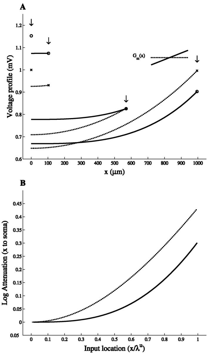
Voltage attenuation is smaller in the slope case than in the uniform case. A, Voltage profiles for a DC current injection at x = 0, 100, 570, and 1000 μm in the uniform case (dotted line) and the maximal slope case (continuous line; see inset). Voltage response at input locations (arrows) is marked by circles in the uniform case and by crosses in the slope case. Cable parameters are ℓ = 1000 μm, d = 4 μm, R_i = 200 Ωcm, R_m^u = 20,000 Ωcm², and L^u = 1 (the slope per unit length in the maximal slope case is 1E−5(S/ cm²)/100 μm). The value of the DC current is chosen so that the local voltage–response to current injection at x = 0 is 1 mV in the uniform case.B, Log voltage attenuation, LA_x,0 = ln (V(x)/V(x = 0)), from the input site, x, to x = 0.

To characterize the effect of steady current injection at point x on the voltage response at the soma, the transfer resistance R_x,0 = V(0)/I(x) is used. Figure 2A shows the normalized transfer resistance between the input location and the soma for cylinders of different electrotonic length. In the maximal slope case, the transfer resistance is always larger (for every x) than in the corresponding uniform case, and thus for all input locations the voltage response at the soma is larger when the conductance linearly increases in the cylinder. This property is independent of the cylinder physical length. The difference between the two cases grows with the electrotonic length of the cylinder. It is also true for all the intermediate linear slopes (i.e., 0 < α ≤ 1).

Fig. 2.

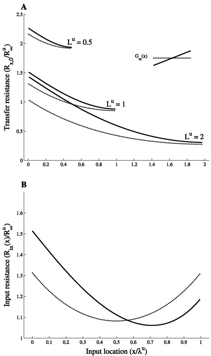
Voltage transfer is enhanced in cables with nonuniform membrane conductance. A, Transfer resistance, R_x,0, from input location x to the soma (x = 0). The results are shown for three cylinders (L^u = 0.5, 1, and 2, respectively) in the uniform case (dotted lines) and the slope case (solid lines). B, Input resistance, R_in, versus input location for the uniform case (dotted line) and the slope case (solid line). L^u = 1. Note that both R_x,0 and R_in are normalized by R_∞^u, the input resistance of the uniform cylinder when extended to be semi-infinite. As shown byRall (1959), uniform cylinders with the same L value but with different specific properties have the same transfer resistance, R_X,0, when each cylinder is normalized by its corresponding R_∞ value. This also holds true for cylinders with linearly increasing membrane conductance, if the slope parameter α and the electrotonic length L^u of the corresponding uniform cylinder are the same for all cylinders considered. The normalizing factor is then the input resistance R_∞^u of the semi-infinite uniform cylinder of specific conductance G_m^u = G_m.

Figure 2B shows the normalized input resistance R_in(x) = R_x,xfor cylinders with electrotonic length L^u = 1. In the uniform case, R_in(x) is symmetric with respect to the midpoint x = ℓ/2, where the minimum is obtained. This is no longer true in the maximal slope case in which R_in(x) is larger in the proximal part of the cylinder and smaller in its distal part compared with the uniform case. This is expected because, in the slope case, the membrane is “leakier” in distal regions of the cylinder. Because R_in is determined not only by the local membrane conductance but also by the cable properties and the boundary conditions, the intersection between R_in(x) in the two cases is not at the cylinder’s midpoint, X^u = 0.5 (where G_m^s(x) = G_m^u), but rather at X^u ≃ 0.57. A given current input at X^u > 0.57 will result in a smaller local voltage response in the slope case because of the smaller input resistance in these sites compared with that of the uniform case. Nevertheless, the resultant voltage at the soma is larger in the slope case because of the larger transfer resistance in this case. In contrast, for all X^u < 0.57, both R_in and R_x,0 are larger in the slope case, giving rise to a larger voltage response both locally and at the soma. The “benefit,” in terms of the relative increase of the soma voltage, gained from having a maximal slope conductance rather than a uniform conductance ranges from 3% for distal inputs to 16% for proximal inputs in cylinders with electrotonic length, L^u = 1 (see Fig. 4B, current input).

Fig. 4.

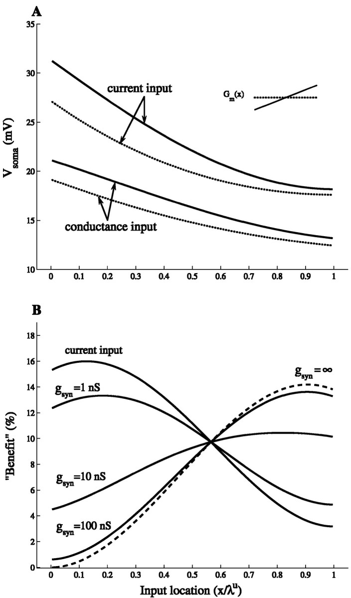
Distal synaptic inputs are more efficient when G_m(x) linearly increases with distance. A, Soma voltage as a function of input location in the cylinder for both a steady-state synaptic conductance change (g_syn = 2 nS, E_syn = 65 mV; bottom two curves) and for a DC current injection (I = g_synE_syn; top two curves). The uniform case (dotted line) and the maximal slope case (continuous line) are shown; cable properties are as in Figure 1A. B, The relative increase in soma voltage, (V_soma^s − V_soma^u)/V_soma^u, denoted as “Benefit,” attributable to the spatial gradient in the membrane conductance, is displayed as a function of input location. Current injection and three cases of steady-state synaptic conductance change (g_syn = 1, 10, and 100 nS) are shown as a function of input location. The dashed curvecorresponds to the limiting case in which g_syn→ ∞. This curve was computed by taking the limit, g_syn → ∞, in Equation 6. The relative increase in soma voltage is then given by (AF_x,0^u − AF_x,0^s)/AF_x,0^s. This can be interpreted as the benefit attributable to the difference in the attenuation factor. This is reasonable because, in this limit, the local voltage is E_syn in both the slope and the uniform cases, and only the difference in AF_x,0causes a difference in soma voltage. (Note that in this limit, the soma voltage is inversely proportional to the attenuation factor.)

The focus in the above analysis was on the slope case, in which G_m(x) is a linear function of x, and more specifically on the limiting case where α = 1. In Figure 3, the transfer resistance for several power law functions of G_m(x) with increasing exponent (0, 1/2, 1, and 2) is computed. All cases with integer power are actually analytically tractable (see Appendix B.2). G_m(x) is normalized such that the constraint of a fixed average membrane conductance (Eq. 2) holds, and in all nonuniform cases, G_m(0) = 0. Figure 3 shows that, compared with the uniform case, the transfer resistance is always increased by a gradient of membrane conductance, and the difference compared with the uniform case increases with the steepness of the conductance profile. Indeed, when G_m(x) increases with an exponent of 2, the benefit, in terms of the relative increase of the soma voltage, ranges from 6% for distal inputs to 26% at more proximal sites, with an average of 17%. Note also that because of the reciprocity property of the transfer resistance [R_x,y = R_y,x (Koch, 1999)], the effect of spatially decreasing conductance profiles can be deduced from these results (see Appendix C.3).

Fig. 3.

Transfer resistance increases with the steepness of G_m(x). Transfer resistance is plotted for a cylinder of length L^u= 1 for different conductance profiles; uniform, G_m(x) = G_m (dotted line); square root, G_m(x) = G_m (3/2 $\sqrt{\text{x}/\ell }$) (dotted–dashed line); linear, G_m(x) = G_m(2x/ℓ) (continuous line); square, G_m(x) = G_m(3(x/ℓ)²) (dashed line). The corresponding G_m(x) functions are drawn in theinset.

Finally, we note that the generalized electrotonic length of a given cylinder, L = ∫₀^ℓ dx/λ(x), is smaller for the slope case compared with the uniform case. Indeed, for the slope case, L is given by:

$$L=L^{\text{u}} \frac{((1+\Vert \alpha \Vert {)}^{3/2}-(1-\Vert \alpha \Vert {)}^{3/2})}{3\Vert \alpha \Vert }.$$

L decreases with increasing ‖α‖ and reaches its minimum, L = $\sqrt{8/9}$L^u, for α = ±1. More generally, Appendix A.1 shows that any membrane conductance heterogeneity decreases L in comparison with the corresponding uniform case, making the cable electrotonically more compact. However, this does not necessarily imply that voltage attenuation is reduced in these more compact cables (see Discussion).

Synapses as input

Realistic synaptic inputs involve conductance changes, which implies that the synaptic current nonlinearly depends on the synaptic conductance change g_syn. The difference in input resistance between the slope and the uniform case (Fig.2B) leads to a different degree of local voltage saturation in these two cases, and consequently, to differences in the amount of current generated by the synapse.

The voltage response at x = 0, attributable to the steady-state activation of a synapse at location x is:

$$V(0)=g_{\text{syn}}{E}_{\text{syn}} \left(\frac{G_{\text{in}}(x)}{g_{\text{syn}}+G_{\text{in}}(x)}\right) R_{\text{x},0},$$ Equation 6

where E_syn is the reversal potential of the synaptic current, and G_in(x) = 1/R_in(x) is the input conductance at location x before the activation of the synapse, as computed in Figure 2B. Note that the right side of the equation is simply composed of the local input current produced by the synapse, multiplied by the transfer resistance from the input site to the soma. The derivation of this equation is given in Appendix C.2.

Figure 4A shows the voltage at x = 0 in response to the steady-state activation of an excitatory synapse in the maximal slope case and the uniform case (bottom two curves). As a reference, the voltage response to a DC current input, I = g_synE_syn, is also shown (top two curves). This is the current that the synapse would generate if the synaptic current were not limited by saturation, and this is, therefore, the upper bound on the synaptic current that is actually generated. The corresponding curves are then proportional to R_x,0 (compare with Fig. 2A). As expected from synaptic saturation, V(0) in both the uniform case and slope case is smaller for the conductance input case compared with the corresponding current input case. Still, as for the current input, the soma voltage is larger in the slope case for all input locations (Fig. 4A, two bottom curves). To highlight the effect of the nonuniform membrane conductance in the case of synaptic inputs, we have plotted in Figure4B the benefit (the relative change in the soma voltage) of having a maximal slope membrane conductance rather than a uniform membrane conductance. The reference case of a DC current input, I = g_synE_syn, is also shown (current input curve); the corresponding curve is independent of g_syn(because of linearity) and is given by (R_x,0^s − R_x,0^u)/R_x,0^u.

All of the curves in Figure 4B intersect at X^u ≃ 0.57. At this site, the input resistance in the slope case is the same as in the uniform case (Fig.2B), and the difference between the two cases (which is also independent of g_syn) is attributable only to differences in the transfer resistance, R_x,0 (Eq. 6). Most notable is that the relative change in the soma voltage is always positive (and is independent of E_syn). This means that when the input is a synaptic conductance change, the nonuniformity in the membrane conductance results in an increase of the soma voltage compared with the uniform case, as was also the case for current input. For input locations more distal than the point of intersection, the current input case sets a lower bound for this effect, and the benefit of having a slope membrane conductance grows with increasing g_syn, eventually reaching a limit (Fig.4B, dashed curve). In contrast, for proximal input locations, the current input case sets an upper bound for the effect of the slope membrane conductance. The benefit of having a slope conductance is smaller when the input is a synapse rather than a current input, and this benefit decreases with increasing g_syn.

These results can be explained as follows. First, in the slope case, more synaptic current is generated at leakier distal inputs sites because the local voltage saturation is reduced as a result of the lower input resistance at these sites (Fig. 2B). The opposite is true for proximal input sites. Second, the transfer resistance is always larger in the slope case compared with the corresponding uniform case (Fig. 2A). All in all, distal synaptic inputs benefit twice from having slope membrane conductance. For proximal synaptic inputs, however, there is a competition between the reduction of the synaptic current on the one hand (caused by stronger saturation) and the increase in the transfer resistance on the other hand. Because the latter dominates, synapses are always more effective in producing a larger soma voltage when G_m linearly increases with distance. Distal synapses can exploit this membrane nonuniformity more effectively, because of a decreased synaptic saturation, than do proximal synapses. As a consequence, the largest relative benefit is obtained for weak proximal synapses and for strong distal synapses.

Dendritic trees

The previous sections dealt with cylinders of constant diameter with both ends “sealed.” There are two main difficulties in extending the insights gained in these sections to dendritic trees with realistic geometries. The first arises from the “sealed ends” assumption and the second from the assumption of constant diameter. Real dendrites are complex branching structures with frequent changes in diameters, and although sealed end boundary condition is usually accepted for the termination of distal dendritic arbors, this condition is generally inappropriate at the proximal end of dendrites, toward which the synaptic current flows. At this end, the impedance load attributable to the soma and the other dendritic trees emerging from it may result in “leaky” boundary conditions. In the following, we will separately deal with each of these issues and then explore their interplay by considering relevant models of reconstructed neurons.

Boundary conditions

When the synaptic current flows from the “input dendrite” toward the soma, the steady-state boundary condition at the soma is given by the leak conductance, G_L, which is the sum of the individual input conductances of all the other dendrites, each taken alone, plus the input conductance of the somatic membrane (Rall, 1959). The “leakiness” of the boundary condition can then be quantified by the parameter B = G_L/G_∞, where G_∞ is the input conductance of a semi-infinite cylinder with the same diameter and specific properties as the “input” dendrite. B = 0 is the sealed end boundary condition (no leak through the termination), and B = ∞ is the “killed end” condition. Large B values indicate a large “leak” at the boundary.

In Table 2, B was computed for three reconstructed dendritic trees shown in Figure 7, assuming uniform membrane resistance of 20,000 Ωcm² (fourth column) and 50,000 Ωcm² (fifth column). The values obtained span two orders of magnitude, from 0.1 (in Purkinje cells) to more than 10 for the (thin) basal dendrites of hippocampal and neocortical pyramidal cells. For these basal dendrites, the soma and all other dendrites impose a large conductance load. The boundary conditions for the apical tree of these two cells are less leaky.

Table 2.

Boundary condition (B) at the soma for the dendritic trees in Figure 7

Cell type	Dendrite	B20,000	B50,000	d (μm)	max L20,000u
Layer V pyramidal	Apical	0.96	0.47	8.4	2.6
	Basal (n = 10)	12.1  ± 8.7	6.7  ± 4.8	2.5  ± 1	0.66
Hippocampal CA1	Apical	1.6	1.1	2.75	3.65
	Basal (n = 6)	8.3  ± 4.4	6.2  ± 3.2	1.3  ± 0.6	1.7
Cerebellar Purkinje		0.11	0.07	7.2	0.36

B values were computed at the point of connection between the soma and the dendrite indicated (e.g., the apical dendrite). Computations were performed assuming uniform R_m^u of 20,000 Ωcm²(third column) or 50,000 Ωcm² (fourth column). In both cases R_i = 200 Ωcm. For each dendrite B = (2/π) $\sqrt{R_{\text{m}}{R}_{\text{i}}}$d₀^−3/2/R^*_in, where d₀ is the diameter of the dendrite at the connection point with the soma (fifth column), and R^*_in is the input resistance of the neuron at the soma when the dendrite is removed. The last column denotes the longest electrotonic path, from the soma to a dendritic terminal, for the uniform case (R_m^u = 20,000 Ωcm²).

Fig. 7.

Voltage transfer is enhanced in dendritic trees with slope membrane conductance. Transfer resistance in the slope case and the uniform case for three reconstructed trees: A, cerebellar Purkinje cell (provided by M. Rapp, Hebrew University);B, D, layer V neocortical pyramidal cell (provided by J. C. Anderson, K. A. C. Martin, and R. J. Douglas, ETH, Zurich); C, hippocampal CA1 cell (provided by D. Turner, Duke University). D, Same as B but now the total conductances of the apical tree and of the basal dendrites both retain separately in the slope case the values they have in the uniform case. In A–C , the constraint of a fixed total membrane conductance in slope and uniform cases was imposed for the whole dendritic arborization. In all four cases G_m^u = 20,000 S/cm² and R_i = 200 Ωcm. To keep the constraint of a fixed total membrane conductance, a slope of 2.5E−5(S/ cm²)/100 μm was used inA, 1.5E−5(S/ cm²)/100 μm inB, and 8.6E−6(S/ cm²)/100 μm in C. In D a slope of 9.2E−6(S/ cm²)/100 μm was used for the apical dendrite, and a slope of 4.5E−5(S/ cm²)/100 μm was used for all the basal dendrites. Scale bar, 100 μm.

How do leaky boundary conditions affect the results obtained thus far? Figure 5A depicts the effect of varying boundary conditions at x = 0 on the transfer resistance R_x,0. When the proximal termination becomes leaky (B ≈ 1), the transfer resistance curves in the uniform case and in the slope case intersect; the intersection point moves closer to the proximal end as B increases. In contrast to the sealed end case, in these cases distal current input gives rise to a smaller somatic voltage in the slope case compared with the uniform case.

Fig. 5.

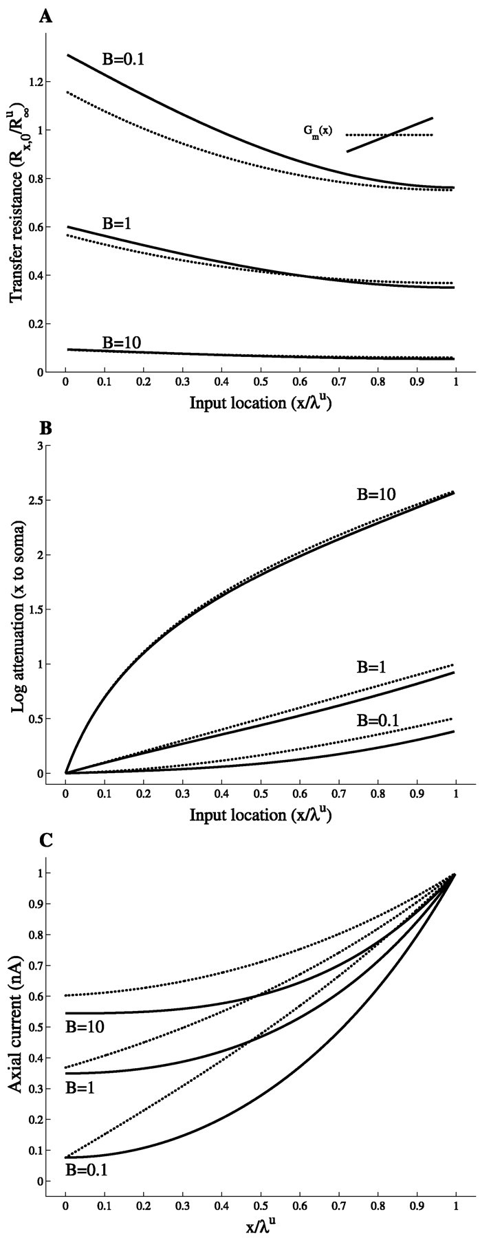
Leaky boundary conditions reduce the effects of membrane nonuniformity. A, Transfer resistance R_x,0(x); B, log voltage attenuation (LA_x,0); C, axial current along the cylinder in response to a DC current injection at x = ℓ. Results are displayed for a cylinder of length L^u = 1, with “sealed end” at x = ℓ and for three different boundary conditions at x = 0 (B = 0.1, B = 1, and B = 10). Both the uniform case (dotted lines) and the slope case (solid lines) are shown.

The attenuation factor, however, remains smaller in the slope case (Fig. 5B), even with large B value, although the difference between the two cases progressively diminishes as the leakiness at the termination increases. The results of Figure 5A, B demonstrate that, with increasing B values, the longitudinal current flow in the cylinder becomes more and more dominated by the leakiness at the boundary. Consequently, the effects of the membrane nonuniformity become progressively less significant. This effect is further demonstrated in Figure 5C. Here a DC current is injected to the distal end of the cylinder, and the axial current I_a (given by −1/r_i ∂V/∂x) is plotted as a function of x for three boundary conditions. First, notice that in both cases (slope and uniform), the larger the B value, the larger is the axial current I_a. Note also that the axial current in the slope case is everywhere smaller than in the corresponding uniform case. This is true for this specific distal input location and is the result of the larger current loss (shunt) through the leakier distal membrane in the slope case. One may erroneously conclude from this figure that the charge transfer from x to the soma (x = 0) is always smaller in the slope case for all input locations and boundary conditions. However, for many input locations, V_soma is larger in the slope case (Fig. 5A), which implies that the charge transfer to the soma is then larger than in the uniform case. This is true because I_a(soma) = V_somaG_L, and G_L is the same in the uniform case and the slope case (same B value). Hence, the charge that reaches the soma can be easily derived by scaling Figure 5A by the appropriate G_L value that corresponds to a given value of B. Then, for a given B value and input location x, the axial current that reaches the soma is larger in the slope case if R_x,0^s > R_x,0^u.

In the figure above we imposed the same leak conductance (G_L) at the boundary for both the slope case and the uniform case. However, if we impose the slope condition on a realistic dendritic tree, we expect that for each dendrite, B will be different from its value in the corresponding uniform case. This is because the input resistance at the somatic end is increased in the slope case compared with the corresponding uniform case (Fig. 2), and thus G_in into this dendrite is decreased. This decreases G_L for all the other dendrites (and thus the B value becomes smaller). Note that Figure 5A also shows that in both the uniform and slope cases, the smaller B is, the better the voltage transfer from the dendrites to the soma. This means that a dendrite with a slope conductance gradient will impose a lesser conductance load to the other dendrites stemming from the soma, compared with a dendrite with uniform membrane conductance. Signal transfer from these other dendrites to the soma will then be improved because the boundary condition at their somatic end will be less leaky. To assess what are the effects of this interplay between conductance gradients and boundary conditions, it is necessary to consider reconstructed neurons (see below).

Branching

The results derived above for cylinders cannot be readily extended to branching structures. Consider the simple case of a branched cable consisting of a father branch and two daughter branches, one thick and one thin, such that this structure is equivalent to a single cylinder in the uniform case (Rall, 1959). This implies that the thick daughter branch is physically longer than the thin daughter branch. Now consider the maximal slope case in which the specific membrane conductance increases with a constant slope per unit length from the proximal end of the father branch to the distal terminals of the daughter branches. This case is analytically handled in Appendix A.2 and illustrated in Figure 6. Because the thin branch is physically shorter (and the conductance is growing as a function of distance from the soma), the total membrane conductance in this thin and shorter branch is smaller than in the thicker sibling branch, and the membrane at its termination is less leaky. Indeed, most of the membrane conductance is now allocated to the thick branch.

Fig. 6.

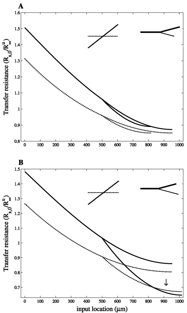
Signal transfer in nonuniform branching geometries. Transfer resistance R_x,0 is plotted as a function of input location, x, in a branched structure. The uniform case (dotted lines) and the maximal slope case (continuous line), in which G_m(x) linearly increases with the same slope along all the branches, are shown. The geometry of the branched structure (inset) is as follows. A, ℓ = 500 μm and d = 4 μm for the father branch; for the thin daughter branch, ℓ = 316 μm, d = 1.6 μm, and for the thick daughter branch, ℓ = 453 μm, d = 3.3 μm. In the uniform case this structure is equivalent to a single cylinder of length L^u = 1.B, Same as in A, but the thin daughter branch is 200 μm longer (see inset). In both A andB the constraint of a fixed total membrane conductance (Eq.2) was imposed. This yields a slope conductance of 1.042E−5(S/ cm²)/100 μm in caseA and 0.967E−5(S/ cm²)/100 μm in case B.

One consequence of this asymmetry in the allocation of ion channels is that the branched structure is no longer equivalent to a single cylinder in the slope case; the thin branch is now electrically shorter than the thick branch. Another consequence is that the total conductance along a given path from the soma to some terminal is not the same in the uniform case and the nonuniform case. Thus, when comparing the electrotonic properties of this structure between the uniform and slope case, the insights gained from a single cylinder are not directly valid because the constraint of the total amount of conductance imposed on the whole structure is not satisfied for each path separately.

Because of the asymmetry in the electrotonic properties of the two daughter branches in the slope case, the transfer resistances from the terminals of these branches to the soma are no longer equal as they were in the uniform case. Figure 6A shows that R_x,0 from distal sites in the thin branch is larger than R_x,0 from the corresponding sites of the thick branch. Still, R_x,0 is larger in the slope case than in the uniform case, whatever the input location x is, as was the case for single cylinders. This is true even when the asymmetry between the two daughter branches is very strong. In that case, the diameters of the father branch and of the thick daughter branch are nearly equal, and these two branches almost constitute a single cylinder of constant diameter, whereas the second (very thin and short) daughter branch now has negligible membrane conductance.

A branched dendritic structure is generally not equivalent to a cylinder even in the uniform case, and in principle, the transfer resistance from distal sites to the soma may then be smaller in the slope case than in the uniform case. An example is shown in Figure6B in which the thin branch is physically longer than the sibling thick branch (see inset), so that the specific conductance of its terminal is larger than in the other branch. The transfer resistance for distal input locations on this branch steeply decreases with x, and it reaches lower values in the distal part (arrow) in the slope case compared with the uniform case. This effect is observed in the models of reconstructed dendritic trees analyzed below, where some of the distal branches are much longer than others.

It is important to note that other rules for increasing membrane conductance could be implemented on dendrites displaying geometrical nonuniformities such as branching, tapering, or flare. For instance, a reasonable alternative is that the specific membrane conductance increases with distance as a function of the membrane area rather than with distance (i.e., G_m(x) ∼ π $\underset{0}{\overset{x}{\int }}$d(z)dz). Another possibility is that the membrane conductance increases as a function of the electrotonic distance from the soma (i.e., G_m(x) ∼ $\underset{0}{\overset{x}{\int }}$dz/λ^u(z)). In the latter case, a branching structure that is equivalent to a single cylinder in the uniform case is also equivalent to a cylinder in the nonuniform case.

Reconstructed trees

The net effect of membrane nonuniformity on the transfer resistance for three reconstructed dendritic trees (all known to have active, and spatially nonuniform, dendritic properties) is shown in Figure 7. In all cases, G_m^u = 20,000 S/cm². In the slope cases, the membrane conductance linearly increases with the physical distance from the soma, but the total amount of conductance was kept equal to the uniform case (such that the average value of membrane conductance, G_m, computed with respect to membrane area, was equal to G_m^u).

We first consider the case of the cerebellar Purkinje cell (Fig.7A) where only one prof use dendritic tree stems from the soma. As can be seen, the transfer resistance from most of the dendritic locations to the soma is larger in the slope case (heavy line). For this neuron, the boundary condition at the soma end is close to a sealed end (Table 2); this is a favorable condition for the enhancement of signal transfer by the conductance gradient (see above). However, notice that because this cell is electrically very compact, the net effect of membrane nonuniformity is rather small (Fig.2A, L^u = 0.5; Table 2, last column).

We next consider a neocortical pyramidal cell (Fig. 7B) where a clear distinction exists between short basal dendrites and an apical tree, with a large and thick trunk and a distal tuft. In the slope case (heavy line), G_m(x) linearly increases with the same slope in all dendrites. In the basal trees, the transfer resistance is almost twice as large in the slope case compared with the uniform case. R_x,0 is also larger in the slope case for the main trunk of the apical tree. In the apical tuft, however, R_x,0 is lower compared with the uniform case. This is because of the combination of the higher total G_m of the apical dendrite in the slope case (producing a larger shunt, on the average) and the conductance gradient along this dendrite that produces a strong local shunt at distal sites. As a consequence, distal inputs are less efficient in this case compared with the uniform case. Note that this example encapsulates many of the points discussed so far. The boundary conditions at the soma end are leaky (Table 2), there is a reallocation of conductance from the shorter basal dendrites to the longer apical tree, and there are long paths in this tree where the specific membrane conductance becomes very high.

The same general behavior also holds true for the hippocampal CA1 neuron (Fig. 7C), but the advantage of having slope conductance is also apparent at distal apical arbors. We should emphasize that the results shown in Figure 7 are for steady current input; with a synaptic conductance change, this effect is expected to be even larger, especially in thin arbors in which local synaptic saturation may become significant (Fig. 4B).

The enhancement of signal transfer in basal dendrites of pyramidal cells on Figure 7B, C is caused mainly by the reallocation of the conductance in the slope case from the short basal tree to the long apical tree. This effect is analyzed on a very simple model in Appendix A.2. To control for the effect of conductance reallocation from one sub-tree to the other (e.g., basal to apical), we model in Figure 7D the case in which each of these sub-trees conserves its own total conductance as it has in the uniform case. Note that this implies that the slope per unit length is different between the two sub-trees (see inset). The enhancement of voltage transfer in the basal tree is now drastically reduced compared with Figure7B. For the same reason, the difference between the slope and uniform cases in the hippocampal neuron (Fig. 7C) is less dramatic than in the layer 5 pyramid. Indeed, the asymmetry between the apical and basal tree of the CA1 neuron is smaller, and thus, the reallocation of G_m is less marked in this case.

As shown in Table 2, the B values at the soma are quite different between the basal and apical tree. For the basal trees, a large conductance load is imposed by the soma and apical dendrite (B ≈ 10), especially when conductance reallocation to the apical tree is allowed (Figs. 7B, C). Because the effect of gradients in membrane conductance diminishes with large B values, one expects that nonuniformity in membrane conductance will have a relatively small effect for the basal tree. This was verified by comparing the case where the conductance linearly increases in the basal tree with the case in which the same total conductance in the basal tree is uniformly distributed (results not shown). For the apical tree, however, the soma and the basal tree impose a much smaller conductance load (B values are smaller), especially if conductance reallocation between the basal and apical trees is allowed. This explains why gradient membrane conductance can improve signal transfer in the apical tree.

Transient current injections

In the above we dealt with the steady-state case, which is also applicable to the behavior of the time-integral of transient voltages (Barrett and Crill, 1974; Rinzel and Rall, 1974). In this section we consider transient current injection I(x, t) and restrict ourselves to the case of a single cylinder.

The solution of the time-dependent cable equation, which linearly depends on the current input I(x, t), can be obtained by convolving this current input and the Green function 𝒢(x, t) of the problem. 𝒢(x, t) is the voltage response atx, t to a current pulse at time t = 0 and location x = x_in. In the uniform case, 𝒢(x, t) can be written as a infinite sum of functions, which exponentially decay with time:

$$\mathcal{G}(x,t)=\sum _0^{\infty } c_{\text{j}}{\mathcal{G}}_{\text{j}}{e}^{-t/{\tau }_{\text{j}}}.$$

The coefficients, c_j, are given by the expansion of the current impulse I(x, t) = δ(x − x_in)δ(t) on the set of orthonormal functions 𝒢_j, so that c_j = 𝒢_j(x_in)/ℓ (Rall, 1969). For sealed ends boundary conditions, the system time constant τ₀ is equal to the membrane time constant, τ_m^u = C_m/G_m, and the associated function, 𝒢₀ = 1, is spatially constant. The smaller “equalizing” time constants τ₁ > τ₂ > ⋯ are given by:

$${\tau }_{\text{j}}=\frac{{\tau }_{\text{m}}^{\text{u}}}{1+{\left(\frac{\text{j}\pi }{L^{\text{u}}}\right)}^2}$$

The associated functions 𝒢_j = cos (jπx/ℓ)· $\sqrt{2}$ are delocalized over the whole interval [0, ℓ]; only their phase varies with the position x, whereas their amplitude remains constant. This stems from the uniformity of the cable that precludes that any particular spatial location be privileged.

Figure 8 (left) displays the voltage profile along a cable of intermediate electrotonic length (L^u = 1.5) at successive times, after a brief current injection. It highlights the striking differences between the maximal slope case and the uniform case. At timet = 1ms, after the onset of the input current, the voltage profiles are essentially similar in the uniform case and maximal slope case (Fig. 8, t = 1 ms), but once the asymptotic regime is reached, where the decay of transients is governed by τ₀, the voltage profile always remains nonuniform in the slope case, whereas the cable is isopotential (up to exponentially small corrections) in the uniform case (Fig. 8,t = 20 and t = 80). The behavior of the transients at right is elaborated in Discussion. This nonuniformity reflects the behavior of 𝒢₀(x) in the slope case, which decreases from the proximal low conductance region to the distal high conductance region, as is proved in Appendix E.3. Moreover, the final relaxation phase proceeds more slowly in the nonuniform case. These differences can be understood by studying the Green function 𝒢^s(x) of the slope case.

Fig. 8.

Voltage transients in a cylinder with nonuniform G_m. The voltage profile V(x) along a cylinder (L^u = 1.5, τ_m^u = 20 msec) is plotted as a function of the dimensionless variable X^u = x/λ^u at successive times (t = 1, 5, 11, 20, 80 msec), after a brief current injection at X^u = 1.05. Both the uniform case (dotted line) and the maximal slope case (solid line) are shown. The right two graphs show the voltage response at X^u = 1.05 (large initial transient) and at X^u = 0.45 as a function of time for both the uniform case (bottom) and slope case (top). The arrows mark the times at which V(x) is displayed on theleft.

An expansion of time-dependent solutions as a sum of orthogonal functions that decrease exponentially in time can also be derived in the nonuniform case. The time constants, τ_j, and the associated eigenfunctions, 𝒢_j, are solutions of the eigenvalue problem (Eq. 5), which can be recast into the dimensionless form:

$$(L^{\text{u}}{)}^2 \frac{d^2{\mathcal{G}}_{\text{j}}(y)}{{\text{dy}}^2}-\left({\gamma }_{\text{m}}(y)-\frac{{\tau }_{\text{m}}^{\text{u}}}{{\tau }_{\text{j}}}\right) {\mathcal{G}}_{\text{j}}(y)=0,$$

where y = x/ℓ and γ_m(y) = G_m(y)/ G_m. The normalization of 𝒢_j then becomes ∫₀^ℓ𝒢_j²(y)dy = ℓ. In the slope case, this eigenvalue problem is analytically tractable (see Appendix E). The eigenvalues and eigenfunctions depend not only on the conductance profile, γ_m (y), but also on the electrotonic length, L^u, which plays the role of a diffusion constant in the above equation and controls the degree of spatial averaging. In particular, full spatial averaging occurs in the limit L^u → 0, where the dif fusion length λ^u becomes large with respect to the length of the cable, so that the time constants tend to the values obtained for the uniform case, whatever the actual conductance profile along the cable is. For the benefit of the physics-oriented reader, the effects of L^u are discussed in Appendix D.1 using a formal analogy with quantum mechanics.

In Figure 9A, the system time constant, τ₀^s, and the first two equalizing time constants, τ₁^s and τ₂^s, are plotted in the maximal slope case and for sealed ends boundary conditions, as a function of L^u in the range 0 ≤ L^u ≤ 10. This range should cover all physiologically relevant situations, even when strong background synaptic activity increases the effective electrotonic length of the dendritic tree (Bernander et al., 1991; Rapp et al., 1992). In this range, the system time constant τ₀ in the slope case is larger than in the corresponding uniform case. This is actually true for all values of L^u, and not only in the slope case, but also whenever the membrane conductance is not uniform (as proved in Appendix D.2). For the general slope case, it can be shown that conversely τ₀ < τ_m^u/(1 − α) (see Appendix E.3). Moreover, τ₀^s monotonically increases with L^u. In the limit of small L^u, it can be shown (see Appendix E) that:

$${\tau }_0^{\text{s}}=\frac{{\tau }_{\text{m}}^{\text{u}}}{1-\frac{(L^{\text{u}}{)}^2}{30}+\mathcal{O}((L^{\text{u}}{)}^6)},$$

in the maximal slope case. In the opposite limit of large L^u, τ₀ goes to C_m/ min G_m(y), as shown in Appendix D.3 (so that it diverges to infinity in the maximal slope case, because min G_m(y) = 0). As a consequence of this behavior, the final relaxation of the potential, after fast equalization has occurred, proceeds more slowly in all nonuniform cases compared with the uniform case.

Fig. 9.

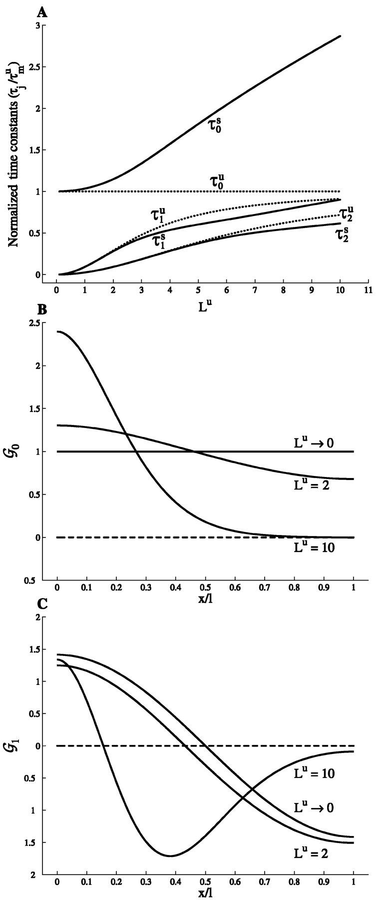
Time constants and eigenfunctions. A, The system time constant τ₀ and the first two equalizing time constants, τ₁ and τ₂, are normalized to the membrane time constant τ_m^u and plotted for a cylinder with sealed ends, as a function of the electrotonic length L^u(L^u ≤ 10). Both the uniform case (dotted lines) and the maximal slope case (solid lines) are shown. Explicit analytical solutions are available in the uniform case. The values in the slope case were computed by solving a transcendental equation as explained in Appendix E. B, Eigenfunction 𝒢₀^s as a function of the dimensionless variable y = x/ℓ in the maximal slope case for two values of L^u (2 and 10) and in the limit L^u → 0 (where the uniform case is recovered). 𝒢₀^s(y) was computed as explained in Appendix E. C, Same for the eigenfunction 𝒢₁^s(y). The convention that 𝒢_j^s(0) > 0 was adopted. The reader is referred to Appendix D.1 for further elaborations.

The equalizing time constants τ_j, j > 1, all vanish with L^u as (L^u)², as in the uniform case (see Appendix E). However, at variance with τ₀^s, they are smaller in the maximal slope case than in the uniform case for small L^u values, as proved in Appendix E.2. This is in contrast with their behavior at large L^u, where they are larger than in the uniform case and go to infinity with L^u(see Appendix E.2). For instance, τ₁^s is smaller than τ₁^u as long as L^u< 10, and then becomes larger than τ₁^u, as can be seen in Figure 9A. Note also that τ_j^ssignificantly departs from τ_j^u only for large enough L^u (typically L^u > jπ). This means that, at variance with τ₀, the time course of voltage equalization is little affected by the conductance gradient for physiologically reasonable values of L^u. In this range, differences with respect to the uniform case occur only for the first equalizing time constants and only for rather large values of L^u(L^u > 3) and do not exceed 20%.

As in the uniform case, the eigenfunctions oscillate faster and faster as j increases, the function 𝒢_j vanishing exactly j times on the open interval (0, ℓ). This is illustrated in Figures 9B, C, where the first two modes, 𝒢₀^s(y) and 𝒢₁^s(y), are plotted for the maximal slope case and sealed end boundary conditions. At variance with the uniform case, they are not pure Fourier modes: they show some degree of spatial localization, their amplitude being larger in the low conductance region of the cable (Fig. 9B, C). In particular, 𝒢₀^s(x) is not a constant. For sealed end boundary conditions, it is a monotonic function of x, as proved in Appendix E, reaching its maximum at the proximal end (x = 0), where the membrane conductance is minimal, whereas its minimum is obtained at the distal end (x = ℓ) where the membrane conductance is maximal. This means that in the final stage of voltage relaxation when the voltage decays everywhere at the same rate τ₀^s, the cable is not isopotential, at variance with the uniform case. At this time, axial current constantly flows from the low membrane conductance region to the high conductance region, maintaining a voltage gradient. The nonuniformity of 𝒢₀^s increases with L^u. It disappears when L^u goes to 0; the uniform solution 𝒢₀^u(y) = 1 is then recovered. For large values of L^u(L^u = 10), 𝒢₀^s(y) develops an exponentially decreasing tail in the high conductance region (this feature is discussed in Appendix D.1). Slow voltage transients will then be observed only in the low conductance region during the final relaxation phase. We note that current injection in the high conductance region will lead to small voltage transients. The other eigenfunctions display a similar behavior as 𝒢₀(y) , as illustrated in Figure 9C in the case of 𝒢₁^s(y) . As previously noticed for τ_j^s, compared with 𝒢₀^s(y) , larger values of L^u are required to observe strong departures of 𝒢₁^s(y) from the cosine profiles of the uniform case. This supports the general conclusion that for values of L^u typical of dendrites (L^u = 1 − 3), conductance gradients affect the slow asymptotic relaxation of the potential but have little effect on the faster “equalization” process. Note also that steeper conductance profiles lead to a slower relaxation and a stronger localization of 𝒢₀ (result not shown).

DISCUSSION

Main results and insights

The first general conclusion drawn from this work is that for cylindrical cables with both ends sealed, monotonic increase in G_m increases the transfer resistance from any input location to the proximal end (soma) compared with the corresponding uniform case. Thus, an increasing G_m(x) results in an increase of the voltage response at the soma. This effect is more pronounced when the steepness of G_m(x) increases. Importantly, this improvement, caused by monotonic increase in G_m, is also generally valid in reconstructed passive dendritic trees, although exceptions are expected for relatively long distal dendritic arbors. When synaptic inputs (rather than current inputs) are involved, the advantage of membrane nonuniformity becomes even more pronounced (double “benefit”) for distal synaptic inputs. This is caused by the larger leakiness of the membrane at distal dendritic sites in the nonuniform case, which results in a decrease in the local synaptic saturation, and thus, with the generation of more current by these distal synapses [see alsoBernander et al. (1994)].

The second general result is that any membrane nonuniformity decreases the electrotonic length (L) of the cable, compared with the corresponding uniform case. However, this increase in the cable “compactness” in nonuniform cylinders does not necessarily imply an increase in voltage (or charge) transfer because L is not the sole parameter of importance in this case. Indeed, for (both geometrically and electrically) nonuniform cylinders, voltage attenuation also depends on the direction of current flow. For example, in cylinders with both ends sealed and with a monotonic increase in membrane conductance, the attenuation of voltage from the leaky end to the other end is smaller than in the reverse direction.

Another general result, which holds true for all cable structures with sealed ends (as neurons typically are), is that any membrane heterogeneity slows the final relaxation of voltage as compared with the corresponding uniform case. In other words, for any nonuniformity, the slowest time constant, τ₀, is always larger than τ_m^u, the slowest time constant in the corresponding uniform case. Thus, the final decay (the “tail”) of the excitatory synaptic potentials (e.g., the somatic EPSPs) is expected to be slower when the dendritic membrane conductance is spatially nonuniform, and this effect increases with L. The slowing down of the final decay attributable to membrane nonuniformity has important implications for synaptic integration and for the experimental estimation of L (see below).

A general insight from studying the transient signals is that the system time constant τ₀ is a global quantity (i.e., it is the same everywhere, even in an heterogeneous cable). This results from the spatial averaging that takes place in the dendritic tree. Consequently, the properties of local electrical signals in dendrites are shaped, to a large extent, by the passive characteristics of the dendritic tree. Even an active local signal is strongly affected by the passive properties of the not-yet-activated adjacent regions. Thus, one cannot fully understand active phenomena in neurons without understanding the interplay between the underlying passive and active mechanisms.

Finally, we have shown that in cable structures with membrane nonuniformity and both ends sealed, there is a voltage gradient (an axial current) when the voltage relaxes according to τ₀, whereas in the uniform case, the whole structure is isopotential at this time. In the former case, the voltage is larger at sites with less leaky membrane conductance (namely, axial current constantly flows from these sites to the leakier regions). The experimental implication of this result is highlighted below.

Implications for experiments: estimating L and assessing membrane nonuniformity

The theoretical results presented in this work have two direct implications from the experimental viewpoint. The first concerns the estimation of the electrotonic length, L, of the dendritic tree. One of the most powerful experimental outcomes of Rall’s cable theory for dendrites was his “peeling” method for estimating L from the two slowest time constants (τ₀ and τ₁), which were “peeled” from experimental transients (Rall, 1969). Rall has analytically shown that, in uniform passive cylinders with both ends sealed:

$$L=\frac{\pi }{\sqrt{{\tau }_0/{\tau }_1-1}}.$$ Equation 7

What happens when this equation is used with the first two time constants estimated by peeling transients in the nonuniform case, namely, when τ₀^s and τ₁^s (in the slope case for example) are used in the above equation? We have shown above that τ₀^s is larger than τ_m^uand that, for relatively short cables, τ₁^s is smaller than τ₁^u. Therefore, one expects that the estimated L value, L_peel^s, in the slope case will be smaller than L^u in the corresponding uniform case.

This is indeed the case as shown in Figure10 where the L value estimated from peeling transients in the uniform case is compared with the estimate obtained when voltage transients of the slope case are peeled. In the uniform case, the L value estimated from peeling is very close to the actual value of L^u for the full range of L^u value tested (45° line, ⋄). In the slope case, however, this estimate saturates for cylinder with L^u > 2 (○). Namely, for L^u > 2, L^s_peel underestimates L^u. One could rightly argue that the estimate should be compared with the generalized electrotonic length (L = ∫₀^ℓ dx/λ(x)) rather than with L^u. Yet, the generalized electrotonic length is not expected to saturate (Fig. 10, •) as does L_peel^s. We thus conclude that when the peeling method is used in cases with monotonic increase in G_m, the value obtained for L may severely underestimate both the value of L in the corresponding uniform case (L^u) as well as the value of the generalized electrotonic length of the structure. We note that because τ₀^s and τ₁^s are independent of input location, the estimated L value is, generally, also independent of the location of current input (and voltage recording).

Fig. 10.

Errors in estimating L in the slope case. The electrotonic length of the cylinders was estimated usingRall’s (1969) peeling method (Eq. 7). The values of the first two time constants, τ₀ and τ₁, were peeled from a voltage response to a short current pulse injected to the compartmental model of the corresponding cylinder. The estimate is accurate for uniform cylinders (⋄), but in the slope case (○), both L^u and the generalized electrotonic lengths (●) are underestimated for cylinders with L^u > 2.

Another theoretical prediction that has a direct experimental relevance is the “crossing,” in the nonuniform case, of voltage transients measured simultaneously at distal and proximal locations (Fig. 8,right traces, top). As discussed above, in nonuniform cables there is a constant current flow from low-conductance regions to high-conductance regions when the voltage transient relaxes with τ₀. In the nonuniform case, when the input is delivered to distal leaky regions, the resultant voltage is initially larger near the input site, but at later times it becomes larger at proximal, less leaky sites. This implies a crossing of the voltage transients measured proximally and distally in the nonuniform case but not in the corresponding uniform case (where the structure is isopotential at large times), as indeed shown in Figure 8 (right traces). Crossing of transients may take place also in the uniform case in the experimentally less likely situation where one electrode is near a sealed end boundary. At this location, charge tends to accumulate, and voltage transients relax slower than in more proximal locations. This may yield voltage crossing between faster decaying proximal transients and voltage transients measured near this boundary.

In conclusion, when voltage transients recorded at two dendritic locations cross each other, this strongly suggests that the membrane conductance is not uniformly distributed over the dendrites. Such a “cross-over” was indeed recently described in the experiments ofStuart and Spruston (1998) [see also “crossing” in Rapp et al. (1994), their Fig. 8].

Implications on membrane nonuniformity for the input–output function of neurons

This work analyzes the flow of current from the dendrites to the soma, showing that transfer impedance to the soma increases when relatively fewer ion channels are allocated near the soma and more are allocated distally. This gradient of ion channels also implies that the dendritic tree imposes a smaller load (current sink) on the spike mechanism in the axon compared with the corresponding uniform case. This is demonstrated in Figure 11 where the I/f curves of a modeled neuron with uniform (dotted curve) versus slope (continuous line) dendritic membrane conductance are shown. In both cases, the same excitable axon is attached to the soma. As can be seen, relatively less current is required to reach threshold for action potential firing in the slope case, and the I/f in this case is somewhat more linear (at low firing rates) than in the corresponding uniform case. Thus, a smaller number of excitatory synapses are required to fire the axon when the dendrites have a slope conductance.

Fig. 11.

The conductance profile, G_m(x), in the dendrites affects the I/f relation of the neuron. An excitable axon (Mainen and Sejnowski, 1996) was added to the passive dendritic model of layer V pyramid shown in Figure 7B. Constant current I was injected to the soma in both the uniform case (dotted line) and the slope case (continuous line). In the later case the dendritic tree imposes a smaller “current sink” on the firing mechanism at the axon. Consequently, the I/f curve is shifted to the left. The bottom traceshows the action potentials in the uniform case (dotted line) and the slope case (continuous line) on a 100 msec time interval for I = 0.25 nA.

One may wonder why the dendritic membrane should possess ion channels at all. One could argue that signal transfer would be most efficient when the dendritic tree is essentially bare of ion channels (no current loss via the dendritic membrane). However, this would imply that the membrane time constant is very large, and consequently, that the resetting of the dendritic voltage is very slow. Another undesirable consequence of very low membrane conductance is that each synaptic input (conductance change) will dramatically change the effective membrane time constant and input resistance. Leaky resting membrane ensures that the effective (integration) time constant and the input resistance remain within a reasonable value even when a massive synaptic input bombards the neuron (Bernander et al., 1991; Rapp et al., 1992). Redistribution of approximately the same number of ion channels in the dendritic tree enables one to modulate signal processing in the dendritic tree, still ensuring that both the temporal characteristics of the signal and its amplitude will remain within a desired operating regime.

The present study explored the most straightforward case in which the total number of ion channels within the modeled structure remains fixed. There is, of course, the possibility that the number (and type) of effective dendritic ion channels change both very rapidly (e.g., because of the activation of synaptic-gated conductances as well as of voltage-gated ion currents with fast kinetics such as I_A) or at a slower time scale where the production of new ion channels is involved. Whatever the mechanism is, it is clear that because of its membrane ion channels, the dendritic tree becomes a very flexible electrical device that can dynamically modulate, at different time scales its input–output capabilities.

REFERENCES

- 1.Abbott LF. Simple diagrammatic rules for solving dendritic cable problems. Physica A. 1992;185:343–356. [Google Scholar]
- 2.Abbott LF, Farhi E, Gutmann S. The path integral for dendritic trees. Biol Cybern. 1991;66:49–60. doi: 10.1007/BF00196452. [DOI] [PubMed] [Google Scholar]
- 3.Abramowitz M, Stegun IA. Handbook of mathematical functions. Dover; New York: 1970. [Google Scholar]
- 4.Agmon-Snir H, Segev I. Signal delay and input synchronization in passive dendritic structures. J Neurophysiol. 1993;70:2066–2085. doi: 10.1152/jn.1993.70.5.2066. [DOI] [PubMed] [Google Scholar]
- 5.Barrett JN, Crill WE. Specific membrane properties of cat motoneurones. J Physiol (Lond) 1974;239:301–324. doi: 10.1113/jphysiol.1974.sp010570. [DOI] [PMC free article] [PubMed] [Google Scholar]
- 6.Bernander O, Douglas RJ, Martin KA, Koch C. Synaptic background activity determines spatio-temporal integration in single pyramidal cells. Proc Natl Acad Sci USA. 1991;88:11569–11573. doi: 10.1073/pnas.88.24.11569. [DOI] [PMC free article] [PubMed] [Google Scholar]
- 7.Bernander O, Koch C, Douglas RJ. Amplification and linearization of distal synaptic input to cortical pyramidal cells. J Neurophysiol. 1994;72:2743–2753. doi: 10.1152/jn.1994.72.6.2743. [DOI] [PubMed] [Google Scholar]
- 8.Bischofberger J, Jonas P. Action potential propagation into the presynaptic dendrites of rat mitral cells. J Physiol (Lond) 1997;504:359–365. doi: 10.1111/j.1469-7793.1997.359be.x. [DOI] [PMC free article] [PubMed] [Google Scholar]
- 9.Bressloff PC, Taylor JG. Compartmental-model response function for dendritic trees. Biol Cybern. 1993;70:199–207. [Google Scholar]
- 10.Butz EG, Cowan JD. Transient potentials in dendritic systems of arbitrary geometry. Biophys J. 1974;14:661–689. doi: 10.1016/S0006-3495(74)85943-6. [DOI] [PMC free article] [PubMed] [Google Scholar]
- 11.Chen WR, Midtgaard J, Shepherd GM. Forward and backward propagation of dendritic impulses and their synaptic control in mitral cells. Science. 1997;278:463–467. doi: 10.1126/science.278.5337.463. [DOI] [PubMed] [Google Scholar]
- 12.Clements JD, Redman SJ. Cable properties of cat spinal motoneurones measured by combining voltage clamp, current clamp and intracellular staining. J Physiol (Lond) 1989;409:63–87. doi: 10.1113/jphysiol.1989.sp017485. [DOI] [PMC free article] [PubMed] [Google Scholar]
- 13.De Schutter E, Bower JM. Simulated responses of cerebellar Purkinje cells are independent of the dendritic location of granule cell synaptic inputs. Proc Natl Acad Sci USA. 1994;91:4736–4740. doi: 10.1073/pnas.91.11.4736. [DOI] [PMC free article] [PubMed] [Google Scholar]
- 14.Dodt HU, Zieglgansberger W. Infrared videomicroscopy: a new look at neuronal structure and function. Trends Neurosci. 1994;17:453–458. doi: 10.1016/0166-2236(94)90130-9. [DOI] [PubMed] [Google Scholar]
- 15.Durand D. The somatic shunt cable model for neurons. Biophys J. 1984;46:645–653. doi: 10.1016/S0006-3495(84)84063-1. [DOI] [PMC free article] [PubMed] [Google Scholar]
- 16.Fleshman JW, Segev I, Burke RE. Electrotonic architecture of type-identified α-motoneurons in the cat spinal cord. J Neurophysiol. 1988;60:60–85. doi: 10.1152/jn.1988.60.1.60. [DOI] [PubMed] [Google Scholar]
- 17.Haag J, Borst A. Amplification of high-frequency synaptic inputs by active dendritic membrane processes. Nature. 1996;379:639–641. [Google Scholar]
- 18.Hille B. Ionic channels of excitable membranes. Sinauer; Sunderland, MA: 1992. [Google Scholar]
- 19.Hines ML, Carnevale NT. The NEURON simulation environment. Neural Comput. 1997;9:1179–1209. doi: 10.1162/neco.1997.9.6.1179. [DOI] [PubMed] [Google Scholar]
- 20.Hoffman DA, Magee JC, Colbert CM, Johnston D. K+ channels regulation of signal propagation in dendrites of hippocampal pyramidal neurons. Nature. 1997;387:869–875. doi: 10.1038/43119. [DOI] [PubMed] [Google Scholar]
- 21.Holmes WR. The role of dendritic diameters in maximizing the effectiveness of synaptic inputs. Brain Res. 1989;478:127–137. doi: 10.1016/0006-8993(89)91484-4. [DOI] [PubMed] [Google Scholar]
- 22.Holmes WR, Rall W. Electrotonic length estimates in neurons with dendritic tapering or somatic shunt. J Neurophysiol. 1992a;68:1421–1437. doi: 10.1152/jn.1992.68.4.1421. [DOI] [PubMed] [Google Scholar]
- 23.Holmes WR, Rall W. Estimating the electrotonic structure of neurons with compartmental models. J Neurophysiol. 1992b;68:1438–1451. doi: 10.1152/jn.1992.68.4.1438. [DOI] [PubMed] [Google Scholar]
- 24.Holmes WR, Segev I, Rall W. Interpretation of time constant and electrotonic length estimates in multicylinder or branched neuronal structures. J Neurophysiol. 1992;68:1401–1420. doi: 10.1152/jn.1992.68.4.1401. [DOI] [PubMed] [Google Scholar]
- 25.Holmes WR, Woody CD. Effects of uniform and non-uniform synaptic “activation-distributions” on cable properties of modeled cortical pyramidal neurons. Brain Res. 1989;505:12–22. doi: 10.1016/0006-8993(89)90110-8. [DOI] [PubMed] [Google Scholar]
- 26.Horwitz B. An analytical method for investigating transient potentials in neurons with branching dendritic trees. Biophys J. 1981;36:155–192. doi: 10.1016/S0006-3495(81)84722-4. [DOI] [PMC free article] [PubMed] [Google Scholar]
- 27.Horwitz B. Unequal diameters and their effects on time-varying voltages in branched neurons. Biophys J. 1983;41:51–66. doi: 10.1016/S0006-3495(83)84405-1. [DOI] [PMC free article] [PubMed] [Google Scholar]
- 28.Iansek R, Redman SJ. An analysis of the cable properties of spinal motoneurones using a brief intracellular current pulse. J Physiol (Lond) 1973;234:613–636. doi: 10.1113/jphysiol.1973.sp010364. [DOI] [PMC free article] [PubMed] [Google Scholar]
- 29.Johnston D, Magee JC, Colbert CM, Cristie BR. Active properties of neuronal dendrites. Annu Rev Neurosci. 1996;19:165–186. doi: 10.1146/annurev.ne.19.030196.001121. [DOI] [PubMed] [Google Scholar]
- 30.Kavalali E, Zhuo M, Bito H, Tsien R. Dendritic Ca2+ channels characterized by recordings from isolated hippocampal dendritic segments. Neuron. 1997;18:651–663. doi: 10.1016/s0896-6273(00)80305-0. [DOI] [PubMed] [Google Scholar]
- 31.Kawato M. Cable properties of a neuron model with nonuniform membrane resistivity. J Theor Biol. 1984;111:149–169. doi: 10.1016/s0022-5193(84)80202-7. [DOI] [PubMed] [Google Scholar]
- 32.Koch C. Biophysics of Computation: information processing in single neurons. Oxford UP; Oxford: 1999. [Google Scholar]
- 33.Landau LD, Lifschitz EM. Quantum mechanics, Ed 3. Butterworth-Heinemann; Oxford: 1997. [Google Scholar]
- 34.Laurent G, Seymour-Laurent KJ, Johnson K. Dendritic excitability and a voltage-gated calcium current in locust nonspiking local interneurons. J Neurophysiol. 1993;69:1484–1498. doi: 10.1152/jn.1993.69.5.1484. [DOI] [PubMed] [Google Scholar]
- 35.Llinas R, Sugimori M. Electrophysiological properties of in vitro Purkinje cell dendrites in mammalian cerebellar slices. J Physiol (Lond) 1980;305:197–213. doi: 10.1113/jphysiol.1980.sp013358. [DOI] [PMC free article] [PubMed] [Google Scholar]
- 36.Lorente de No’ R. Action potential of the motoneurons of the hypoglossus nucleus. J Cell Comp Physiol. 1947;29:207–287. doi: 10.1002/jcp.1030290303. [DOI] [PubMed] [Google Scholar]
- 37.Magee JC. Dendritic hyperpolarization-activated currents modify the integrative properties of hippocampal CA1 pyramidal neurons. J Neurosci. 1998;18:7613–7624. doi: 10.1523/JNEUROSCI.18-19-07613.1998. [DOI] [PMC free article] [PubMed] [Google Scholar]
- 38.Mainen ZF, Sejnowski TJ. Influence of dendritic structure on firing pattern in model neocortical neurons. Nature. 1996;382:363–366. doi: 10.1038/382363a0. [DOI] [PubMed] [Google Scholar]
- 39.Major G, Evans JD, Jack JJB. Solutions for transients in arbitrarily branching cables: I. Voltage recording with a somatic shunt. Biophys J. 1993a;65:423–449. doi: 10.1016/S0006-3495(93)81037-3. [DOI] [PMC free article] [PubMed] [Google Scholar]
- 40.Major G, Evans JD, Jack JJB. Solutions for transients in arbitrarily branching cables: II. Voltage clamp theory. Biophys J. 1993b;65:450–468. doi: 10.1016/S0006-3495(93)81038-5. [DOI] [PMC free article] [PubMed] [Google Scholar]
- 41.Major G, Evans JD, Jack JJB. Solutions for transients in arbitrarily branching cables: III. Voltage clamp problems. Biophys J. 1993c;65:469–491. doi: 10.1016/S0006-3495(93)81039-7. [DOI] [PMC free article] [PubMed] [Google Scholar]
- 42.Mel BW. Information processing in dendritic trees. Neural Comput. 1994;6:1427–1439. [Google Scholar]
- 43.Miller JP, Rall W, Rinzel J. Synaptic amplification by active membrane in dendritic spines. Brain Res. 1985;325:325–330. doi: 10.1016/0006-8993(85)90333-6. [DOI] [PubMed] [Google Scholar]
- 44.Nicoll A, Larkman A, Blakemore C. Modulation of EPSP shape and efficacy by intrinsic membrane conductances in rat neocortical pyramidal neurons in vitro. J Physiol (Lond) 1993;468:693–710. doi: 10.1113/jphysiol.1993.sp019795. [DOI] [PMC free article] [PubMed] [Google Scholar]
- 45.Pinsky PF, Rinzel J. Intrinsic and network rhythmogenesis in a reduced traub model for CA3 neurons. J Comput Neurosci. 1994;1:39–60. doi: 10.1007/BF00962717. [DOI] [PubMed] [Google Scholar]
- 46.Poznanski RR. Membrane voltage changes in passive dendritic trees: a tapering equivalent cylinder model. IMA J Math Appl Med Biol. 1988;5:113–145. doi: 10.1093/imammb/5.2.113. [DOI] [PubMed] [Google Scholar]
- 47.Rall W. Branching dendritic trees and motoneuron membrane resistivity. Exp Neurol. 1959;1:491–527. doi: 10.1016/0014-4886(59)90046-9. [DOI] [PubMed] [Google Scholar]
- 48.Rall W. Theory of physiological properties of dendrites. Ann NY Acad Sci. 1962;96:1071–1092. doi: 10.1111/j.1749-6632.1962.tb54120.x. [DOI] [PubMed] [Google Scholar]
- 49.Rall W. Time constants and electrotonic length of membrane cylinders and neurons. Biophys J. 1969;9:1483–1508. doi: 10.1016/S0006-3495(69)86467-2. [DOI] [PMC free article] [PubMed] [Google Scholar]
- 50.Rall W, Agmon-Snir H. Cable theory for dendritic neurons. In: Koch C, Segev I, editors. Methods in neuronal modeling: from ions to networks, Ed 2. MIT; Cambridge, MA: 1998. pp. 27–92. [Google Scholar]
- 51.Rall W, Rinzel J. Branch input resistance and steady attenuation for input to one branch of a dendritic neuron model. Biophys J. 1973;13:648–688. doi: 10.1016/S0006-3495(73)86014-X. [DOI] [PMC free article] [PubMed] [Google Scholar]
- 52.Rall W, Shepherd GM. Theoretical reconstruction of field potentials and dendrodendritic synaptic interactions in olfactory bulb. J Neurophysiol. 1968;31:884–915. doi: 10.1152/jn.1968.31.6.884. [DOI] [PubMed] [Google Scholar]
- 53.Rapp M, Segev I, Yarom Y. Physiology, morphology and detailed passive models of cerebellar Purkinje cells. J Physiol (Lond) 1994;474:101–118. doi: 10.1113/jphysiol.1994.sp020006. [DOI] [PMC free article] [PubMed] [Google Scholar]
- 54.Rapp M, Yarom Y, Segev I. The impact of parallel fiber background activity on the cable properties of cerebellar Purkinje cells. Neural Comput. 1992;4:518–533. [Google Scholar]
- 55.Rinzel J, Rall W. Transient response in a dendritic neuron model for current injected at one branch. Biophys J. 1974;14:759–790. doi: 10.1016/S0006-3495(74)85948-5. [DOI] [PMC free article] [PubMed] [Google Scholar]
- 56.Schierwagen AK. A non-uniform equivalent cable model of membrane voltage changes in a passive dendritic tree. J Theor Biol. 1989;141:159–179. doi: 10.1016/s0022-5193(89)80015-3. [DOI] [PubMed] [Google Scholar]
- 57.Schwindt PC, Crill WE. Amplification of synaptic current by persistent sodium conductance in apical dendrite of neocortical neurons. J Neurophysiol. 1995;74:2220–2224. doi: 10.1152/jn.1995.74.5.2220. [DOI] [PubMed] [Google Scholar]
- 58.Segev I, Friedman A, White E, Gutnick M. Electrical consequences of spine dimensions in a model of a cortical spiny stellate cell completely reconstructed from serial thin sections. J Comput Neurosci. 1995;2:117–130. doi: 10.1007/BF00961883. [DOI] [PubMed] [Google Scholar]
- 59.Segev I, Rall W. Computational study of an excitable dendritic spine. J Neurophysiol. 1988;60:499–523. doi: 10.1152/jn.1988.60.2.499. [DOI] [PubMed] [Google Scholar]
- 60.Segev I, Rall W. Excitable dendrites and spines: earlier theoretical insights elucidate recent direct observations. Trends Neurosci. 1998;21:453–460. doi: 10.1016/s0166-2236(98)01327-7. [DOI] [PubMed] [Google Scholar]
- 61.Shepherd GM, Brayton RK, Miller JP, Segev I, Rinzel J, Rall W. Signal enhancement in distal cortical dendrites by means of interactions between active dendritic spines. Proc Natl Acad Sci USA. 1985;82:2192–2195. doi: 10.1073/pnas.82.7.2192. [DOI] [PMC free article] [PubMed] [Google Scholar]
- 62.Siegel M, Marder E, Abbott LF. Activity-dependent current distributions in model neurons. Proc Natl Acad Sci USA. 1994;91:11308–11312. doi: 10.1073/pnas.91.24.11308. [DOI] [PMC free article] [PubMed] [Google Scholar]
- 63.Spencer WA, Kandel ER. Electrophysiology of hippocampal neurons. IV. Fast pre-potentials. J Neurophysiol. 1961;24:272–285. doi: 10.1152/jn.1961.24.3.272. [DOI] [PubMed] [Google Scholar]
- 64.Spiegel MR. Mathematical handbook. Schaum’s outline series. McGraw-Hill; New York: 1968. [Google Scholar]
- 65.Stuart G, Häusser M. Initiation and spread of sodium action potentials in cerebellar Purkinje cells. Neuron. 1994;13:703–712. doi: 10.1016/0896-6273(94)90037-x. [DOI] [PubMed] [Google Scholar]
- 66.Stuart GM, Dodt HU, Sakmann B. Patch-clamp recordings from the soma and dendrites of neurons in brain slices using infrared video microscopy. Pflügers Arch. 1993;423:511–518. doi: 10.1007/BF00374949. [DOI] [PubMed] [Google Scholar]
- 67.Stuart GM, Sakmann B. Amplification of EPSPs by axosomatic sodium channels in neocortical pyramidal neurons. Neuron. 1995;15:1–20. doi: 10.1016/0896-6273(95)90095-0. [DOI] [PubMed] [Google Scholar]
- 68.Stuart GM, Spruston N. Determinants of voltage attenuation in neocortical pyramidal neuron dendrites. J Neurosci. 1998;18:3501–3510. doi: 10.1523/JNEUROSCI.18-10-03501.1998. [DOI] [PMC free article] [PubMed] [Google Scholar]
- 69.Turrigiano G, LeMasson G, Marder E. Selective regulation of current densities underlies spontaneous changes in the activity of cultured neurons. J Neurosci. 1995;15:3640–3652. doi: 10.1523/JNEUROSCI.15-05-03640.1995. [DOI] [PMC free article] [PubMed] [Google Scholar]
- 70.Wilson CJ. Dynamic modification of dendritic cable properties and synaptic transmission by voltage-gated potassium channels. J Comput Neurosci. 1995;2:91–115. doi: 10.1007/BF00961882. [DOI] [PubMed] [Google Scholar]
- 71.Wolfram S. Mathematica: a System for doing mathematics by computer, Ed 2. Addison-Wesley; Redding, MA: 1991. [Google Scholar]