The Magnitude and Phase of Temporal Modulation Transfer Functions in Cat Auditory Cortex

Abstract

Temporal modulation transfer functions (tMTFs) in response to periodic click trains are presented for simultaneous recordings from primary auditory cortex, anterior auditory field, and secondary auditory cortex in 21 cats. The multiunit records could be separated in to 215 single-unit spike trains that allowed a reliable estimate of a group delay, which represents the cumulative delay for responses to repetitive stimuli. For approximately two-thirds of the 215 single units the group delay was within 7.5 msec of the response latency to the first clicks in the trains. For the remaining units, the group delay was on average ∼14 msec higher, and this may result from differences in synaptic properties. These findings were similar in the three cortical areas studied. The findings are modeled based on presynaptic facilitation and depression and pyramidal cell calcium kinetics, and a quantitative description of the magnitude of the tMTF was obtained that resulted in substantially shorter depression time constants (20 msec) than reported for visual cortex (300 msec). A small amount (0–5.5%) of facilitation that decayed with a time constant of 60 msec was obtained. Auditory cortical cells apparently have much faster recovery mechanisms than visual cortical cells. This allows for the ability of the auditory cortex to reliably track the rhythms that occur in natural sounds.

Communication sounds have both spectral and temporal aspects. The timing aspects are evident in the onset and offset and in the amplitude and frequency modulation of the sound. In humans, amplitude-modulated (AM) tones or AM noise produce various hearing sensations depending on the modulation frequency. These include rhythm and fluctuation strength for AM frequencies below ∼20 Hz and roughness and pitch for AM frequencies above 20 Hz (Zwicker and Fastl, 1990). The ability of neurons to code the AM aspects of sound in a temporal manner is represented by the temporal modulation transfer function (tMTF; Schreiner and Langner, 1988). For a fixed modulation depth of the AM stimuli, the tMTF is equal to the Fourier transform of the period histograms of the neuronal firings. Generally, only the magnitude of the Fourier component with a modulation frequency (MF) corresponding to the period duration of the AM is considered.

Because the Fourier transform is complex, the tMTF is a complex function and is characterized by its magnitude as well as its phase dependence on MF. The phase–MF dependence allows calculation of the group delay at each MF by taking the local slope of the phase–MF function (Papoulis, 1977). The group delay is a measure over a group of frequencies. In case the phase–MF function for most of the MF range can be approximated by a straight line, the group delay is independent of the MF over that range, represents a pure delay, and can be interpreted as a neuron property (Anderson et al., 1971).

By using 1-sec-duration periodic click trains as the AM stimulus followed by 2 sec of silence (Eggermont, 1991), one can independently estimate the latency of the unadapted response to the first click in each train. The difference between the group delay, which represents the cumulative delay for responses to repetitive stimuli, and the latency of the response to first clicks in the trains can be interpreted as the result of temporal filtering. This allows an estimate of the contribution of this temporal filtering process to the group delay. The temporal filtering is likely the result of presynaptic mechanisms such as facilitation and depression (Varela et al., 1997) and postsynaptic mechanisms such as afterhyperpolarization and Ca²⁺ dynamics (Wang, 1998). Facilitation and depression are presumed to be multiplicative and to have exponential time courses (Magleby, 1987; Varela et al., 1997). For neocortical synapses, depression appears to be more pronounced than facilitation (Markram et al., 1998).

In this paper, the complex tMTFs in response to periodic click trains are analyzed, and a model based on presynaptic facilitation and depression and pyramidal cell calcium kinetics is presented that provides a quantitative description of the magnitude of the tMTF. The results suggest that recovery time constants are much shorter in auditory cortex than in visual cortex.

MATERIALS AND METHODS

The care and the use of animals reported on in this study was in accordance with the Guide to the Care and Use of Experimental Animals and was approved (P88095) by the Life and Environmental Sciences Animal Care Committee of the University of Calgary.

Animal preparation. Cats were premedicated with 0.25 ml/kg body weight of a mixture of 0.1 ml of acepromazine (0.25 mg/ml) and 0.9 ml of atropine methyl nitrate (5 mg/ml) subcutaneously. After ∼0.5 hr they received an intramuscular injection of 25 mg/kg ketamine (100 mg/ml) and 20 mg/kg pentobarbital sodium (65 mg/ml). Lidocaine (20 mg/ml) was injected subcutaneously and rubbed in gently, and then a skin flap was removed and the skull cleared from overlying muscle tissue. A large screw was cemented upside-down on the skull with dental acrylic. An 8-mm-diameter hole was trephined over the right temporal cortex to expose parts of primary auditory cortex (AI) and secondary auditory cortex (AII). A 4 mm hole was drilled over the anterior auditory field (AAF). The dura was left intact, and the brain was covered with light mineral oil. Then the cat was placed in a sound-treated room on a vibration isolation frame, and the head was secured with the screw. Additional acepromazine-atropine mixture was administered every 2 hr. Light anesthesia was maintained with intramuscular injections of ketamine at dosages of 2–5 mg · kg⁻¹ · hr⁻¹. The wound margins were infused every 2 hr with lidocaine and, also every 2 hr new mineral oil was added if needed. The temperature of the cat was maintained at 37°C. At the end of the experiment the animals were killed with an overdose of pentobarbital sodium.

Acoustic stimulus presentation. Acoustic stimuli were presented in an anechoic room from a speaker placed 55 cm in front of the cat’s head. The sound-treated room was made anechoic for frequencies >625 Hz by covering walls and ceiling with acoustic wedges (3 inch; SONEX, Minneapolis, MN) and by covering exposed parts of the vibration isolation frame, equipment, and floor with wedge material as well. Calibration and monitoring of the sound field were done using a Brüel & Kjær (Atlanta, GA) type 4134 microphone placed above the animal’s head and facing the loudspeaker. A search stimulus consisting of random frequency tone pips, noise burst, and clicks was used to locate units. Characteristic frequency (CF) and tuning curve of the individual neurons were determined with a 50-msec-duration γ shape envelope, tone pips presented randomly in frequency once per second (Eggermont, 1996). After the frequency tuning properties of the cells at each electrode were determined, periodic click trains (1 sec duration followed by 2 sec of silence) were presented once per 3 sec. The click repetition rates were between 1 and 32 at logarithmically equal distance with four values per octave and were randomly presented. The sequences of 21 click trains were repeated 10 times, resulting in a total stimulus ensemble duration of 630 sec. The click trains were presented at peak intensities of 35, 55, and 75 dB sound pressure level (SPL), and results are presented for the intensity which resulted in the highest firing rate.

Recording and spike separation procedure. Three tungsten microelectrodes (Micro Probe Inc.) with impedances between 1.5 and 2.5mΩ were independently advanced perpendicular to the AI, AAF, and AII surfaces using remotely controlled, motorized hydraulic microdrives (Trent-Wells Mark III). The electrode signals were amplified using extracellular preamplifiers (2400; Dagan Instruments, Minneapolis, MN) and filtered between 200 Hz (VBF8; Kemo Ltd., Beckenham, UK; high-pass, 24 dB/octave) and 3 kHz (6 dB/octave, Dagan rolloff) to remove local field potentials. The signals were sampled through 12 bit analog-to-digital converters (DT 2752; Data Translation, Marlborough, MA) into a PDP 11/53 microcomputer, together with timing signals from three Schmitt triggers. In general the recorded signal on each electrode contained activity of two to four neural units. The PDP was programmed to separate these multiunit spike trains into single-unit spike trains using a maximum variance algorithm (Eggermont, 1996). The spikes from well separated waveform classes, each assumed to represent a particular neuron, were stored and coded for display.

In addition, the electrode signals were bandpass-filtered between 10 and 100 Hz to obtain spike-free signals of ongoing local field potentials (LFPs). These signals were also passed through Schmitt triggers set at ∼2 SDs (i.e., at approximately −100 μV) below the mean value of the ongoing signal during silence. The “spikes” of these LFPs were processed in the same way as single-unit spike data. We have shown previously that these level crossings explain most of the temporal (Eggermont and Smith, 1995) and spectral (Eggermont, 1996) response properties of the single units recorded at the same electrode.

The boundary between AI and AAF was explored by taking a series of LFP and multiunit measures from caudal to rostral and assuring that there was a gradual increase in CF, which reversed in direction when advancing to the AAF. The AII was identified anatomically and electrophysiologically based on the broader tuning curves and different response patterns compared with those in the central and ventral parts of AI. Recordings in AII were generally made from the ventrorostral part. Recording electrode positions in the three cortical areas were chosen such that recordings with approximately similar best frequencies (within 0.5 octave) at 50–70 dB SPL were obtained. Recordings were made between 600 and 1200 μm below the cortex surface.

Data analysis. The temporal modulation transfer functions were obtained by Fourier transformation of the period histograms (Eggermont, 1991). Each modulation period was divided into 16 bins, and only recordings with at least five counts in the maximum bin per 10 stimulus presentations at a rate of 8 Hz were further analyzed. The tMTF was estimated from the amplitude of the first harmonic of the period histogram. The best modulating frequency (BMF) was defined as the click rate for which the tMTF was maximal. The limiting rate was defined as the highest click rate at which the response was 50% of that at the BMF. Phase (Φ)-click repetition rate (CRR) functions were approximated by straight lines using linear regression analysis. Only neurons with R² > 0.9 for the regression line calculation were included in the analysis. The slope was converted in a group delay τ = 1/360 Φ/CRR. If Φ is in degrees and CRR is in hertz, then τ is in seconds.

Group delay at a certain CRR is defined as the slope of the phase repetition rate function at that specific CRR. Typically one uses a group delay if a multifrequency component signal is passed through a frequency filter, because different frequency components may undergo different phase delays. This shows up in a nonlinear dependence between phase and frequency. Most of the phase change occurs around the peak of the filter response function. If the phase is linearly dependent on frequency over the entire frequency range of interest, then the system functions as a pure delay system for signals composed of frequencies within that range (Ruston and Bordogna, 1986).

The responses at CRRs <5/sec are generally small. Because always 10 trains were presented for each CRR, and the bin width was relative (1/16) to the period of the CRR, the phase definition was no problem for those CRRs. And as Figure 1 indicates, the response was always in the first or second bin. For the higher CRR (>18 Hz), the bin size was small (1–2 msec), and consequently the distribution was broad. However, the phase was generally defined within a few bins, and if not well defined the phase was not entered into the regression line calculation. The phase at CRRs of >18/sec had hardly any effect on the slope of the regression line. Again, taking Figure 1 as an example, deleting the phase entries >18 Hz has no effect on the slope of the regression line.

Fig. 1.

Magnitude and phase of the temporal modulation transfer function for periodic click train stimulation for a single unit from the anterior auditory field. The magnitude is expressed in the number of synchronized spikes per click train; the phase (position of the peak response in the period histogram relative to the period length) is expressed in radians. The data points are indicated byasterisks; for the magnitude function a cubic spline interpolation was used, whereas a linear regression line was calculated for the phase data. The slope of the phase click rate regression line can be converted in a group delay (in seconds) through division by 2π, resulting in 32.8 msec.

All statistical analyses were performed using Statview 4.5. Graphics and systems analysis were done with Matlab, Powerpoint, and Horizon software.

Perstimulatory adaptation and response to periodic click stimulation. Spike frequency adaptation in cortical, regular spiking, pyramidal cells has been described by a model largely based on Ca²⁺-gated K⁺ conductances and manifests itself in an exponential decreasing firing rate with time after onset of a current pulse (Wang, 1998). Such exponential decay is also seen in the firing rate of auditory nerve fibers during tone burst stimulation and has been modeled previously in terms of birth-and-death Markov processes (Eggermont, 1985; Gillespie, 1992). We summarize that model here with slight modifications, to allow application to cortical neurons in response to click trains of fixed duration but variable number of clicks. For a long tone burst, the normalized firing rate,R(t), as a function of time after onset,t, is assumed to decay exponentially:

$$R(t)=R_{SS}+(1-R_{SS})exp(-t/{\tau }_{\text{adap}}),$$ Equation 1

where R_ss is the normalized steady-state or fully adapted firing rate, the unadapted onset firing rate obtained after a sufficiently long silent period is normalized to 1, and τ_adap is the time constant of the exponential decay of the firing rate. In terms of the birth-and-death model, τ_adap was equal to the inverse of the sum of a birth and death rate, λ and μ, determining the availability of postsynaptic receptor sites. It was assumed that after transmitter release, free receptor sites (for cortical pyramidal cells this will likely be the AMPA receptors) were activated at a very fast rate and then converted at a rate λ into an inactive or occupied state and subsequently recovered to the free state with rate μ. This resulted in a fraction of inactive receptors of λ/(λ + μ) and a fraction of free receptors that determined the steady state R_ss = 1 − λ/(λ + μ) = μ/(λ + μ). The steady state was reached with a time constant τ_adap = (λ + μ)⁻¹. Alternative interpretations of the birth and death rate in terms of depletion and filling of the immediate release transmitter store in the presynaptic terminal are also plausible (Eggermont, 1985). For the adaptation in cortical cells, the interpretation of these two rates likely has to be different (e.g., incorporating postactivation suppression), but the formal description is assumed to remain the same.

Consider next a forward masking experiment with a masking tone burst long enough, usually of the order of 100 msec, to allow the neuron to reach the steady-state firing level R_ss and followed after a silent interval, Δt, by a test tone burst with equal intensity and frequency as the masker. The onset firing rate to the test tone burst, r_on(Δt), increases with the length of the silent interval after the masker, however, with a slower time course than that for the perstimulatory adaptation:

$$r_{\text{on}}(\mathrm{\Delta }t)=R_{SS}+(1-R_{SS})(1-exp(-\mathrm{\Delta }t/{\tau }_{\text{recov}})),$$ Equation 2

with τ_recov = (μ)⁻¹.R_ss, τ_recov, and τ_adap are interrelated because they depend only on λ and μ:

$$R_{SS}={\tau }_{\text{adap}}/{\tau }_{\text{recov}}.$$ Equation 3

In this model, the knowledge of the perstimulatory adaptation time constant, τ_adap, and the adapted steady-state firing level, R_ss, is sufficient to predict the recovery time constant in a forward masking experiment (Eggermont, 1985).

In case the masker has a short duration, D, the steady-state firing level, R_ss, has to be replaced by the appropriate adaptation level obtained for that duration. One obtains:

$$r_{\text{on}}(\mathrm{\Delta }t,D)=R_{\text{adap}}+(1-R_{\text{adap}})[1-exp(-\mathrm{\Delta }t/{\tau }_{\text{recov}})],$$ Equation 4A

$$=1-dexp(-\mathrm{\Delta }t/{\tau }_{\text{recov}}),$$ Equation 4B

with:

$$R_{\text{adap}}=R_{SS}[1-exp(-D/{\tau }_{\text{adap}})],$$ Equation 4C

d = (1 −R_adap) can be considered the fraction of depression produced by a single click.

For repetitive stimulation, generally with short-duration stimuli such as clicks, the cumulative effects of incomplete perstimulatory adaptation and incomplete recovery has to be taken into account. Under the assumption that the adaptation and recovery after the second click in a train are scaled versions of those after the first click, i.e., the adaptation starts from the level given by Equation 4B instead of the unadapted value 1, the onset firing rate for click 3 is given by:

$$r_{\text{on}}(2\mathrm{\Delta }t)=r_{\text{on}}(\mathrm{\Delta }t{)}^2.$$ Equation 5A

Thus, one can write this cumulative effect for stimulation with a click train with interstimulus interval = Δt and consisting of N + 1 (≥2) clicks (N depends on the CRR for fixed duration click trains), as:

$$r_{\text{on}}(N\mathrm{\Delta }t)=[1-dexp(-\mathrm{\Delta }t/{\tau }_{\text{recov}}){]}^N.$$ Equation 5B

This is an adaptation in which the effect of subsequent clicks becomes progressively less. Facilitation can be introduced into this model. It has been considered additive in modeling adaptation for visual cortex cells (Varela et al., 1997), but I found a multiplicative update, analogous to that for depression, to provide much better results:

$$F(N\mathrm{\Delta }t)=[1+fexp(-\mathrm{\Delta }t/{\tau }_{\text{fac}}){]}^N,$$ Equation 6

with f the amount of facilitation per click and τ_fac the decay time constant of the amount of facilitation. Assuming further a multiplicative interaction between facilitation and depression (Magleby, 1987; Varela et al., 1997), the final model describing the onset firing rate for the (N + 1)th click in a train becomes:

$$R(N\mathrm{\Delta }t)=r_{\text{on}}(N\mathrm{\Delta }t)·F(N\mathrm{\Delta }t),$$ Equation 7

and because the amount of depression and facilitation to subsequent clicks is described by a geometric series, the summed onset firing rate for the entire train becomes:

$$R_{\text{av}}(\mathrm{\Delta }t)=[1-R(N\mathrm{\Delta }t){]}^N/[1-R(N\mathrm{\Delta }t)],$$ Equation 8A

and the average response per click is:

$$R_{\text{pc}}(\mathrm{\Delta }t)=R_{\text{av}}(\mathrm{\Delta }t)/(N+1).$$ Equation 8B

RESULTS

Results are presented from 53 simultaneous recordings with an electrode in each of AI, AAF, and AII in 14 cats. The multiunit (MU) records could be separated into 169 single-unit (SU) spike trains that allowed a reliable estimate of a group delay that was independent of click repetition rate. We also made 17 simultaneous recordings in four additional cats with two electrodes in AI and one in AAF resulting in 46 single units. The total number of single units presented in this study is 215 from 21 cats. The following report also includes results for the simultaneously recorded LFPs.

Group delays and onset latencies for periodic click trains

An example of a complete tMTF is shown in Figure1. The top part represents the magnitude (number of synchronized spikes per click train) as a function of CRR with the actual data points indicated (*) and a cubic spline curve fit drawn in. The bottom part shows the phase (in radians) as a function of CRR with a linear regression line drawn in. The phase of the peak in the period histogram changes as a function of CRR, and the rate of change can be interpreted as a group delay. The group delay calculated from the slope of the regression line was 32.8 msec. The limited resolution of the phase, 16 bins in one period (2π/16 = 0.39 radians), is visible for the low click rates when the period is long. In theory, this group delay consists of two parts, a pure transmission delay (conduction time from cochlea to cortex) and a temporal filter delay, which is likely of synaptic origin. The transmission delay can be independently estimated from the latency of the firings to the first click in a train. To allow the assignment of the first spike latency as a pure delay, several conditions had to be met. The phase of the response to the train with CRR 1/sec had to be in the first bin of the period histogram; the first click latency had to be within 5 msec of the minimum latency to tone pips presented at the characteristic frequency; and no suppression of spontaneous activity (reasonably well preserved under ketamine anesthesia) before the response to the first click should be present. This excludes off responses for units that are initially inhibited by the click. In the example in Figure 1 the dependence of the preferred phase of firing on CRR is fairly linear, and the resulting slope can be converted in a filter delay that is independent of CRR and can be considered a neuron property.

The latency of the first click in each train is not affected by this filter, provided that the silent period after the click train is long enough; because its CRR is for all practical purposes equal to 1/3 sec, it is only the subsequent clicks that experience the delay produced by synaptic depression. In the absence of a “filter” delay, the group delay and the response latency to the first clicks should be identical. The response latency to the first click in the trains was always independent of the CRR; thus the spikes to the first clicks in the trains with 21 different CRRs were combined in one poststimulus time histogram from which the peak latency was measured. Figure2 shows the comparison between onset latency and group delay for all units that were recorded in the three cortical areas. The group delay was on average significantly (p < 0.0001) larger than the first click response latency in AI (difference, 4.7 msec), AAF (6.2 msec), and AII (7.0 msec). These values were not significantly different from each other.

Fig. 2.

Comparison of group delay and first click response latency for units from three auditory cortical areas. The peak response latency to first clicks in the various trains was independent of click repetition rate and between 7 and 31 msec. The group delay was obtained from the slope of the regression line of the phase (relative position in one stimulus period) of the peak response as a function of the click repetition rate (according to the procedure shown in Fig. 1). The group delay includes the effects of repetition rate on the synaptic responses on the latency and can be substantially larger than the latency of the response to first clicks.

A bivariate plot of temporal filter delay, i.e., group delay minus first click response latency, against the magnitude of the tMTF at a CRR of 11.28 Hz (Fig. 3), suggests that the filter delay consists of two subgroups: one for which the two latency measures are within 7.5 msec and one for which the group delay is larger than the first click latency by at least 7.5 msec. The dividing line is clearly visible in the bivariate scattergram, but this scattergram also suggests that there may be another subgroup with delays of >20 msec. For the moment I will explore the division into two subgroups and subsequently a division into smaller groups. The amplitude distribution at the peak of the tMTF is well approximated by a log normal distribution (drawn in). The mean filter delay for the small delay group (N = 150) is between 1.3 and 2.0 msec depending on the cortical area and was not significantly different between areas (Table 1). For the large delay subgroup, the mean filter delays for the individual cortical areas were between 13.4 and 15.5 msec and not significantly different (Table 1). For the subgroup with a latency difference >7.5 msec between group delay and first click latency (N = 65), the extra delay was independent of first click latency (Fig.4A). The filter delay was, as a consequence, linearly related (R² = 0.62) to the group delay (Fig.4B; proportionality constant, 0.65). A potential dependence of filter delay on stimulus intensity was investigated by calculating regression lines. None of the slopes was significantly different from zero (p > 0.5), so an intensity effect on the filter delays is unlikely. A potential area effect on the filter delays was explored using a 3 × 3 contingency table (three areas by three filter delay subgroups, <7.5, 7.5–20, and >20 msec) and showed that the distribution was as expected from the frequencies of occurrence. An ANOVA of temporal filter delay on cortical area did not show a dependence (p = 0.12) either.

Fig. 3.

Bivariate distribution of logarithm of the tMTF peak magnitude [in number of synchronized (synchr.) spikes per click train] and temporal filter delay, defined as the difference between group delay and the response latency to the first clicks in the train. The bimodal distribution for filter delay suggests a break point at ∼7.5 msec. The magnitude distribution is log normal. The bivariate plot emphasizes the split in the filter delay distribution at ∼7.5 msec but also suggests that the delays >20 msec belong to a separate group.

Table 1.

Click and tone pip latencies and group delays

	AI	AAF	AII
75 dB SPL first click latency (msec)	17.5  ± 4.1	13.5  ± 3.3	17.6  ± 3.8
Minimum pip latency (msec)	15.8  ± 4.1	12.4  ± 1.7	16.4  ± 5.1
Temporal filter delay (msec)	4.7  ± 6.2	6.2  ± 7.3	7.0  ± 6.7
Subgroup filter delay <7.5 msec (msec)	1.3  ± 2.9	2.0  ± 2.6	1.9  ± 2.3
Subgroup filter delay >7.5 msec (msec)	13.4  ± 3.8	15.5  ± 6.2	14.0  ± 3.8

Fig. 4.

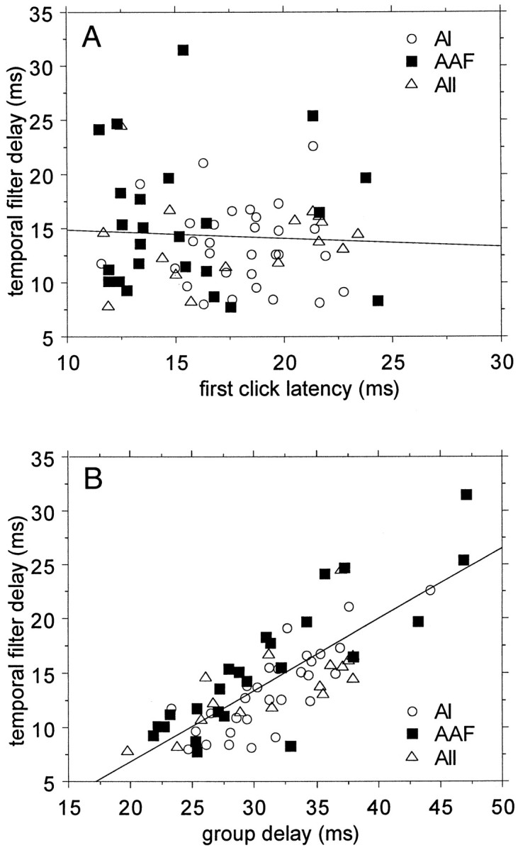
Dependence of the “temporal filter” delay on first click response latency and on group delay. A, The temporal filter delay for those units in which the group delay is at least 7.5 msec larger than the first click response latency is independent of the latency of the response to the first click.B, Strong correlation between the temporal filter delay (for the large delay subgroup) and the group delay.

Temporal modulation transfer functions and latency

The average tMTF for the groups with a difference in first click response latency and group delay of <7.5 msec had a smaller peak magnitude than that for the subgroup with latency difference >7.5 msec. Because of the potential of a third subgroup with filter delays >20 msec, an ANOVA of peak tMTF amplitude on three filter delay groups (delays <7.5, 7.5–20, and >20 msec) was performed and showed that the mean amplitude in the intermediate delay group was significantly larger than that for the small delay group (p < 0.0001) but not significantly different from the large delay group (p = 0.17). The small and large delay groups showed no significant difference either (p = 0.94). A linear regression analysis between BMF and temporal filter delay was performed per area and combined across areas. Across all areas the slope of the regression line (BMF = 7.61 Hz + 0.06 * filter delay) was not significantly different from zero. Calculated per individual area, the slopes of the regression lines were not significantly different from zero for AI and AII but showed a positive slope for AAF (BMF = 7.15 Hz + 0.11 * filter delay), which was significantly different from zero (p = 0.025). Because the temporal filter delays were indistinguishable in the three cortical areas, I assume that the finding of the small dependence between BMF and temporal filter delay in AAF has minimal implications. To explore this more systematically, mean tMTFs were constructed (magnitude and phase) for five subgroups differing by increments of 5 msec in the amount of cortical filter delay. Because there were no significant differences between cortical areas, the tMTFs were averaged across units from all areas. Figure5A shows that the largest magnitude (close to five spikes per click train) was found for the group with cortical filter delays of 15–20 msec. For filter delays >20 msec the magnitude was similar to that for the small filter delay groups. One observes that the best modulation frequency (peak of the magnitude function, BMF) is at 9.52 Hz, except for the 15–20 msec delay group, where it is 11.28 Hz. The limiting rate (the click rate for which the response magnitude is 50% of that at the BMF) was higher for the groups with filter delays of 10–15 and 15–20 msec than for the other groups. Figure 5B shows the mean phase plots for these groups, reflecting the increased group delay. In this representation the phase is expressed in degrees, and the click rate axis is logarithmic.

Fig. 5.

Magnitude and phase components of the mean tMTFs for subgroups of temporal filter delays. Results are shown for five subgroups. The subgroup with filter delay <5 msec comprised 142 units; the subgroup with filter delay from 5–10 msec comprised 38 units, the 10–15 msec filter delay group comprised 31 units; the 15–20 msec group comprised 22 units; and the group with filter delays in excess of 20 msec comprised 10 units. The magnitude function (A) is very similar for filter delays <10 and >20 msec, whereas the peak magnitude is larger for the subgroups with filter delays of 10–20 msec. The phase functions show the gradual increase in slope expected from this subdivision in temporal filter delays (B).

A subsequent regression analysis between the tMTF magnitude of the individual unit at every CRR and the value of the cortical filter delay (by cortical area) showed no significant dependence for CRRs <8 and >16 Hz. In the CRR region of 8–16 Hz there was a significant (p < 0.005) positive correlation between tMTF magnitude and cortical filter delay. In other words, with increasing magnitude the delay in this CRR range increased.

Of 106 multiunit recordings with at least two well separated single units, 69 recordings consisted of units that were all from the low filter delay group (<7.5 msec), 12 recordings comprised units with only large filter delays (>7.5 msec), and 25 recordings were composed of units from both groups. This percentage of mixed recordings (24%) is expected on basis of independence of finding low or high filter group units: the product of their occurrence rates in the overall population (0.70 and 0.30) predicts a 21% co-occurrence of recording them on the same electrode. This was not significantly different from the observed value.

Modeling the magnitude of the tMTF in terms of synaptic mechanisms

In Figure 6 the number of spikes per 10 clicks is presented as a function of the CRR for the five filter delay groups. This is an appropriate representation for estimating and discussing the synaptic depression and facilitation mechanisms responsible for the “adaptation.” Figure 6A shows that for all groups the functions are low-pass and have approximately the same shape. Curves based on twice smoothing the data are drawn in as well. Figure 6B presents the same data normalized on their mean response for CRRs between 1 and 4 Hz. One observes that for the groups with the 15–20 msec extra filter delay the CRR dependence has a different shape and, as observed before, shows an enhanced response in the 8–16 Hz range. The slope of the low-pass filter functions is for all groups steeper than 12 dB/octave and steepest for the 15–20 msec delay group.

Fig. 6.

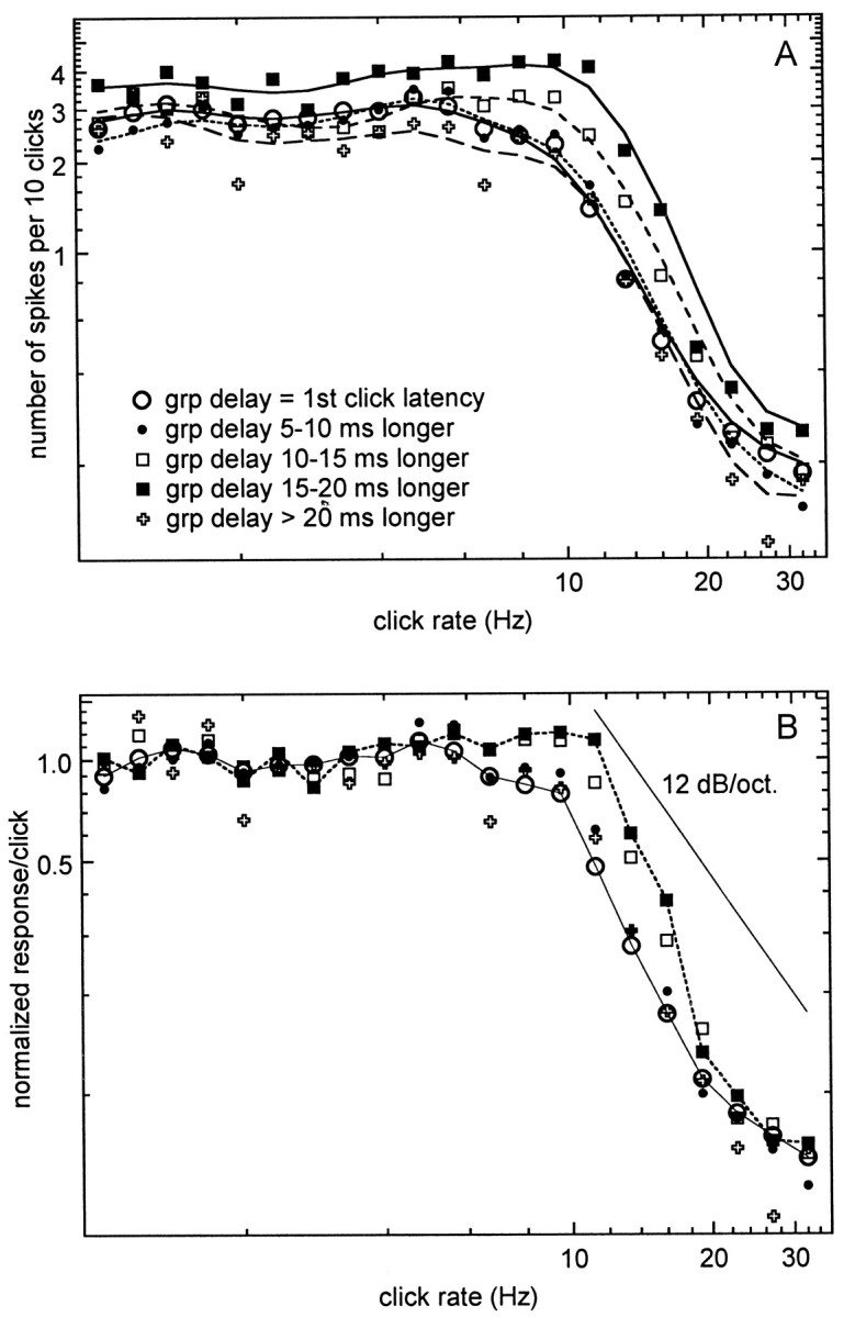
Adaptation functions expressed as number of spikes per click. A, These adaptation functions are low-pass functions of click repetition rate that have similar shape regardless of temporal filter delay. B, After normalizing the data on the mean values of the response between 1 and 4 Hz, the curves are similar, with the exception of the two groups with temporal filter delays between 10 and 20 msec. The high-frequency slope is steeper than 12 dB/octave.

For repetitive stimuli the model for the normalized steady-state response to a train with interstimulus interval, Δt, was given in Materials and Methods, and is repeated here for the summed response across the entire train:

$$R_{\text{av}}(\mathrm{\Delta }t)=[1-R(N\mathrm{\Delta }t){]}^N/[1-R(N\mathrm{\Delta }t)],$$ Equation 8A

and for the average response per click:

$$R_{\text{pc}}(\mathrm{\Delta }t)=R_{\text{av}}(\mathrm{\Delta }t)/(N+1).$$ Equation 8B

Recall that there is a multiplicative interaction between depression and facilitation, so that the response to the (N+ 1)th click becomes:

$$R(N\mathrm{\Delta }t)=[1-dexp(-\mathrm{\Delta }t/{\tau }_{\text{recov}}){]}^N[1+fexp(-\mathrm{\Delta }t/{\tau }_{\text{fac}}){]}^N,$$ Equation 9

The data-fitting procedure was done in Horizon, using the nonlinear least squares fitting procedure, which provides a χ² as an estimate of fit. To fit the data for the short filter delay group, the facilitation, f, was set equal to zero, and the amount of depression by a single click, d, and the recovery time constant was estimated. Introducing facilitation at this point only increased the χ², indicating a less acceptable fit. The 10–15 and 15–20 msec filter delay group tMTFs were subsequently modeled by introducing a small amount of facilitation, f, but leaving the other fit parameters the same as estimated for the short delay group. The results are shown in Figure 7, A and B. Figure 7A presents the tMTFs for the short delay group (open circles), the 10–15 msec delay group (open squares), and the 15–20 msec delay group (filled squares) on a linear ordinate, and Figure 7B presents the response per click on log-log scale. Without spontaneous activity, the model fitted the data well up to 13.44 Hz but for higher click rates underestimated the data. Introducing a small amount of spontaneous activity, identical for all click rates but slightly different for the three filter delay groups, made the model fit quite well. This residual activity may result from off responses that frequently are observed for the higher click rates and that were automatically incorporated in the calculation of the tMTF whenever they were within one interclick interval from the last click. The fit curves for the short filter delay group are shown with thefull lines (no facilitation, f = 0; strong depression, d = 0.9; fast recovery, τ_recov = 20 msec; spontaneous activity, 0.04 spikes per click), for the 10–15 msec delay group withwide-spaced dashed lines (f = 0.045; τ_fac = 60 msec; d = 0.9; τ_recov = 20 msec; spontaneous activity, 0.04 spikes per click), and for the 15–20 msec filter delay group with closely spaced dashed lines (f = 0.055; τ_fac = 60 msec; d = 0.9; τ_recov = 20 msec; spontaneous activity, 0.045 spikes per click).

Fig. 7.

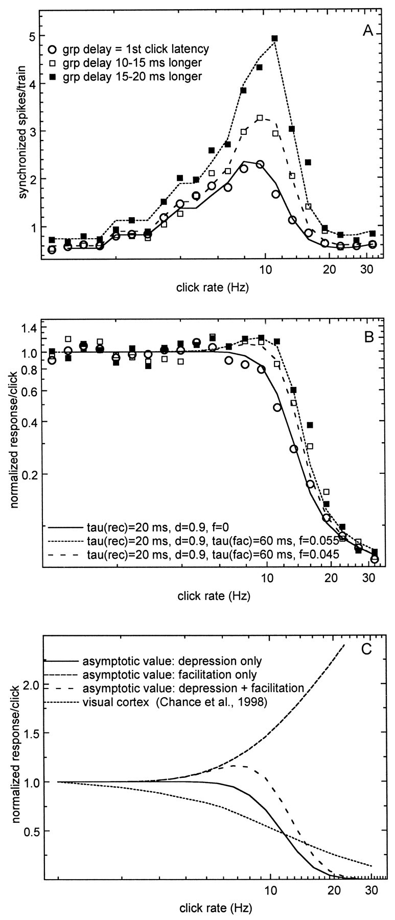
Modeling the magnitude of the tMTF on the basis of synaptic mechanisms. A, tMTFs for three groups of units together with the fit curves based on Equation 8A with the parameters shown in B. B, Adaptation functions together with the fit curves based on Equation 8B. C, Estimates of the asymptotic adaptation functions (for 30 clicks) for depression, facilitation, and the combination thereof. For comparison an adaptation function for visual cortex is shown.

These fit curves are for average values per filter delay group. Figure3 showed that for each group there is a large range of peak tMTF amplitude values. This variation reduces the amplitude range by a factor of 30 (∼1.5 log unit) when the peak amplitude is normalized on the average firing rate for CRRs between 1 and 4 Hz. This suggests that the overall firing rate of the units is a major factor in this variation. For the group with filter delays in the 10–20 msec range the variation in peak amplitude can be further explained by a small variation in the amount of facilitation. For instance, tMTFs with the largest amplitudes (1.25 log units or ∼18 synchronized spikes per click train) can be fitted by using f = 0.07. Forf = 0, the peak amplitude is approximately two spikes per train. To model individual unit tMTFs with smaller peak amplitude, for all filter delays, the depression time constant has to be increased slightly. For instance, an increase to 24 msec is sufficient to fit a tMTF with a peak amplitude of 0.5 spikes per train. However, the overall variation found in the number of synchronized spikes per train for low CRRs, which accounts for at least half of the variation in the peak amplitude, cannot be explained by changes in the amount of short-term depression or facilitation.

These model results suggest that the recovery time constant for the auditory cortex is approximately a factor of 4 smaller than for other neocortical areas and that relatively small amounts of synaptic facilitation can account for most of the observed quantitatively large tMTF magnitude changes for the various temporal delay groups.

The model parameters can in turn be used to generate asymptotic values for a constant number of clicks in the train instead of a constant train length. In Figure 7C the asymptotic values after 30 clicks are shown for depression only (Eq. 5B; time constant, 20 msec), for facilitation only (Eq. 6; time constant, 60 msec; 5.5% facilitation), and for depression and facilitation combined (Eq. 9). Note the enhancement between 3 and 10 Hz. For comparison, model data for visual cortex cells under periodic stimulation (Chance et al., 1998) are shown as well.

Local field potentials

For the simultaneously recorded LFPs, magnitude tMTFs, onset latency, and group delay measurements were obtained in the same way as for the single units. As shown previously, the magnitude tMTF for LFP triggers is, save for a scale factor, identical to those for simultaneously recorded units (Eggermont and Smith, 1995), suggesting that the tMTF magnitude is determined at the input level to the neurons. Figure 8 shows some comparisons between LFP and SU measures for onset latency and group delays, suggesting that factors contributing to the SU filter delays are acting at the spike generation level. Figure 8A presents latency of the response to first clicks for SU as a function of that for LFP triggers for the low and high filter delay category for the SUs. The slopes of the regression lines for the two groups are not significantly different, and neither is significantly different from one. Thus LFP latencies to first clicks are highly predictive of the SU latencies to first clicks. Figure 8B compares the group delays for LFPs and SU spikes. One observes that there still is a good correlation for the small filter delay group but no correlation for the high filter delay group. In the latter group the mean group delay difference between SU and LFP is 14.5 msec. This suggests that the extra delay for the SU arises at the spike generation level and not from the specific afferent input to the neurons.

Fig. 8.

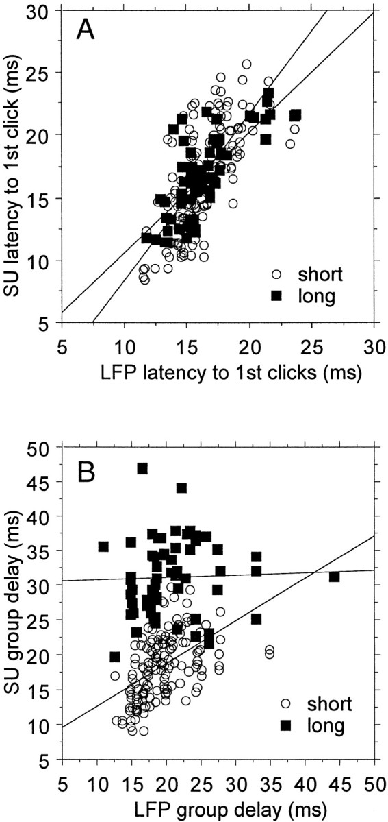
Relationships between LFP and single-unit latencies for first click responses (A) and for group delays (B). There is a close correlation for first click latencies across both filter delay groups. For the group with short temporal filter delays, the two estimates of group delay are correlated, but there is no correlation between LFP and SU group delays for the long SU temporal delay group.

DISCUSSION

For approximately two-thirds of the 215 single units the group delay calculated from the phase–MF dependence was within 7.5 msec of the response latency to the first clicks in the trains. For the remaining one-third of the units, the group delay was on average ∼14 msec higher. The overall amplitude distribution is unimodal and has higher values for filter delays in the 10–20 msec range. These findings were similar in the three cortical areas. Schulze and Langner (1997) compared group delays in primary auditory cortex to AM tones with latencies to unmodulated tone burst and found a similar dependence as in the present study. The difference in group delay and first click latency is interpreted here as a temporal filter delay. For intermediate values of the temporal filter delay an enhancement of the magnitude of the tMTF was observed, resulting in increased limiting rates. This enhancement was the same for units and LFPs. For the long delay group, the temporal filter delay for single units was ∼14.5 msec longer than for LFPs, suggesting that the temporal filter delay is related to spike generation.

Systems analysis

The differences between the various filter delay groups can be elucidated by comparing the average magnitude and phase of the tMTF for the low (<7.5 msec) and high (>7.5 msec) filter delay groups (Fig.9A,B) and calculating the magnitude ratio and phase shift between the two groups (Fig.9D,E). As suggested above, the additional phase shift only occurs at >8 Hz, and the extra magnitude gain occurs largely between 8 and 16 Hz. The impulse responses for the low and high filter delay groups, calculated by inverse Fourier transformation of the complex spectrum, formed by combining the magnitude and phase data, are shown in Figure 9C and indicate the peak latencies expected from the group delays for the two groups. The extra gain and phase shift, needed to convert the tMTF of the low filter delay group into the high delay tMTF, shown in Figure 9, D and E, can be interpreted as resulting from the action of an “amplifying filter” with impulse response shown in Figure 9F. The nature of the filter is not immediately obvious. Generally, increased group delays correspond to steeper filters, which does not fit the increase in the magnitude of the tMTF with increasing group delay, unless an amplification aspect is introduced. This amplification could be akin to that observed in reducing the damping of a bandpass system. Concurrent with the increase in output at the “resonant” frequency, the phase change is more rapid across the frequency range of the peak response than for a more damped resonator (Bendat and Piersol, 1971). The group delay introduced by a filter with otherwise the same characteristics would thus be much larger in the more resonant, less damped, filter. In our data the observed phase changes are of the order of 2π–3π radians, and the slope of the tMTF filter is ∼18–24 dB/octave, suggesting that the filter is of approximately fourth order.

Fig. 9.

Magnitude (A) and phase (B) for the group with filter delay <7.5 msec (*) and that with longer filter delays (○). The corresponding impulse responses are shown in C. D,E, Magnitude ratio and phase shift between the two groups, which can be interpreted as the action of an amplifying filter with impulse response, as shown in F.

For LFPs, filter delays were also split into two groups; however, the vast majority showed a delay that was <5 msec. The SU filter delays were independent of the LFP filter delays; for the short filter delay group the mean difference was 1.5 msec, and for the long delay group it was 14.5 msec. This suggests that the long group delays for the SU are the result of effects additional to those for the EPSPs of which the LFPs are an extracellular representation (Mitzdorf, 1985; Varela et al., 1997). The finding of an independent distribution of units belonging to the two temporal delay groups suggests that the explanation for the long filter delays is in individual, not spatially segregated, neuron properties. The observation that the distribution of low and high filter delay neurons is similar in all three cortical areas corroborates this.

After the subdivision of the population into groups of ascending temporal filter delay in 5 msec steps, the groups with filter delays between 10 and 20 msec stand out as a separate group with enhancement of the tMTF. The group with larger delays had a tMTF similar to that for the groups with temporal filter delays <10 msec. Putting the separation boundaries at 7.5 and 20 msec made no difference in the findings. This suggests that the temporal filter is not a minimum phase system, with its unique relationship between the magnitude and the phase functions of the tMTF, allowing one to be calculated from the other (Papoulis, 1977). The linearity of the phase–CRR dependence suggests that it can be treated as a system that results in a pure delay for the neural responses. This delay is likely the result of cumulative effects of depression and recovery mechanisms. The enhancement in the tMTF magnitude can be seen as resulting from an independent mechanism, notably presynaptic facilitation.

Modeling on the basis of synaptic mechanisms

The observed enhancement in the magnitude of the tMTF could be explained by a modest amount of facilitation. This puts the amplification at the input site of the neuron. Previous findings (Eggermont and Smith, 1995) that the LFP-based tMTF is a scaled version of those for SU and MU also suggest this. Initially, the tMTFs were fitted using time constants for visual cortex neurons. Modeling the data using the published adaptation time constant of 33 msec and the recovery time constant of 80 msec (Wang, 1998) required also 90% facilitation with a time constant of 87 msec, comparable to what was reported for visual neurons (Varela et al., 1997) to obtain some resemblance to the tMTF. This did, however, not result in an acceptable fit to the data, because the residuals were not spherically distributed, and the steep decrease for CRR could not be obtained. The next step, as described in Results, was to assume very little facilitation as is common for neocortical cells (Markram et al., 1998) and to estimate the time constants by a least mean squares curve-fitting procedure. The best results for the short filter delay group (Fig. 7) were obtained with a model that provided a short adaptation time constant of 8 msec, a short recovery time constant of 20 msec, ∼90% of depression, and no facilitation. It was impossible to obtain a good fit for the tMTFs in the 10–20 msec filter delay groups without incorporating a small amount of facilitation. A multiplicative combination of effects of previous stimuli, for depression as well as facilitation, was the only way to obtain a good fit to the data. The variance in the response for low CCR, which accounts for up to half of the variance at the tMTF peak, cannot be explained by this model.

Comparison with other studies

The decrease in the number of spikes per click as a function of click rate can theoretically (see Materials and Methods) be described by three time constants, τ_adap, τ_fac, and τ_recov. The adaptation time constant, τ_adap, reflects fast adaptation properties and was identified by Wang (1998) as depending on the [Ca²⁺] extrusion and buffering properties of the neuron, quantified by τ_Ca, and on the product of the spike-evoked [Ca²⁺] influx size and the conductance of the afterhyperpolarization. Differences in adaptation (τ_adap values from 10 to 50 msec) for pyramidal cells in visual cortex have been reported for superficial and deep layers (Ahmed et al., 1993). In the model a value as short as 8 msec was needed. As a result of this very short perstimulatory adaptation time constant the fraction of depression introduced by a single click was 0.94. This value is not unreasonable in light of the very short transient response of cells in auditory cortex to a single click, which typically consists of one to three spikes within 10 msec, followed by a 60–150 msec period of suppressed spontaneous activity. The recovery time constant for visual cortical cells, τ_recov, was considered by Wang (1998) to be solely dependent on τ_Ca and to be smallest in the dendrites (80 msec) and much larger for the soma (240 msec). Our tMTFs and adaptation functions could only be fitted using a recovery time constant that was approximately four times smaller than the one used by Wang (1998) for the dendrites. Response facilitation has also been demonstrated in neocortex, especially under low quantal release conditions (Varela et al., 1997). A small amount of facilitation, <7%, in agreement with values for neocortical cells (Markram et al., 1998), appeared to explain most of the changes in the magnitude of the tMTF. For visual neocortical synapses (Varela et al., 1997) the facilitation time constants were somewhat larger (90–120 msec) than the 60 msec obtained from our curve fit procedure.

This model result indicates that auditory cortical cells may have much faster recovery mechanisms than visual cortical cells on which previous temporal modeling was based (Varela et al., 1997; Chance et al., 1998;Wang, 1998). This fast recovery may be required for the ability of the auditory cortex to reliably track the fast amplitude modulations that occur in natural sounds.

REFERENCES

- 1.Ahmed B, Anderson C, Douglas RJ, Martin KAC. A method of estimating net somatic input current from the action potential discharge of neurones in the visual cortex of the anaesthetized cat. J Physiol (Lond) 1993;459:134. [Google Scholar]
- 2.Anderson DJ, Rose JE, Hind JE, Brugge JF. Temporal position of discharges in single auditory nerve fibers within the cycle of a sine-wave stimulus: frequency and intensity effects. J Acoust Soc Am. 1971;49:1131–1139. doi: 10.1121/1.1912474. [DOI] [PubMed] [Google Scholar]
- 3.Bendat JS, Piersol AG. Random data: analysis and measurement procedures. Wiley; New York: 1971. [Google Scholar]
- 4.Chance FS, Nelson SB, Abbott LF. Synaptic depression and the temporal response characteristics of V1 cells. J Neurosci. 1998;18:4785–4799. doi: 10.1523/JNEUROSCI.18-12-04785.1998. [DOI] [PMC free article] [PubMed] [Google Scholar]
- 5.Eggermont JJ. Peripheral auditory adaptation and fatigue: a model oriented review. Hear Res. 1985;18:57–71. doi: 10.1016/0378-5955(85)90110-8. [DOI] [PubMed] [Google Scholar]
- 6.Eggermont JJ. Rate and synchronization measures of periodicity coding in cat primary auditory cortex. Hear Res. 1991;56:153–167. doi: 10.1016/0378-5955(91)90165-6. [DOI] [PubMed] [Google Scholar]
- 7.Eggermont JJ. How homogeneous is cat primary auditory cortex? Evidence from simultaneous single-unit recordings. Aud Neurosci. 1996;2:76–96. [Google Scholar]
- 8.Eggermont JJ, Smith GM. Synchrony between single-unit activity and local field potentials in relation to periodicity coding in primary auditory cortex. J Neurophysiol. 1995;73:227–245. doi: 10.1152/jn.1995.73.1.227. [DOI] [PubMed] [Google Scholar]
- 9.Gillespie DT. Markov processes. An introduction for physical scientists. Academic; Boston: 1992. [Google Scholar]
- 10.Magleby KL. Short term changes in synaptic efficacy. In: Edelman G, Gall W, Cowan W, editors. Synaptic function. Wiley; New York: 1987. pp. 21–56. [Google Scholar]
- 11.Markram H, Wang Y, Tsodys M. Differential signaling via the same axon of neocortical pyramidal neurons. Proc Natl Acad Sci USA. 1998;95:5323–5328. doi: 10.1073/pnas.95.9.5323. [DOI] [PMC free article] [PubMed] [Google Scholar]
- 12.Mitzdorf U. Current source-density method and application in cat cerebral cortex: investigation of evoked potential and EEG phenomena. Physiol Rev. 1985;65:37–99. doi: 10.1152/physrev.1985.65.1.37. [DOI] [PubMed] [Google Scholar]
- 13.Papoulis A. Signal analysis. McGraw-Hill; New York: 1977. [Google Scholar]
- 14.Ruston H, Bordogna J. Electric networks: functions, filters, analysis. McGraw-Hill; New York: 1986. [Google Scholar]
- 15.Schreiner CE, Langner G. Coding of temporal patterns in the central auditory nervous system. In: Edelman G, Gall W, Cowan W, editors. Auditory function. Neurobiological bases of hearing. Wiley; New York: 1988. pp. 337–361. [Google Scholar]
- 16.Schulze H, Langner G. Perioducity coding in the primary auditory cortex of the Mongolian gerbil (Meriones unguiculatus): two different coding strategies for pitch and rhythm? J Comp Physiol [A] 1997;181:651–663. doi: 10.1007/s003590050147. [DOI] [PubMed] [Google Scholar]
- 17.Varela JA, Sen K, Gibson J, Fost J, Abbott LF, Nelson SB. A quantitative description of short-term plasticity at excitatory synapses in layer 2/3 of rat primary visual cortex. J Neurosci. 1997;17:7926–7940. doi: 10.1523/JNEUROSCI.17-20-07926.1997. [DOI] [PMC free article] [PubMed] [Google Scholar]
- 18.Wang XJ. Calcium coding and adaptive temporal computation in cortical pyramidal neurons. J Neurophysiol. 1998;79:1549–1566. doi: 10.1152/jn.1998.79.3.1549. [DOI] [PubMed] [Google Scholar]
- 19.Zwicker H, Fastl H. Psychoacoustics. Facts and models. Springer; Berlin: 1990. [Google Scholar]