Finding the needle in the haystack: towards solving the protein-folding problem computationally

Abstract

Prediction of protein tertiary structures from amino acid sequence and understanding the mechanisms of how proteins fold, collectively known as “the protein folding problem,” has been a grand challenge in molecular biology for over half a century. Theories have been developed that provide us with an unprecedented understanding of protein folding mechanisms. However, computational simulation of protein folding is still difficult, and prediction of protein tertiary structure from amino acid sequence is an unsolved problem. Progress toward a satisfying solution has been slow due to challenges in sampling the vast conformational space and deriving sufficiently accurate energy functions. Nevertheless, several techniques and algorithms have been adopted to overcome these challenges, and the last two decades have seen exciting advances in enhanced sampling algorithms, computational power and tertiary structure prediction methodologies. This review aims at summarizing these computational techniques, specifically conformational sampling algorithms and energy approximations that have been frequently used to study protein-folding mechanisms or to de novo predict protein tertiary structures. We hope that this review can serve as an overview on how the protein-folding problem can be studied computationally and, in cases where experimental approaches are prohibitive, help the researcher choose the most relevant computational approach for the problem at hand. We conclude with a summary of current challenges faced and an outlook on potential future directions.

Introduction

Protein folding is a process of molecular self-assembly during which a disordered polypeptide chain collapses to form a compact and well-defined three-dimensional (3 D) tertiary structure. A grand challenge in biochemistry has been to understand the process by which proteins fold into their functional tertiary structure (folding mechanism) and to predict this tertiary structure from amino acid sequence (structure prediction), two tasks that are collectively known as “the protein-folding problem” (Chan and Dill 1993; Dill et al. 2008; Dill and MacCallum 2012). Solving this problem is of far-reaching impact as it will not only reveal the missing link between sequence and structure but also provide molecular biologists with a theoretical framework and practical tools for applications such as drug design and protein engineering. As a result, an enormous amount of effort has been contributed to study the protein-folding problem by the scientific community. This is illustrated by Figure 1, which shows the striking growth in the number of articles published each year on this problem since Anfinsen’s “thermodynamic hypothesis” of protein folding, that protein native state resides in the global minimum of Gibbs free energy, was formally stated in 1973 (Anfinsen 1973). A comprehensive review of the study of this problem is deemed impossible for an article of this kind. As many excellent review articles on the theories of protein folding and their experimental validation have been published over the years (Dill et al. 1995; Onuchic et al. 1997; Dobson et al. 1998; Dobson and Karplus 1999; Radford 2000; Onuchic and Wolynes 2004; Bartlett and Radford 2009; Bowman et al. 2011; Englander and Mayne 2014; Wolynes 2015), here we focus our discussion on computational methods for studying folding mechanisms and predicting tertiary structures. Specifically, we limit our discussion to protein-folding simulations and de novo protein structure prediction at atomic detail, as methods based on coarse-grained representation of protein structures were recently comprehensively reviewed (Kmiecik et al. 2016). In addition, due to space limitations, we are not able to cover the complete literature of this topic, and we apologize to those whose contributions have not received the deserved attention.

Figure 1.

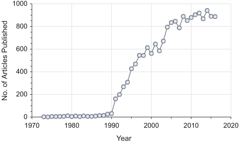
The number of articles published each year (1973–2016) with the phrase “protein structure prediction” or “protein folding” in either the title, or abstract or author keywords. The data were taken from web of science. A color version of this figure is available online (see color version of this figure at www.tandfonline.com/ibmg).

Nevertheless, the two key components of any folding simulation or structure prediction methods are efficient sampling of conformational space and accurate evaluation of the energy of sampled conformations. Hence, the main body of this article is devoted to discussing different algorithms and their advances toward efficient sampling of conformational space followed by approaches and progress toward accurate energy functions. To put the discussion under the theoretical framework of protein folding, we first briefly summarize different views on mechanisms of protein folding. The interplay between sampling algorithms and energy functions is concretely illustrated by discussing some representative methods shown to be relatively successful in the Critical Assessment of protein Structure Prediction (CASP) experiment (Moult et al. 1995; Tai et al. 2014). Finally, we present a summary on the progress and outline specific challenges that future development in the field will likely overcome.

Thermodynamics of protein folding

When a protein folds, it experiences constant counteractions between the effective energy, which favors the native state, and the configurational entropy, which favors unfolded states (Karplus 2011). The term “effective energy” refers to the free energy of the system (protein plus solvent) that consists of the intramolecular energy of the protein in vacuum plus the solvation free energy (the free energy of transfer of the protein from the gas phase to solution). The Gibbs free energy of the protein-solvent system is the sum of the effective energy and the configurational entropy (Lazaridis and Karplus 1999, 2000, 2003) (Figure 2). At equilibrium, both folded and unfolded states can be characterized by their Gibbs free energy. The difference in Gibbs free energies between the native state and unfolded states is termed the free energy of folding.

Figure 2.

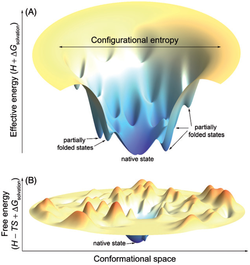
Schematic three-dimensional surface rendering of a hypothetical folding funnel diagram and a (Gibbs) free energy landscape to reference state. (A) A folding funnel diagram is a pictorial representation of the counteracting nature of the two thermodynamic variables, effective energy and configurational entropy, in protein folding and explains how the Levinthal paradox is resolved (Karplus 2011). The effective energy is plotted vertically and the configurational entropy horizontally. The funneled shape stems from the fact that the number of accessible configurations, which determines the configurational entropy, decreases as the native state of a protein is approached (Karplus 2011). (B) A free energy landscape maps between conformations and free energies. The global minimum on the landscape corresponds to the conformation of the native state and local minima correspond to partially unfolded states, which are separated by free energy barriers from the native state. Note that real free energy landscapes are high-dimensional and extremely rugged. A color version of this figure is available online (see color version of this figure at www.tandfonline.com/ibmg).

$$\Delta G_{\mathit{folding}}=\Delta H_{\mathit{folding}}-T\Delta S_{\mathit{folding}}+\Delta \Delta G_{\mathit{solvation}}$$ (1)

Both the enthalpic and entropic contributions to ΔG_folding mainly arise from intramolecular and protein-solvent nonbonded interactions and rearrangement of solvent molecules. As calculating the exact Gibbs free energy from first principles is prohibitive (Leach 2001), a simplified energy function is used in practical computer simulations of protein dynamics, folding and structure prediction. Broadly speaking, there are two different types of approaches to a simplified energy function. The first is a classical mechanical model that describes the potential energy, which is parameterized by analyzing the fundamental forces between particles; the second is a statistical model parameterized on data derived from statistical analysis of pair interactions and other properties in known protein structures (Lazaridis and Karplus 2000). In this review, we will use the term “energy” frequently when we discuss various implementations of energy functions for evaluating the “energy” of sampled conformations; however, the reader is advised to keep in mind that such energy approximations are not physically realistic Gibbs free energies.

Solvation can be accounted for by either immersing the protein into explicit solvent molecules or including in the energy function a term that implicitly models solvation free energy. The former approach is often adopted in molecular dynamics simulations and is desirable especially in cases where the purpose is to study structural details about protein–solvent interaction. Two major limitations of this approach are that the computational expense is high and the effective energy of a protein conformation is not known. The latter approach, often referred to as implicit solvation, is typically orders of magnitude faster and compatible with more sampling techniques than corresponding simulations with explicit solvent (Lazaridis and Karplus 2003).

Simulation of protein folding and tertiary structure prediction are very different subproblems

While both the prediction of protein tertiary structure and simulation of folding require efficient search of conformational space and accurate evaluation of the energy of sampled conformations, it needs to be emphasized that these two subproblems are rather different, with distinct solutions and limitations. Methods for tertiary structure prediction generally create 3D models by assembling small structural fragments or motifs, quite often, with physically unrealistic trajectory of conformational search and evaluate the energy of sampled conformations using statistical potentials. While this approach has worked quite successfully in creating models that are close to native structures (Bradley et al. 2005a; Zhang 2009; Moult et al. 2016), it has very little chance of giving insight into the mechanisms of folding. It is doubtless that if one could simulate actual folding processes, both subproblems would be solved. However, as will be explained in later sections, this is only possible for relatively small proteins using molecular dynamics simulations. Thus, methods for simulating folding mechanisms, while often employ physically realistic energy functions and can reveal important thermodynamics and kinetics about folding, are generally not useful for predicting structures for all but only small proteins.

Chemical kinetics of protein folding: mechanisms and pathways

The conformational space accessible to a polypeptide chain is astronomically large; a systematic search for the functional structure of a polypeptide chain with 100 residues would take an amount of time even longer than the age of the universe. The fact that proteins fold on a biologically meaningful timescale, with some attaining their functional structures in just a few microseconds, led Levinthal to conclude that there must be well-defined folding mechanisms and pathways to the native state (Levinthal 1968, 1969), so that protein folding is under “kinetic control.” A full characterization of the folding process requires elucidation of the mechanisms by which transition states and intermediates, if any, are formed and the determination of whether there is a single defined pathway or multiple pathways to the native state.

The “classical view” of protein folding assumes a sequential model and postulates a well-defined sequence of intermediates that follow one another to carry the protein from the unfolded random coil to a uniquely folded native state (Levinthal 1968; Kim and Baldwin 1982, 1990). In the search for such a single mechanism of protein folding, several models have been proposed about how folding gets started and native contacts and structure are subsequently formed (Baldwin 1989; Fersht 1997; Daggett and Fersht 2003a, 2003b). The “nucleation” model postulated that a folding-initiating local secondary structure, or nucleus, is formed slowly followed by the rapid propagation of native structure in a stepwise manner (Wetlaufer 1973). However, this model was dropped from favor as it predicts the absence of folding intermediates. The “framework” model and the related “diffusion-collision” model proposed that secondary structures segments are preformed independently of tertiary structure before they diffuse and collide to give stable tertiary structure (Kim and Baldwin 1990; Karplus and Weaver 1994). The “hydrophobic collapse” model hypothesized that folding starts with a rapid collapse around hydrophobic residues to the molten globule state (compact denatured state), that narrows down the conformational exploration to the native state significantly (Baldwin 1989; Ptitsyn 1996). An essential feature of these latter models is that they predict the presence of folding intermediates. However, the fact that some proteins fold by simple two-state kinetics, without the accumulation of folding intermediates, and that secondary and tertiary structure form simultaneously led to the formulation of the “nucleation-condensation” model (Fersht 1997; Daggett and Fersht 2003a, 2003b). This model assumed the concerted formation of local and nonlocal structures and was considered a “unifying” mechanism of protein folding (Daggett and Fersht 2003 b). It should be noted, however, that the “nucleation-condensation” model does not preclude the presence of folding intermediates (Daggett and Fersht 2003a, 2003b).

The observation that molten globules form asynchronously over a range of timescales fostered the concept of protein-folding funnel (Frauenfelder et al. 1991; Bryngelson et al. 1995; Dill and Chan 1997; Onuchic et al. 1997; Dobson et al. 1998; Brooks et al. 2001; Wolynes 2015) (Figure 2). In this “new view,” it is inferred that proteins must fold into their unique native state through multiple unpredictable pathways that involve the progressive organization of an ensemble of partially folded intermediates on a rugged effective energy hypersurface that resembles a funnel. The funnel shape arises from the fact that the number of accessible configurations, which determine the configurational entropy, decreases as the energy decreases (Karplus (2011). A more recent formulation of the mechanism of protein folding is centered around of concept of foldons (Englander et al. 2007; Englander and Mayne (2014). In what’s called the foldon-based hypothesis, a protein starts folding by forming an initial seed foldon through unguided search, and it follows a foldon-determined folding pathway as the seed foldon guides subsequent foldons in a “folding upon binding” way. While this hypothesis states that proteins fold along a definite path after formation of the initial foldon, the foldon formation at the initial stage is assumed to be accomplished through a disordered multitrack search (Englander and Mayne 2014).

Prediction of protein-folding rates

Folding rate is an essential parameter for characterizing protein-folding kinetics. What factors determine whether a protein will be a slow or fast folder? Can we predict folding rates from amino acid sequences as well? Theoretical studies have suggested that the size, native topology and stability of a protein influence the rate and mechanisms by which it folds. In searching for a causal relationship, a key advance made in 1998 was that in a set of 12 nonhomologous single-domain proteins folding rate shows a significant correlation with a simple measure of topological complexity of the native fold, the so-called contact order, which is defined as the average sequence separation between all pairs of native contacts normalized by sequence length (Plaxco et al. 1998). In contrast, the correlations between size or native state stability and folding rate are weak to nonexistent (Plaxco et al. 1998). Based on this observation, another parameter called long-range order, which counts long-range contacts (contacts that are close in space but distant in sequence), was proposed and found to be a strong predictor of the folding rates of two-state proteins (Gromiha and Selvaraj 2001). Contact order and long-range order have also been combined to form a parameter called total contact distance that has better correlation with folding rates (Zhou and Zhou 2002b). Folding rates were also found to be inversely correlated with a parameter called multiple contact index that measures the number of residues with multiple long-range contacts (Gromiha 2009). The correlations between the various topological parameters just discussed and folding rates suggest that it is viable to predict folding rates from amino acid sequences because native topologies are determined by amino acid sequences (Baker 2000). In fact, several bioinformatics tools have been developed for this purpose (Ivankov and Finkelstein 2004; Gromiha et al. 2006; Ouyang and Liang 2008; Chou and Shen 2009; Guo and Rao 2011), and two notable web servers are FOLD-RATE (Gromiha et al. 2006), FoldRate (Chou and Shen 2009).

Conformational sampling is a bottleneck

A polypeptide chain with a typical size can adopt an astronomical number of conformations. It is agreed that conformational sampling remains to be a bottleneck of de novo structure prediction (Jones 1997a; Baker and Sali 2001; Bradley et al. 2005b; Zhang 2008; Kim et al. 2009; Maximova et al. 2016). Nevertheless, there has been exciting improvement in sampling algorithms based on statistical mechanical principles or guided by experimental or predicted restraints, all of which are further accelerated by improvements in hardware speed and power (Maximova et al. 2016). For the convenience of discussion, we divide conformational search methods into the following three broad categories: molecular dynamics simulations, Monte Carlo simulations and genetic algorithms. For each category of algorithms, we give a general formulation of the algorithm and a summary of the latest studies in which the algorithm was applied to study protein folding mechanism or de novo protein structure prediction.

Unbiased molecular dynamics simulations

Molecular dynamics (MD) simulation is a widely used computational technique for exploring the macroscopic properties of molecular systems through explicit computation of microscopic particle motions. MD has had enormously influential applications in biomolecular systems and has been heavily used to study motion-related phenomena such as protein folding, conformational flexibility, protein structure determination from NMR, ligand–protein interaction and protein–membrane interaction (Karplus and Petsko 1990; van Gunsteren and Berendsen 1990; Karplus and McCammon 2002; Gumbart et al. 2005; Karplus and Kuriyan 2005; Lindahl and Sansom 2008; Klepeis et al. 2009; Durrant and McCammon 2011; Periole 2017). The two essential elements of an MD simulation are the interaction potential for the particles and the equations of motion governing the dynamics of the particles (Leach 2001; Rapaport 2004). Interaction potentials will be discussed in the section: Energy functions are evolving objects. Here, we describe how MD simulations explore the phase space of a molecular system.

A typical MD run involves generation of successive microstates of a molecular system by solving Newton’s equations of motion for all atoms simultaneously with femtosecond time steps (Equation (2)).

$$m_i\frac{d^2{\mathit{r}}_i}{{\mathit{dt}}^2}={\mathit{F}}_i=-\frac{\partial \mathit{U}({\mathit{r}}_1,{\mathit{r}}_2,\dots ,{\mathit{r}}_N)}{\partial {\mathit{r}}_i}$$ (2)

where r_i and U(r_1, r₂,…, r_N) denote position vector and potential energy of point mass i, respectively. F_i denotes the force acted upon point mass i. The result of the simulation is a trajectory of microstates that specify how the system evolves in phase space (Leach 2001). In principle, equilibrium properties can be computed by averaging over the trajectory if it is of sufficient length to give a representative ensemble of the microstates of the system. Unfortunately, the usefulness of MD in studying long timescale biological phenomena is often limited due to inadequate sampling of all relevant conformational states of a system. Even when the energy barriers separating two topologically different low-energy regions of the conformational space are of order k_BT, traversing them by random thermal fluctuation cannot be achieved within a reasonable amount of time.

A wide range of biologically interesting phenomena occurs over timescales in the order of milliseconds, several orders of magnitude beyond the reach of conventional MD simulations. As a result, studying processes that involve major conformational changes, such as protein folding, activation and deactivation, by MD simulations has been traditionally challenging (Gruebele 2002). The very first protein folding simulation via MD at the microsecond timescale was notably made by Duan and Kollman (1998), who simulated the folding process of the villin headpiece (a 36 mer) in explicit solvent for two months on parallel supercomputers. The simulation showed a mechanism for the peptide to reach a marginally stable state with a main chain RMSD of 5.7 Å from the native state (Duan and Kollman 1998). This peptide was later de novo folded by Zagrovic and coworkers (2002) to an ensemble of states whose average Cα RMSD is 1.7 Å from the native state. The total simulation time was 300 μs or approximately 1000 CPU years with the help of worldwide-distributed computers (Zagrovic et al. 2002).

Substantial progress has been made during the past decade or so to extend the folding times accessible by conventional MD simulations through efficient parallelization of MD codes or MD-specialized hardware (Lane et al. 2013) (Figure 3). The MD-specialized software package Desmond and the massively parallelized machine Anton, both developed recently at D.E. Shaw Research, have allowed for conducting millisecond timescale MD simulations of systems with tens of thousands of atoms in just a few weeks (Bowers et al. 2006; Shaw et al. 2007, 2014). Desmond is a collection of codes that implement novel parallel algorithms and numerical techniques to perform high-throughput and accurate MD simulations on conventional computational clusters, general-purpose supercomputers and GPUs (Bowers et al. 2006). Anton is built on MD-specific ASICs (application-specific integrated circuits) that interact in a tightly coupled manner using a high-speed communication network. Its ability to efficiently perform simulations on the timescales over which many physiologically relevant processes take place expands the set of problems for which the use of MD is tractable (Shaw et al. 2007, 2014). Armed with this specialized set of software and hardware, researchers at D.E. Shaw Research have been able to simulate protein folding from extended random coils (Shaw et al. 2010; Lindorff-Larsen et al. 2011) and study structural origin of slow diffusion in protein folding (Chung et al. 2015), protein-ligand recognition (Dror et al. 2011; Shan et al. 2011), mechanism of nucleotide exchange in G proteins (Dror et al. 2015), and mechanisms of kinase activation and inhibition (Shan et al. 2014; Ingram et al. 2015) at realistic timescales. The de novo folding simulations conducted at D.E. Shaw Research generated computational insights in favor of the single-pathway view of protein folding (Figure 2). For example, equilibrium simulations of WW domain captured multiple folding and unfolding events that consistently follow a well-defined folding pathway (Shaw et al. 2010). However, subsequent folding simulations of 12 fast-folding proteins showed that although a majority of them fold along a single dominant route, differing “transition state classes” were observed for two proteins (Lindorff-Larsen et al. 2011).

Figure 3.

Folding time scales accessible to MD simulations have increased exponentially since Duan and Kollman used MD simulations in explicit solvent to study the process through which the villin headpiece reaches a marginally state (Duan and Kollman 1998). Shown are proteins simulated using unbiased, all-atom MD simulations in empirical force fields reported in the literature. Here, an accessible folding time scale is defined as one within which folding events are observed in MD simulations of folding from unfolded states. According to this definition, whether the ~10 ms folding time of ACBP is already accessible needs to be confirmed by further simulations as no folding events were observed in any of the trajectories used to construct a Markov state model of the ACBP-folding reaction (Voelz et al. 2012). Adapted, with permission, from reference (Lane et al. 2013). See reference (Lane et al. 2013) for reference to each folding simulation highlighted in the figure. A color version of this figure is available online (see color version of this figure at www.tandfonline.com/ibmg).

A different approach to overcome the sampling challenge of MD is through statistical analysis of multiple independent trajectories or aggregating independent short simulations using Markov state models (MSM) to make a complete model of system dynamics (Pande et al. 2010; Prinz et al. 2011; Lane et al. 2013). The MSM effectively pieces together this complete model from independent trajectories, allowing for prediction of kinetic phenomena on timescales much longer than the individual trajectories used to construct the model (Lane et al. 2013). While the MSM-based “multitrajectory” approach has some advantages over the reaction coordinate-based single trajectory analysis, such as identifying areas of phase space for adaptive sampling (Bowman et al. 2010, Weber and Pande, 2011), insights gained from MSM analysis does not always agree with the single-pathway view of folding. For example, while it was shown via single-trajectory analysis that folding of the WW domain follows a definite pathway where the first hairpin folds first (Shaw et al. 2010), a parallel statistically significant pathway where the second hairpin of the WW domain folds first was detected using MSM to analyze the same simulation trajectories (Lane et al. 2011). Similar analysis conducted on the MD trajectories of 12 small fast-folding proteins (Beauchamp et al. 2012), while showed that two-state model is inadequate for the same set of systems as described by a previous study (Lindorff-Larsen et al. 2011), revealed a richer picture of populated states for some more complicated systems.

Enhanced sampling techniques in MD

The ruggedness of energy landscapes with many local minima separated by high-energy barriers makes adequate conformational sampling a challenging task. MD trajectories often do not reach all biologically relevant conformations, a problem that can be addressed by employing enhanced sampling algorithms (Okamoto 2004; Bernardi et al. 2015). Two popular enhanced sampling techniques in the simulations of biological systems are replica-exchange molecular dynamics (REMD) and metadynamics (Bernardi et al. 2015). While we focus our discussion on the REMD along temperature, which is also known as parallel tempering, several variants of replica exchange protocols have also been reported (Fukunishi et al. 2002; Itoh et al. 2011; Wu et al. 2012).

The replica-exchange method was developed to overcome the multitude of local minima separated by high energy barriers (Sugita and Okamoto 1999). Many molecular simulation scenarios require ergodic sampling of energy landscapes that feature many minima, and barriers between minima can be difficult to overcome at ambient temperatures over accessible simulation timescales. Replica-exchange simulations seek to enhance the sampling in such scenarios by running n non-interacting copies of the system C_i (i = 1, …, n) in parallel each at a different temperature T_i in the canonical ensemble (Figure 4). The non-interacting nature of this artificial compound system (C₁, C₂, …, C_n) ensures that each state’s weight factor is given by the product of Boltzmann factors of each copy.

Figure 4.

A sketch of the process of REMD and that of metadynamics. REMD: a set of noninteracting replicas (T1 through T4 in this illustration), each runs at a different temperature. Each color represents a single replica. As the simulation proceeds, each replica walks up and down in temperature. In an efficient REMD, replicas at neighboring temperatures are swapped (shown as double-headed arrows) based on Metropolis criterion and all replicas will experience swapping. Metadynamics: this illustrative system has two minima A and B (gray curve). The system trapped in B is lifted by progressive deposition of repulsive Gaussian kernels (green curve) and the free energy landscape changes accordingly (blue dashed curve). After B is filled up, the system moves into A which is filled up similarly. When the simulation completes, the green curve gives a first rough negative estimate of the free energy landscape of the system. A color version of this figure is available online (see color version of this figure at www.tandfonline.com/ibmg).

$$w=\text{exp}\left\{-\sum _{i=1}^n{\beta }_i{U}_i\right\}$$ (3)

Compared to a standard Monte Carlo simulation, which affects the conformation of only one copy, REMD explores the energy landscape by periodically exchanging the conformations of replicas. The probability of transition of a compound system such that the conformations between a pair of copies (C_i, C_j) are exchanged is

$$p=\text{min}(1,e^{\Delta })$$ (4)

where

$$\Delta =({\beta }_j-{\beta }_i)(U_j-U_i)$$ (5)

In most cases, exchange of the conformations of replicas decreases auto-correlation, thus enabling replicas to reach thermal equilibrium faster than without exchange. However, for protein folding simulation, a recent study showed that the efficiency of REMD is not much higher than that of conventional MD if the folding rate is not very temperature-dependent (Rosta and Hummer 2009). While it is not necessary to restrict the exchange to copies with neighboring temperature (e.g. j=i+ 1), doing so will be optimal, since the transition probability decreases exponentially with the difference in temperature between copies (Hansmann 1997). It is also worth noted that while exchange of conformations between copies must be conducted in a Monte Carlo way, there is no restriction on which algorithms are used for updating the conformation of an individual copy locally. In fact, several variants of REMD have been developed (Mori et al. 2016). For example, a replica-exchange Monte Carlo (REMC) technique was implemented in the threading-based structure prediction pipeline QUARK and tested in CASP11 (Zhang et al. 2016).

Metadynamics is a class of methods that eases sampling by introducing a time-dependent biasing potential that acts on a selected number of coarse-grained order parameters, often referred to as collective variables (CVs) (Laio and Parrinello 2002; Piana and Laio 2007; Barducci et al. 2011; Valsson et al. 2016). CVs are generally nonlinear functions of the atomic positions of the simulated system that should ideally distinguish between all relevant metastable states. Some simple but informative CVs used in protein-folding simulations are number of Cα contacts, number of backbone H-bonds and helicity of the backbone and the free energy surface is usually plotted as a function of these CVs (Piana and Laio 2007). The added biasing potential is introduced through successive addition of small repulsive Gaussian kernels deposited along the system trajectory in CV space (Figure 4) (Barducci et al. 2011; Valsson et al. 2016). The added Gaussian kernel is a function of the current position and the previous position of the system in the CV space, and its intended purpose is to discourage the system from revisiting configurations that have already been sampled, thus accelerating sampling. The final summation of the deposited Gaussian kernels also gives an unbiased estimate of the free energy landscape of the system. In contrast to these advantages, it is, however, far from trivial to decide when to stop a simulation and find a set of CVs proper for describing the process of interest (Barducci et al. 2011; Valsson et al. 2016).

Both REMD and metadynamics have been used to de novo fold several small peptides and proteins. The first example of using REMD to sample a folded structure starting from a completely unfolded state is probably the study of Rhee et al. (Rheeand Pande 2003) where a 23-residue BBA5 protein was folded by what’s called multiplexed REMD. Using REMD simulations in implicit solvent, Pitera et al. (Pitera and Swope 2003) folded a 20-residue designed Trp-cage peptide starting from an extended coil to a state <1.0 Å Cα RMSD from conformations in the NMR ensemble. Recently,Jiang etal.(JiangandWu2014)foldedadiverseset of 14 fast folding proteins from their unfolded states using REMD with a residue-specific force field. A similar study by Nguyen et al. (Nguyen etal. 2014) included a larger set of 17 proteins;while they successfully folded most proteins, mis-folded structures are thermodynamically preferred for 3 proteins.

Monte Carlo simulation

MD simulation is without a doubt a required technique if one wishes to study folding pathway or kinetics computationally. However, for tertiary structure prediction of large proteins whose energy landscapes are populated with many local minima separated by high barriers, Monte Carlo (MC) simulation can be much more efficient (Figure 5(A)). It is, in fact, the underlying search engine of some of the most successful de novo tertiary structure prediction methods (Simons et al. 1997; Bradley et al. 2005a; Xu and Zhang 2012; Zhang et al. 2016) and our method BCL::Fold (Karakas et al. 2012). Unlike MD simulations where successive conformations of the system are connected through time, in a MC simulation, each new conformation of the system depends only upon its immediate predecessor. The technique of MC simulation was introduced as the first computer simulation of a molecular system in 1952 (Metropolis et al. 1953). Nowadays, the term “Monte Carlo” is often used to describe a simulation whenever random sampling is performed.

Figure 5.

Monte Carlo simulated annealing and genetic operations in genetic algorithms. (A) A Monte Carlo simulated annealing procedure allows the system to “freely” navigate on the free energy surface. For example, transition from state 4 to 5 would be prohibitive to MD simulations due to the high-energy barrier separating them. (B) In genetic algorithms, conformations are encoded as bit strings (or real-valued arrays) called chromosomes. A mutation operation flips the bit value at a randomly selected site, whereas a crossover operation takes a pair of chromosomes and exchanges parts of chromosomes split at a randomly selected crossover site. A color version of this figure is available online (see color version of this figure at www.tandfonline.com/ibmg).

A MC simulation explores the phase space of a system by randomly perturbing the current conformation by actions such as moving a single atom or molecule or adjusting dihedral angles. The energy of the new conformation is then evaluated using an energy function. If the new conformation is lower in energy than its predecessor, it is accepted as a starting conformation for the next iteration. If the energy is higher, the new conformation is accepted with a probability based on the famous Metropolis criterion (Metropolis et al. 1953) (Equation (4). This is often done by comparing the Boltzmann factor of the new conformation to a random number between 0 and 1, and the new conformation is accepted if its Boltzmann factor is greater than the random number and rejected otherwise. While the essential search algorithm of MC-based structure prediction methods is the same, they differ in the starting components for assembling 3 D models and in the repertoire of MC moves implemented for perturbing the model (Vitalis and Pappu 2009).

Primitive MC sampling can be computationally expensive and thus inefficient at finding global energy minimum. Typically, these methods are coupled with some optimization technique that vastly decreases computational expense by directing the progression of the MC simulation toward global energy minimum. One optimization technique is gradient-based sampling, where MC iterations are directed down local property gradients, that is, the potential next state with the lowest energy is selected. For instance, gradients can be calculated based on side-chain rotameric states (Hu et al. 2010) or, in the HP-lattice model (Dill et al. 1995), the movement of a residue in various directions (Hu et al. 2009). However, when the conformational space is continuous rather than discrete, gradient descent becomes unfeasible because the energy cannot be calculated for every step forward. The most popular optimization approach shown to effectively accelerate the convergence of a MC simulation is probably simulated annealing (Kirkpatrick et al. 1983). The essential feature of this technique is that it combines MC sampling of conformational space at an initially elevated temperature with a proper cooling scheme over the course of the simulation. The cooling scheme, if gentle enough, theoretically ensures the system will reach the global minimum. In turn, the probability of a higher energy step being accepted decreases over time, and models are directed toward the global energy minimum (Tsallis and Stariolo 1996). Many powerful de novo tertiary structure prediction methods integrate this MC-simulated annealing approach (Kmiecik et al. 2016); we include a detailed discussion on some selected examples of such methods (see Examples of methods for de novo tertiary structure prediction).

Genetic algorithms

Genetic algorithms (GAs) are an optimization procedure based on the process of evolution that occurs in nature. GAs have been used in a variety of applications. Some prominent ones include automatic programing, machine learning and population genetics (Goldberg 1989). Generally, a GA initializes the optimization process by randomly generating an initial population of trial solutions each encoded as a string of bits, also called a chromosome (Figure 5(B)). Offspring are produced by applying nature-inspired operations, namely mutations and crossovers on bit strings. Mutations are introduced into strings by flipping one or more bits, whereas crossovers between two individuals consist of randomly selecting a crossover site and exchanging the left segment of one string with the right segment of the other (Figure 5(B)). The fittest offspring are selected for continual refinement via the iteration of multiple generations (Schulze-Kremer 2000).

A large number of studies on the use of GAs for de novo protein structure prediction and protein folding simulation have been made (Pedersen and Moult 1996; Cui et al. 1998; Schulze-Kremer 2000; Custodio et al. 2004; Unger 2004; Hoque et al. 2009; Huang et al. 2010; Zhang et al. 2010; Custodio et al. 2014; Boskovic and Brest 2016; Rashid et al. 2016) since the pioneering work of Dendekar and Argos (Dandekar and Argos 1992) on de novo folding simulation of a model protein of a four β-strand bundle and that of Unger and Moult (Unger and Moult 1993) on searching for global energy minimum on the 2D HP lattice model. The simplest protein representations used in GAs is the 2 D HP model developed by Lau and Dill (Lau and Dill 1989). In this model, amino acids are of only two types: hydrophobic (H) or polar (P). The sequence is folded on a 2 D square lattice on which bonds are orthogonal to each other. Folded structures are evaluated by a so-called “hydrophobic potential” where each pair of nonbonded direct hydrophobic contact (occupying neighboring nondiagonal lattice vertices) receives −1. Using HP lattice models avoids the computational cost needed for all-atom models while still capturing the general principles that govern protein folding, and they can be extended to account for physicochemical characteristics of individual residues such as size, hydrophobicity and charge. In more detailed models, proteins can be represented as a sequence of pairs of dihedral angles that describe the backbone degrees of freedom of each residue. Mutations can be introduced simply by changing the dihedral angle of a residue and crossovers by swapping randomly assigned sections of two sequences (Schulze-Kremer 2000; Unger 2004).

Energy functions are evolving objects

An essential part of almost all successful protein-folding simulations or protein tertiary structure predictions is an energy function that is a good approximation to the energy landscape of real proteins. Energy functions can be roughly divided into two classes: physics-based force fields and knowledge-based potentials (Lazaridis and Karplus 2000). Historically, physics-based forces fields are coupled with MD or MC simulations to study protein dynamics or calculate free energies (Wang et al. 2001; Ponder and Case 2003; Mackerell 2004; Lopes et al. (2015), whereas knowledge-based potentials are mostly used for fold recognition or tertiary structure prediction (Sippl 1995; Godzik 1996; Skolnick 2006). Before we give a detailed account on them, we remind the reader that both of these two types of energy functions are evolving objects. To improve accuracy, further parameter optimization for physics-based force fields is required and statistics need to be rederived for knowledge-based potentials when energy function deficiencies are identified or data sets of better qualities become available.

Physics-based force fields

Physics-based force fields are classical mechanical models that approximate the potential energy of chemical systems. Force field models ignore the electronic motions in a system and only consider interactions among nuclei. Compared to ab initio quantum mechanical methods, force fields are much more computationally efficient while giving an acceptable level of accuracy. A force field has a functional form and a (usually very large) set of associated parameters that, taken together, model bonded and nonbonded interactions in a system. The functional form of a force field is often a compromise between accuracy and computational efficiency and depends on the level of resolution (all atom or coarse grained), chemical nature (inorganic, small organic or biomolecular) and target properties of the systems to be modeled. Nevertheless, most force fields have five components (Equation (6)). The first three of them, so-called bond stretching, angle bending, and torsion, model bonded interactions. The last two components describe electrostatic and van der Waals nonbonded interactions (Leach 2001).

$$\begin{gathered} U({\mathit{r}}^N)=\sum _{\text{bonds}}\frac{k_b}{2}(l-l_0{)}^2+\sum _{\text{angles}}\frac{k_{\theta }}{2}(\theta -{\theta }_0{)}^2 \\ +\sum _{\text{torsions}}\frac{k_{\phi }}{2}\left[1+\cos (n\phi -\gamma )\right] \\ +\sum _{\text{electrostatics}}\frac{q_i{q}_j}{4\pi {\epsilon }_0{r}_{\mathit{ij}}}+\sum _{\text{VDW}}4{\epsilon }_{\mathit{ij}}\left[{\left(\frac{{\sigma }_{ij}}{r_{\mathit{ij}}}\right)}^{12}-{\left(\frac{{\sigma }_{ij}}{r_{\mathit{ij}}}\right)}^6\right] \end{gathered}$$ (6)

This functional form looks simple, but we must keep in mind that the set of parameters associated with it is very large. For example, the term that models bond stretching (a harmonic potential) has a different force constant k_b and an equilibrium bond length l₀ for each bond type. These parameters must be determined by fitting the force field to a given set of data obtained from experiments or quantum mechanical calculations. Depending on the size of the data set, parameter optimization may be conducted in a number of ways: trial and error, least-squares fitting (Lifson and Warshel 1968), or, recently, machine-learning algorithms (Behler (2016).

Well-known examples of force fields intended for modeling proteins include CHARMM (Gelin and Karplus 1979; Brooks et al. 1983; MacKerell et al. 1998, 2004; Brooks et al. 2009; Best et al. 2012), AMBER (Weiner and Kollman 1981; Weiner et al. 1984; Li and Bruschweiler 2010; Lindorff-Larsen et al. 2010), OPLS (Jorgensen and Tirado-Rives, 1988, Robertson et al. 2015), GROMOS (Van Gunsteren and Berendsen 1987; van Gunsteren et al. 1998), MARTINI (Marrink et al. 2007; Monticelli et al. 2008). These force fields were previously compared in-depth (Ponder and Case 2003), we note here that while the functional forms of these force fields invariably contain the five terms of Equation (6), some of them or their different versions may differ in specifics in the treatment of non-bonded interactions and the levels of resolution covered. For example, although more recent versions of the CHARMM and AMBER force fields do not model hydrogen-bonding energetics explicitly, originally CHARMM and AMBER force fields both incorporated a 12–10 Lennard-Jones potential to model hydrogen-bonding (Gelin and Karplus 1979; Weiner et al. 1984). The need for more efficient evaluation of nonbonded interactions arises when the number of interaction sites is large. One straightforward way to improve efficiency is to absorb aliphatic hydrogens into the carbon atom to which they are bonded to form “united atoms” as was done in the united-atom version of the CHARMM and OPLS force fields, or to use a coarse-graining approach where a group of heavy atoms are combined to form a representative virtual interaction site. The MARTINI force field aims at providing a simple model that is computationally fast and easy to use, and it adopted a “four-to-one” coarse-grain-ing scheme, meaning that on average four heavy atoms are represented by one interaction site (Marrink et al. 2007; Monticelli et al. 2008; Marrink and Tieleman (2013). Although all-atom simulations are often more desirable, if special care is taken during calibration of the building blocks and parameterization, a level of accuracy comparable to all-atom simulations may be possible in reproducing some thermodynamic properties with reduced representations while achieving considerable computational savings (Baron et al. 2006a, 2006b, 2007; Marrink et al. 2007; Monticelli et al. 2008; Marrink and Tieleman 2013). Coarse-grained protein models and their applications was recently reviewed in detail (Kmiecik et al. 2016).

Physics-based force fields are traditionally coupled with MD in simulating protein dynamics and folding (McCammon et al. 1977). There have been a plethora of such studies where the utility of force fields for protein tertiary structure prediction or the accuracy of reproducing experimental data were reported (Duan and Kollman 1998; Zagrovic et al. 2002; Pande et al. 2003; Summa and Levitt 2007; Lindorff-Larsen et al. 2011; Patapati and Glykos 2011; Lindorff-Larsen et al. 2012; Huang and MacKerell 2013; Piana et al. (2013). However, no agreement has been reached regarding whether force fields are sufficiently robust for these applications (Lee et al. 2009; Piana et al. (2014). Early analysis concluded that MD simulations under physics-based force fields are not particularly successful in structure prediction (Lee et al. 2009). However, for small, fast folding proteins that are also very stable, evidence has been accumulating that demonstrates that physics-based force fields are sufficiently accurate for predicting native-state structures and folding rates (Shaw et al. 2010; Lindorff-Larsen et al. 2011; Piana et al. 2012, 2013, 2014; Chung et al. (2015). In particular, it was pointed out the prediction of tertiary structures, folding rates and melting temperatures appears to be more robust than the prediction of the enthalpy and heat capacity of folding or that of the radii of gyration of unfolded states (Piana et al. 2014). It needs to be pointed out, however, that whether these force fields hold accurate for simulating larger proteins remains to be studied.

Knowledge-based potentials

Unlike physics-based force fields, which model interactions found in the most basic molecular systems using fundamental laws of physics explicitly and separately, knowledge-based potentials (KBPs) are energy functions derived from statistical analyses of known protein structures and the application of the inverse Boltzmann relation to the probability distribution of geometries (Wodak 2002; Sippl 1993, 1995). The physical meaning of KBPs has been under vigorous debate since their introduction (Finkelstein et al. 1995; Thomas and Dill 1996; Ben-Naim 1997; Moult 1997; Shortle 2003; Hamelryck et al. 2010), although justifications of KBPs as “potentials of mean force” have been provided by analogy to the reversible work theorem in statistical thermodynamics (Sippl et al. 1996) or on the basis of probabilistic arguments (Simons et al. 1997; Hamelryck et al. 2010). Nevertheless, KBPs are widely used and surprisingly effective in scenarios including but not limited to protein structure prediction (Simons et al. 1997; Lu and Skolnick 2001; Shen and Sali 2006; Xu and Zhang (2012), refinement of NMR structures (Kuszewski et al. 1996; Yang et al. 2012), fold recognition (Kocher et al. 1994; Majek and Elber 2009), protein–ligand or protein–protein interactions (Gohlke et al. 2000; Zhang et al. 2005; Huang and Zou 2006a; Huang and Zou 2006b) and protein design (Poole and Ranganathan 2006). Thus, in this article, we summarize the formalism of KBPs, specific implementations of different types of potentials, and their applications instead of concerning about the physical interpretation of KBPs.

A KBP energy function is a linear combination of individual potentials with each capturing a specific type of interaction. The most common formulation of such energy functions is as follows:

$$E(C\mid S)=\sum _{\mathit{ij}}{w}_{\mathit{ij}}\left(-\mathit{kT}\text{ln}\frac{p(c_j\mid s_i)}{p(c_j)}\right)$$ (7)

where E(C∣S) is the energy of conformation C given that the underlying amino acid sequence is S. p(c_j∣s_i) is the probability that a given sequence s_i adopts conformation c_j, whereas p(c_j) is an unconditional probability that any sequence fragment adopts conformation c_j· $\frac{p(c_j\mid s_i)}{p(c_j)}$ can be thought of as an “equilibrium constant” of a hypothetical chemical reaction: random sequence, unique conformation → unique sequence, unique conformation (Shortle 2003). In addition to the above inverse Boltzmann formulation, other formulations of individual KBP terms have also been widely used. For example, the KBP under the modeling package Rosetta was formulated based on the Bayes’ theorem (Simons et al. 1997). This approach was also adopted by Woetzel et al. recently to derive the KBP for a secondary structure element (SSE)-based protein structure prediction algorithm (Karakas et al. 2012; Woetzel et al. 2012; Weiner et al. 2013; Fischer et al. 2016). In their discrete optimized protein energy, or DOPE, Shen and Sali computed the negative logarithm of the joint probability density function of a given protein (Shen and Sali 2006).

The types of individual potentials incorporated into a KBP energy function are essentially only limited by the type of statistical relations that can be practically extracted from known protein structures. Depending on its intended purpose, a KBP may include individual potentials that fall into one or several categories. We elaborate three such potentials in the following and refer the reader to references (Simons et al. 1997; Woetzel et al. 2012; Xu and Zhang 2012) for examples of other potentials.

(1) Pairwise distance-dependent potential that approximates residue contact energies (Wodak 2002; Sippl, 1990, 1993, 1995). Such contact potentials are based on native inter-residue contacts that play a key role in determining folding kinetics and native state stability (Gromiha and Selvaraj 2004). The concept of pairwise distance-dependent potentials was first introduced in the pioneering work of Tanaka and Scheraga (Tanaka and Scheraga 1976), who related residue contact frequencies to the free energies of formation of corresponding interactions using the simple relationship between free energy and equilibrium constant. Their work was followed by that of Miyazawa and Jernigan (Miyazawa and Jernigan 1985, 1996), who formalized the theory of residue contact potentials using quasichemical approximation. However, these early implementations of contact potentials are not, in fact, distance-dependent, except that a single cutoff distance was used to define residue contact. A real pairwise distance-dependent potential was first introduced by Sipp (Sippl 1990), and this was followed by an explosion of different statistical potentials (Hendlich et al. 1990; Kocher et al. 1994; Park and Levitt 1996; Bahar and Jernigan 1997; Melo and Feytmans 1997; Park et al. 1997; Reva et al. 1997; Rooman and Gilis 1998; Samudrala and Moult 1998; Betancourt and Thirumalai 1999; Lu and Skolnick 2001; Zhou and Zhou 2002a; Fang and Shortle 2005; Qiu and Elber 2005; Summa et al. 2005; Dehouck et al. 2006; Shen and Sali 2006; Woetzel et al. 2012). Such pair potentials are usually formulated at residue level, where inter-residue distances are measured between C_β atoms or side-chain centroids in reduced representation of amino acid residues to promote computational efficiency. However, atomic-level formulation usually gives better discriminatory power albeit at the cost of more computational resource (Sippl 1996; Sippl et al. 1996; Melo and Feytmans 1997; Samudrala and Moult 1998; Lu and Skolnick 2001; Shen and Sali 2006).

(2) Solvent accessibility-based environment potentials that represent the interactions of individual residues with their local environment (Bowie et al. 1991; Kocher et al. 1994; DeLuca et al. 2011; Xu and Zhang 2012). Residue environment potentials are often included to account for solvation effects. Precise calculation of solvent accessibility requires full atomic structure and is time-consuming. In tertiary structure prediction scenarios where reduced representations of residues are used, good approximations to solvent accessibility, such as residue contact numbers, provide significant computational savings (Durham et al. 2009; Woetzel et al. 2012; Fischer et al. 2015; Li et al. 2016). It should be noted that in addition to transforming solvent accessibility statistics to energy-like potentials using the inverse Boltzmann relation, they have also been incorporated into KBP energy functions as a penalty term to disfavor models where residue-specific solvent accessibilities disagree with expected solvent accessibilities (Xu and Zhang 2012, Li et al. 2017).

(3) potentials of torsion angles that evaluate backbone φ, ψ torsion angles and/or the preference of side-chain rotamers (Kocher et al. 1994, Kuszewski et al. 1996, Betancourt and Skolnick 2004; Fang and Shortle 2005; Amir et al. 2008; Yang et al. 2012; Kim et al. 2013). It is well known that only certain combinations of φ, ψ torsion angles are populated in proteins (Ramakrishnan and Ramachandran 1965) and significant correlations exist between side-chain torsion angle probabilities and backbone φ, ψ angles (Dunbrack and Karplus 1993). Including such potentials has been shown to enable the energy function to exclude conformations that have unlikely combinations of torsion angles. In a study by Kocher et al. (Kocher et al. 1994) where several types of potentials were tested to recognize protein native folds, potentials representing backbone torsion angle preferences recognized as many as 68 protein chains out of a total of 74. This result was striking given the fact that backbone torsion potentials consider solely local interactions along the chain and are well known to be incapable of determining the full 3 D fold (Kocher et al. 1994). Potentials of torsion angles have also been used to refine structures generated from NMR data (Kuszewski et al. 1996, Yang et al. 2012). Kuszewski et al. (1996) incorporated a database-derived torsion angle potential into the target function for NMR structure refinement, resulting in a significant improvement in various quantitative measures of quality (Ramachandran plot, side-chain torsion angles, and overall packing. In a similar way, Yang et al. (2012) constructed a database of 2405 refined NMR structures.

Improving sampling and scoring with restraints

Due to their intrinsic inaccuracies, a common issue with energy functions is that incorrect conformations may be scored comparably to (or even better than) the native state (Skolnick 2006), lending the energy function inability to recognize the native state (Figure 6(A)). This issue be remedied by incorporating sparse experimental data as restraints, which offers some structural information that by itself is insufficient to completely determine the protein’s structure (Figure 6 (B,C)).

Figure 6.

Cooperative effects of energy functions and sparse restraints on a hypothetical protein. (A) the energy function has two comparable minima, lending itself the inability to tell decoy D1 from the native state N; (B) a scenario where decoy D1 violates some restraints and is thus penalized by the restraint score. However, as sparse restraints by themselves are insufficient to completely determine the protein’s structure, there exists decoys, such as D2, that satisfy the restraints as well as the native state N does; (C) Adding a restraint score to the energy function results in what’s called a pseudo-energy function which, in an ideal scenario, would be able to tell decoys apart from the native state; (D) the real free energy surface of the protein. A color version of this figure is available online (see color version of this figure at www.tandfonline.com/ibmg).

Sparse experimental data as restraints

Restraints from sparse experimental data drastically decrease the conformational space that needs to be sampled to only those structures consistent with the data. Many software suites implement algorithms to couple their de novo prediction methods with limited experimental data, including those from nuclear magnetic resonance (NMR), electron paramagnetic resonance (EPR), cross-linking mass spectrometry (XL-MS) and electron microscopy (EM).

NMR rivals X-ray crystallography as a technique by which an entire protein structure can be unambiguously determined. Solution-state NMR can determine the structure of relatively small proteins (< ~20kDa), but intensive experimental techniques and analysis of NMR spectra are required to determine a high-quality structure of a protein. Each residue typically requires upwards of 15 constraints. Oftentimes, NMR spectroscopy can provide some degree of low-resolution information about the global conformation of a protein, even for larger proteins (Venters et al. 1995; Battiste and Wagner 2000). These sparse restraints, including chemical shifts (CSs), nuclear overhauser enhancements (NOEs) and residual dipolar couplings (RDCs) do not provide enough information to fully determine the structure of a protein, but they can be used in conjunction with computational protein structure prediction software. CSs provide information about the protein backbone conformation, while NOEs and RDCs give information about the global fold of the protein. De novo protein structure prediction software can take advantage of just CSs (Latek et al. 2007), CSs and NOEs (Bowers et al. 2000) or all three types of restraints (Weiner et al. 2014).

Site-directed spin labeling (SDSL) and EPR can be used to glean information about proteins of nearly any size in their native environments. In addition, only a small amount of sample is required for structural interrogation by EPR. The accessibility and mobility of the spin labels can be used to determine the exposure and topology of SSEs (Farahbakhsh et al. 1992; Altenbach et al. 2005). Distances between spin labels can be detected up to 60Å and can give insight into the overall fold of the protein as well as different conformational states (Rabenstein and Shin 1995; Borbat et al. 2002). However, it is not feasible to use EPR to determine the full structure of a protein. EPR is experimentally intensive, as it requires the introduction of unpaired electrons at selected sites within proteins. This is usually done by cysteine substitution mutagenesis followed by modification of the sulfhydryl group with a nitroxide reagent. However, nonsense suppressor methodology, solid-phase peptide synthesis or “click-chemistry” have also been used (Klare and Steinhoff 2009). This technique will only give a small part of structural information about the protein, so these sparse EPR data can be used in conjunction with computational protein structure prediction methods (Alexander et al. 2008; Hirst et al. 2011; Fischer et al. 2015). The selection of sites to spin label is integral to the efficacy of structure determination by EPR (Alexander et al. 2008).

Similarly, XL-MS experiments can be used to determine interatomic distances that serve as experimental restraints. XL-MS can be used with proteins in their native states, and it has proven to be compatible with relatively large proteins, flexible proteins and membrane proteins (Kalkhof et al. 2005, Jacobsen et al. 2006, Lasker et al. 2012). In addition, the samples used can be heterogeneous and dynamic, as the output of XL-MS experiments is an average. The basis of XL-MS is the ability of two functional groups of a protein to form covalent bonds if they are within a certain distance of one another. These cross links can occur both inter- and intramolecularly. The proteins are then enzymatically digested, and MS is used to identify these cross links and surface labels (Young et al. 2000; Back et al. 2003; Sinz 2003).

EM provides data similar in format to that of X-ray crystallography, that is, a density map of a protein or complex. The data are thus less sparse than many of the aforementioned experimental techniques, but EM has historically provided lower-resolution density maps, from which an atomic structure cannot be gleaned. However, even low-resolution EM density maps are integral for identifying the overall organization of large molecular complexes. In recent years, EM technologies have progressed such that density maps with resolutions in the range of 4–8 Å can regularly be attained, at which level SSEs can be visualized and even some side-chain character can be visualized (Bihnstein and Melanie 2015). Many computational modeling methods have been developed that work with EM density maps (Lindert et al. 2009b), either in fitting previously solved structures into density maps, determining the topology and location of SSEs (Jiang et al. 2001; Abeysinghe et al. 2008), performing comparative modeling and de novo protein structure prediction (Lindert et al. 2009a, 2009c, 2012a, 2012b, 2012c; Woetzel et al. 2011).

Most de novo protein structure prediction algorithms require the use of a segmented density map, which can be accomplished with the use of various segmentation algorithms (Baker et al. 2006; Pintilie et al. 2010; Burger et al. 2011). Then, SSEs can be extracted from the density map either manually or with the use of algorithms that automate the selection of helices and/or sheets from a segmented density map (Jiang et al. 2001, Kong and Ma 2003; Kong et al. 2004; Baker et al. 2007). Next, de novo modeling algorithms can use these data with the density map and primary sequence of the protein in order to create a full structural model either via optimization (Chen et al. 2016) or using Monte Carlo methods (Lindert et al. 2012b, 2009c; Wang et al. 2015).

Predicted contacts as restraints

If no experimental restraints are available for the protein, secondary and tertiary structural restraints can be predicted from an amino acid sequence based on existing structures. Secondary structures can be predicted using machine learning methods. Artificial neural networks (ANNs) can be used to predict secondary structures from position-specific scoring matrices (Jones 1999; Yan et al. 2013), reduced amino acid representation (Leman et al. 2013), or multiple sequence alignments (MSAs) (Rost and Sander 1993a; Rost et al. 1993b). Methods have also been developed specifically to predict membrane protein topology from amino acid sequence using ANNs (Viklund et al. 2008; Viklund and Elofsson 2008; Leman et al. 2013), support vector machines (SVMs) (Nugent and Jones 2009), or Hidden Markov Models (HMMs) (Krogh et al. 2001; Kahsay et al. 2005).

It is a long-standing observation that 3D protein folds can be predicted from sufficient information regarding the protein’s inter-residue contacts (Gobel et al. 1994; Olmea and Valencia 1997; de Juan et al. (2013); the addition of even relatively sparse information about tertiary contacts into an algorithm’s scoring function can help improve protein models (Kim et al. 2014). Recently, the incorporation of long range contact predictions has resulted in some of the the most effective de novo protein structure prediction algorithms (Monastyrskyy et al. 2016; Moult et al. 2016). Several algorithms have been devised to predict these contacts using the principle of correlated mutations (de Juan et al. 2013). In general, amino acid contacts that stabilize the protein fold are assumed to evolve complementarily – if one residue of a contact is mutated, the other will likely also mutate to a reasonable interaction partner.

In order to identify pairs of correlated mutations, amino acid pairs can be scored based on their physicochemical similarity using the McLachlan matrix (McLachlan 1971), which is based on the frequencies of observed mutations in homologous proteins. Correlated mutations can also be scored by mutual information between MSAs based on the equation

$$\mathit{MI}=\sum _{\mathit{ab}}f(a_i{b}_j)\log \frac{f(a_i{b}_j)}{f(a_i)f(b_j)}$$ (8)

The above equation indicates that the mutual information between two protein sites i and j is computed by summing over amino acid pairs ab for every amino acid type a and b, where f(a_ib_j) is the observed relative frequency of ab at columns ij and f(a_i) is the observed relative frequency of amino acid type a at position i. The identification of these correlated mutations is used in many methods of multiple sequence alignment (Göbel et al. 1994; Neher 1994; Pollock and Taylor 1997; Ashkenazy and Kliger 2010; Hopf et al. 2014), from which tertiary contact predictions can be extrapolated.

In recent years, numerous algorithms have come out that account for covariance caused by indirect inter-residue coupling effects, which has led to improvement in prediction of correlated mutations (Burger and van Nimwegen 2010; Marks et al. 2011, 2012; Morcos et al. 2011; Jones et al. 2012b; Kamisetty et al. 2013; Skwark et al. 2013; Ekeberg et al. 2014; Hopf et al. 2014; Kaján et al. 2014; Michel et al. 2014; Ovchinnikov et al. 2014; Skwark et al. 2014; Jones et al. 2015). These methods were developed to resolve the issue that two residues aligned in multiple sequence alignments may exhibit statistical dependencies even though they are distant in physical space, which usually arises from chains of interacting pairs of residues. Also, information regarding the conservation of certain residues regardless of their tertiary contacts must be considered for correlated mutations to properly represent actual 3 D contacts. Many methods have been devised that decouple direct from indirect residue coevolution, primarily based on statistical methods. Covariation-based contact prediction has also proven successful as a scoring metric for de novo folding (Morcos et al. 2011; Kamisetty et al. 2013).

Machine learning methods, including ANNs (Fariselli and Casadio 1999; Fariselli et al. 2001; Shackelford and Karplus 2007; Tegge et al. 2009; Xue et al. 2009), genetic algorithms (MacCallum 2004; Chen and Li 2010), ran-dom forests (Li et al. 2011), HMMs (Björkholm et al. 2009; Lippi and Frasconi 2009) and SVMs (Cheng and Baldi 2007; Wu and Zhang 2008), have also arisen as successful methods to predict 3 D contacts. These methods use various features to predict contact maps. Some of the most successful of these machine learning methods for contact prediction are hybrid methods that predict contacts based on both physicochemical features and evolutionary features, using MSAs as part of their training data sets (Wallner and Elofsson 2006; Stout et al. 2008; Ma et al. 2013; Kosciolek and Jones 2015).

Examples of methods for de novo tertiary structure prediction

Protein structure prediction methods can be broadly grouped into template-based modeling, where construction of target models involves threading the target sequence through the structure of homologous proteins (templates) and de novo structure prediction, where target models are constructed from sequence alone, without relying on similarity at fold level between the target sequence and any of the known structures (Baker and Sali 2001; Bonneau and Baker 2001; Hardin et al. 2002; Lee et al. 2009). Template-based modeling is based on the premise that tertiary structures of proteins in the same family are more conserved than their primary sequences (Chothia and Lesk 1986; Fiser et al. 2002; Illergard et al. 2009). While it can produce accurate models for target sequences if templates with sequence identity >25% are used (Cavasotto and Phatak 2009) and can be practically useful (Xiong et al. 2011; Zhan et al. 2011; Li et al. 2012), it is nevertheless purely mechanical in that it does not provide a general understanding of the role of particular interactions in maintaining the stability of protein structure (Baker and Sali 2001; Cavasotto and Phatak 2009). Thus, one could not gain insights into the physicochemical principles underlying protein folding (Pillardy et al. 2001; Lee et al. 2009). On the contrary, de novo methods sample and energy – evaluate the folded conformations as thoroughly as computational resource permits, and they assume the native conformation is the one with the lowest energy. Logically, two of the most crucial factors that dictate whether a de novo tertiary structure prediction method will be successful are its coverage of the conformational space and how accurate its energy function is. In this section, we discuss in detail some selected examples of de novo tertiary structure prediction methods and highlight some successful cases from the history of CASP (Figure 7). Note that this selected set of methods is by no means exhaustive. The interested reader is referred to proceedings of CASP experiments (http://predictioncenter.org/ index.cgi?page= proceedings), which cover a wider spectrum of methods and in more detail.

Figure 7.

Highlights of de novo structure prediction in CASP experiments. Predicted structure models (rainbow) are superimposed with the crystal structures (gray). (A) Rosetta-predicted structure model superimposed with a crystal structure (PDB code: 1whz) of CASP6 target T0281, hypothetical protein from Thermus thermophilus Hb8. This model is astonishingly close to the crystal structure, with a Cα-RMSD of 1.6 Å. (B) I-TASSER-predicted structure model superimposed with a crystal structure (PDB code: 4dkc) for the CASP10 ROLL target R0007, interleukin-34 protein from Homo sapiens. (C) Superposition of a QUARK-predicted structure model with a crystal structure (PDB code: 5tf3) of the CASP11 target T0837, hypothetical protein YPO2654 from Yersinia pestis. This model has a Cα-RMSD of 2.9 Å from the crystal structure. (D) Superposition of a BCL::Fold-predicted structure model with a solution NMR structure (PDB code: 2mq8) of CASP11 target T0769, a de novo designed protein LFR11 with ferredoxin fold. While this target is in the category template-based modeling, BCL::Fold assembled models for it without relying on any homologous templates. A color version of this figure is available online (see color version of this figure at www.tandfonline.com/ibmg).

FRAGFOLD

FRAGFOLD was developed based on the rationale that proteins tend to have common structural motifs at the super-secondary structural level (Jones 1997b, 2001; Jones and McGuffin, 2003). In FRAGFOLD, 3 D models are built by assembling super-secondary structural fragments from a library of highly resolved protein structures with MC-simulated annealing and evaluated with a knowledge-based energy function. FRAGFOLD was initially tested in CASP2 (Jones 1997b), and later in CASP4 (Jones 2001) and CASP5 (Jones and McGuffin 2003). Its success in predicting the fold of NK-Lysin marked the first correct de novo blind prediction of a protein’s fold (Jones 1997c).

The super-secondary structural fragments considered by FRAGFOLD include α-hairpin, α-corner, β-hairpin, β-corner, β-α-β unit, and split β-α-β unit. Favorable super-secondary structural fragments are selected based on the quality of threading. Threads that contradict the reliable regions of predicted secondary structure by PSIPRED (Jones 1999) are skipped. In addition to this sequence-specific fragment list, a general fragment list that consists of all tripeptide, tetrapeptide and pentapeptide fragments is also constructed from a library of highly resolved protein structures. The knowledge-based energy function in FRAGFOLD initially consists of a set of pairwise potentials, a solvation potential, a term for penalizing noncompact folds, a term for penalizing steric clashes and a term that accounts for hydrogen bonding (Jones 1997b). This energy function was recently complemented with predicted contacts as restraints (Kosciolek and Jones 2014). Kosciolek and coworkers (Kosciolek and Jones 2014) found that combining statistical potentials with contacts predicted by PSICOV (Jones et al. 2012a) is significantly better than either statistical potentials or predicted contacts alone.

Rosetta

The Rosetta algorithm for de novo protein structure prediction employs MC-simulated annealing to assemble protein-like 3 D models from fragments of unrelated protein structures with similar local sequences using an energy function based on Bayes’ theorem (Simons et al. 1997; Rohl et al. 2004). The algorithm is based on the experimental observation that local sequence preferences bias, but do not uniquely determine, the local structure of a protein (Rohl et al. 2004). Rosetta has turned out to be one of the most successful methods indicated by results from CASP experiments (Bradley et al. 2003, 2005a; Jauch et al. 2007) and several other studies (Bradley et al. 2005b; Ovchinnikov et al. 2017) (Figure 7(A) for an example).

Model construction in Rosetta is performed via a sequence of fundamental conformation modification operations termed “fragment insertion”. For each fragment insertion, a sequence segment of three or nine residues is selected, and the torsion angles of these residues are replaced with the torsion angles of a homologous fragment selected from a ranked list of fragments of known structure (Simons et al. 1997). Fragment insertions that decrease the energy of the resulting conformation are accepted and those that increase the energy are accepted according to the Metropolis criterion (Metropolis et al. 1953). Derivation of the Rosetta energy function was based on a Bayesian separation of the total energy into components that describe the like-lihood of a particular structure, independent of sequence and those that describe the fitness of the sequence given a particular structure (Simons et al. 1997).

$$P(\mathit{structure}\mid \mathit{sequence})=\frac{P(\mathit{sequence}\mid \mathit{structure})P(\mathit{structure})}{P(\mathit{sequence})}$$ (9)

The original Rosetta energy function is coarse grained: terms corresponding to solvation and electrostatic effects are based on observed residue distributions derived from known protein structure databases, and hydrogen bonding is not explicitly described. However, preferences of β-strand pairing geometries and β-sheet patterns are included. Steric clashes are penalized, while van der Waals interactions are not explicitly modeled. A more physically realistic, atomic-level energy function was developed later for applications requiring more detailed structurally information. In this “fine-grained” version of the energy function, van der Waals interactions are modeled with a 6–12 Lennard–Jones potential. Solvation effects are included, using the Lazaridis–Karplus model (Lazaridis and Karplus 1999), and hydrogen–bonding is explicitly accounted for using a secondary structure- and orientation-dependent potential derived from high-resolution protein structures (Kortemme et al. 2003). Energetics of local interactions are described using an amino acid- and secondary structure-dependent potential for backbone torsion angles. The reader is referred to reference (Rohl et al. 2004) for a more mathematically detailed description of the Rosetta energy function.

I-TASSER

Recent CASP experiments have shown significant advantages of integrating various techniques such as threading, de novo modeling and atomic-level structure refinement approaches into a single pipeline of tertiary structure prediction (Battey et al. 2007; Jauch et al. 2007; Zhang 2009; Kinch et al. 2011, 2016; Tai et al. (2014). The I-TASSER method, (Wu et al. 2007; Roy et al. 2010; Yang et al. 2015) which implements TASSER (Zhang and Skolnick 2004) in an iterative mode, is one example of the composite approaches. I-TASSER has been particularly successful as shown by recent CASP experiments (Zhang 2009; Roy et al. 2010; Yang et al. 2015; Zhang et al. 2016) (Figure 7(B) for an example).

I-TASSER uses a sophisticated threading scheme, which compares the target sequence with template structures using profile–profile alignment, for the selection of the most probable structure fragments. Aligned regions of the target sequence are modeled by connecting template fragments through a random walk of Cα-Cα bond vectors of variable lengths. Unaligned regions are simulated on a cubic lattice system for computational efficiency. Initial full-length coarse-grained models are refined via REMC simulation where two kinds of moves are implemented: off-lattice rigid fragment translations and rotations of the aligned regions and on-lattice 2–6 bond movements and multibond sequence shifts of unaligned regions (Zhang and Skolnick 2004). The models of the first-round TASSER simulation are clustered and the cluster centroids are submitted to a second-round TASSER simulation to remove physically unrealistic interactions. Finally, back-bone atoms and side-chain rotamers are added to the model with the lowest energy from the second round (Wu et al. 2007). The energy function of I-TASSER includes the original TASSER knowledge-based potential and a new burial potential based on neural network-predicted accessible surface area (ASA) (Wu et al. 2007). The original TASSER potential consists of long-range pair interactions of side-chain centers of mass, local Cα correlations, hydrogen-bond, hydrophobic burial interactions, propensities for predicted secondary structures, protein-specific pair potentials of side-chain centers of mass and tertiary contact restraints extracted from the threading templates (Zhang et al. 2003).

QUARK

QUARK is an algorithm for denovo protein structure prediction using REMC simulations guided by a consensus knowledge-based energy function. In contrast with Rosetta and I-TASSER that assemble fragments of fixed sizes, QUARK assembles 3 D models from small structure fragments of multiple sizes from 1 to 20 residues. To increase the structural flexibility and the efficiency of conformational search, QUARK also implements a set of MC moves consisting of free-chain constructions and fragment substitutions between decoy and fragment structures (Xu and Zhang 2012). The QUARK algorithm has been shown to be highly successful in recent CASP experiments (Xu and Zhang 2012; Zhang et al. 2016) (Figure 7(C) for an example).

QUARK generates structure fragments for target sequences by threading sequence segments through a library of nonhomologous experimental structures. Multiple features such as solvent accessibility, real-value φ and ψ angles, and secondary structure types as predicted from back-propagation neural networks are used to improve generation of structure fragments. Optimization of 3D models is performed via REMC simulations that start with initial models assembled by chaining randomly selected fragments with varied sizes. Conformational sampling of each replica is done through residue-level, segment-level and topology-level movements. After each running cycle, the conformations between every two adjacent replicas are exchanged according to the Metropolis criterion (Metropolis et al. 1953). Protein structure models built by QUARK are evaluated by a composite knowledge-based energy function consisting of atomic-level pair potentials, hydrogenbonding potential, SSE packing potentials, heuristic terms that account for excluded volumes, solvent accessibility, and radius of gyration (Xu and Zhang 2012).

BCL::Fold

The BCL::Fold algorithm developed in our group seeks to overcome the limitations of protein size and fold complexity by assembling idealized SSEs (secondary structure elements) into 3 D models. This algorithm was developed under the framework model of protein folding. As discussed previously, while the framework model is not always true, it is straightforward to implement. In addition, as shown by our benchmark study (Karakas et al. 2012; Weiner et al. 2013), BCL::Fold facilitates the sampling of nonlocal contacts. Thus, BCL::Fold may be a promising tool for the structure prediction of proteins with high contact order (Plaxco et al. 1998; Baker 2000; Bonneau et al. 2002). It is also worth mentioning that in contrast to the other four methods, which heavily reply on the availability of homologous template structural fragments (short or long), BCL::Fold is “truly” de novo in the sense that no template structure is needed at any stage of the algorithm. While BCL::Fold was not ranked among the most successful methods, we would still like to highlight the CASP11 target T0769. While this protein is in the category of template-based modeling, meaning that a suitable template can be identified that covers all or nearly all residues of the target, BCL::Fold predicted a model with a Cα-RMSD of 1.8 Å to the released solution NMR structure without relying on any homologous templates (Fischer et al. 2016) (Figure 7(D)).

In BCL::Fold, the necessary complexity reduction of the conformational space is achieved by assembling SSEs from a predetermined pool of SSEs using MC-simulated annealing and omitting more flexible loop regions. A high-quality pool of SSEs can be readily created using machine learning-based secondary structure prediction methods such as PSIPRED (Jones 1999). BCL::Fold implements a comprehensive list of SSE-based MC moves, which are categorized into six main categories: adding SSEs, removing SSEs, swapping SSEs, single SSE moves, SSE pair moves and moving domains consisting of multiple SSEs (Karakas et al. 2012). Models generated by BCL::Fold are evaluated by a knowledge-based consensus energy function called BCL::Score (Woetzel et al. 2012), which consists of potentials of residue pair interaction, residue environment, SSE packing, β-strand pairing, loop length, radius of gyration, contact order, secondary structure prediction agreement. Separate penalizing energy terms were also included to exclude conformations with clashes between amino acids or SSEs and loops that cannot be closed (Woetzel et al. 2012). BCL::Score can also be complemented with experimental or predicted restraints to improve selection of native-like models (Weiner et al. 2014; Fischer et al. 2015; Li et al. 2017).

Outlook

In the past decade, we have seen hardware and algorithmic advances that enabled researchers to perform millisecond timescale simulations of protein folding, and we have also seen development of methodologies that predicted tertiary structure with better accuracy for proteins with larger size. Despite these achievements, there is still a long list of challenges on the way toward a solution to the protein folding problem.

On the folding mechanism side, even though long simulations have been available, unambiguous scientific results learned from such simulations have thus far been modest (Lane et al. 2013). First, it is still being debated whether proteins fold via a single definite pathway or multiple parallel pathways. Although both views have received support from simulations and experiments (Englander and Mayne 2014; Wolynes (2015), additional simulations with more robust trajectory analysis and experimental validation are required to disambiguate conflicting results. Second, realistic folding simulations have thus far been limited to small proteins (<100 residues), it is questionable whether folding mechanisms revealed by these simulations are generalizable to larger proteins. Thus, simulating the folding of larger proteins will likely be a major trend for the next decade. Finally, as far as we are aware, a theory that is quantitative and makes specific prediction about how a protein would fold is not yet available. The some-what loosely defined models of hierarchical (framework) folding, nucleation-condensation and foldons are difficult to validate or invalidate either by experiments or by simulations. Nevertheless, closer interaction between simulations and experiments such that simulations be tested by experiments and in turn aid in the interpretation of experimental results and guide the design of future experiments will have greater impact on the field.

On the structure prediction side, larger proteins, especially those with multidomains, stay a significant challenge to de novo structure prediction methodologies. These proteins are often characterized by their high contact order and long folding time (Plaxco et al. 1998; Paci et al. 2005). Conformational sampling of these proteins is usually inefficient and is complicated not only by protein size, but also by the considerable number of non-local contacts, which are formed by residues far apart in sequence but usually critical for structural stability (Moult 2005; Kim et al. 2009). Consequently, tools for de novo structure prediction are not likely to become practically useful for structure prediction for any but very small, sometimes medium-sized proteins (Jones 1997a; Baker and Sali 2001). Other challenging targets, especially for methods whose energy functions heavily rely on statistics extracted from known structures, may also include proteins with rare and unusual folds (Kinch et al. 2016). Accurate prediction of tertiary structure for these challenging targets certainly requires the joined forces of high-performance hardware, efficient algorithms for conformational sampling, accurate energy functions, and, last but not least, valuable experimental restraints.

References

- Abeysinghe S, Ju T, Baker ML, Chiu W. 2008. Shape modeling and matching in identifying 3D protein structures. Computer-Aided Design. 40:708–720. [Google Scholar]
- Alexander N, Bortolus M, Al-Mestarihi A, Mchaourab H, Meiler J. 2008. De Novo high-resolution protein structure determination from sparse spin labeling EPR data. Structure. 16:181–195. [DOI] [PMC free article] [PubMed] [Google Scholar]
- Altenbach C, Froncisz W, Hemker R, Mchaourab H, Hubbell WL. 2005. Accessibility of Nitroxide side chains: absolute heisenberg exchange rates from power saturation EPR. Biophys J. 89:2103–2112. [DOI] [PMC free article] [PubMed] [Google Scholar]
- Amir ED, Kalisman N, Keasar C. 2008. Differentiable, multidimensional, knowledge-based energy terms for torsion angle probabilities and propensities. Proteins. 72:62–73. [DOI] [PubMed] [Google Scholar]
- Anfinsen CB. 1973. Principles that govern the folding of protein chains. Science. 181:223–230. [DOI] [PubMed] [Google Scholar]
- Ashkenazy H, Kliger Y. 2010. Reducing phylogenetic bias in correlated mutation analysis. Protein Eng Des Sel. 23:321–326. [DOI] [PubMed] [Google Scholar]
- Back JW, De Jong L, Muijsers AO, De Koster CG. 2003. Chemical cross-linking and mass spectrometry for protein structural modeling. J Mol Biol. 331:303–313. [DOI] [PubMed] [Google Scholar]
- Bahar I, Jernigan RL. 1997. Inter-residue potentials in globular proteins and the dominance of highly specific hydrophilic interactions at close separation. J Mol Biol. 266:195–214. [DOI] [PubMed] [Google Scholar]
- Baker D 2000. A surprising simplicity to protein folding. Nature. 405:39–42. [DOI] [PubMed] [Google Scholar]
- Baker D, Sali A. 2001. Protein structure prediction and structural genomics. Science. 294:93–96. [DOI] [PubMed] [Google Scholar]
- Baker ML, Ju T, Chiu W. 2007. Identification of secondary structure elements in intermediate resolution density maps. Structure (London, England: 1993). 15:7–19. [DOI] [PMC free article] [PubMed] [Google Scholar]
- Baker ML, Yu Z, Chiu W, Bajaj C. 2006. Automated segmentation of molecular subunits in electron cryomicroscopy density maps. J Struct Biol. 156:432–441. [DOI] [PubMed] [Google Scholar]
- Baldwin RL. 1989. How does protein folding get started. Trends Biochem Sci. 14:291–294. [DOI] [PubMed] [Google Scholar]
- Barducci A, Bonomi M, Parrinello M. 2011. Metadynamics. Wires Comput Mol Sci. 1:826–843. [Google Scholar]
- Baron R, De Vries AH, Hunenberger PH, Van Gunsteren WF. 2006a. Comparison of atomic-level and coarse-grained models for liquid hydrocarbons from molecular dynamics configurational entropy estimates. J Phys Chem B. 110:8464–8473. [DOI] [PubMed] [Google Scholar]
- Baron R, De Vries AH, Hunenberger PH, Van Gunsteren WF. 2006b. Configurational entropies of lipids in pure and mixed bilayers from atomic-level and coarse-grained molecular dynamics simulations. J Phys Chem B. 110:15602–15614. [DOI] [PubMed] [Google Scholar]
- Baron R, Trzesniak D, De Vries AH, Elsener A, Marrink SJ, Van Gunsteren WF. 2007. Comparison of thermodynamic properties of coarse-grained and atomic-level simulation models. Chemphyschem. 8:452–461. [DOI] [PubMed] [Google Scholar]
- Bartlett AI, Radford SE. 2009. An expanding arsenal of experimental methods yields an explosion of insights into protein folding mechanisms. Nat Struct Mol Biol. 16:582–588. [DOI] [PubMed] [Google Scholar]
- Battey JN, Kopp J, Bordoli L, Read RJ, Clarke ND, Schwede T. 2007. Automated server predictions in CASP7. Proteins. 69; Suppl 8:68–82. [DOI] [PubMed] [Google Scholar]
- Battiste JL, Wagner G. 2000. Utilization of site-directed spin labeling and high-resolution heteronuclear nuclear magnetic resonance for global fold determination of large proteins with limited nuclear overhauser effect data. Biochemistry. 39:5355–5365. [DOI] [PubMed] [Google Scholar]
- Beauchamp KA, Mcgibbon R, Lin YS, Pande VS. 2012. Simple few-state models reveal hidden complexity in protein folding. Proc Natl Acad Sci USA. 109:17807–17813. [DOI] [PMC free article] [PubMed] [Google Scholar]
- Behler J 2016. Perspective: Machine learning potentials for atomistic simulations. J Chem Phys. 145:170901. [DOI] [PubMed] [Google Scholar]
- Ben-Naim A 1997. Statistical potentials extracted from protein structures: are these meaningful potentials?. J Chem Phys. 107:3698–3706. [Google Scholar]
- Bernardi RC, Melo MC, Schulten K. 2015. Enhanced sampling techniques in molecular dynamics simulations of biological systems. Biochim Biophys Acta. 1850:872–877. [DOI] [PMC free article] [PubMed] [Google Scholar]
- Best RB, Zhu X, Shim J, Lopes PE, Mittal J, Feig M, Mackerell AD Jr., 2012. Optimization of the additive CHARMM all-atom protein force field targeting improved sampling of the backbone phi, psi and side-chain chi(1) and chi(2) dihedral angles. J Chem Theory Comput. 8:3257–3273. [DOI] [PMC free article] [PubMed] [Google Scholar]
- Betancourt MR, Skolnick J. 2004. Local propensities and statistical potentials of backbone dihedral angles in proteins. J Mol Biol. 342:635–649. [DOI] [PubMed] [Google Scholar]
- Betancourt MR, Thirumalai D. 1999. Pair potentials for protein folding: choice of reference states and sensitivity of predicted native states to variations in the interaction schemes. Protein Sci. 8:361–369. [DOI] [PMC free article] [PubMed] [Google Scholar]
- Bihnstein E, Melanie O. 2015. Cryo-electron microscopy and the amazing race to atomic resolution. Biochemistry. 54:3133–3141. [DOI] [PubMed] [Google Scholar]
- Björkholm P, Daniluk P, Kryshtafovych A, Fidelis K, Andersson R, Hvidsten TR. 2009. Using multi-data hidden Markov models trained on local neighborhoods of protein structure to predict residue–residue contacts. Bioinformatics. 25:1264–1270. [DOI] [PMC free article] [PubMed] [Google Scholar]
- Bonneau R, Baker D. 2001. Ab initio protein structure prediction: progress and prospects. Annu Rev Biophys Biomol Struct. 30:173–189. [DOI] [PubMed] [Google Scholar]
- Bonneau R, Ruczinski I, Tsai J, Baker D. 2002. Contact order and ab initio protein structure prediction. Protein Sci. 11:1937–1944. [DOI] [PMC free article] [PubMed] [Google Scholar]
- Borbat PP, Mchaourab HS, Freed JH. 2002. Protein structure determination using long-distance constraints from double-quantum coherence ESR: study of T4 lysozyme. J Am Chem Soc. 124:5304–5314. [DOI] [PubMed] [Google Scholar]
- Boskovic B, Brest J. 2016. Genetic algorithm with advanced mechanisms applied to the protein structure prediction in a hydrophobic-polar model and cubic lattice. Appl Soft Comput. 45:61–70. [Google Scholar]
- Bowers KJ, Chow E, Xu H, Dror RO, Eastwood MP, Gregersen BA, Klepeis JL, Kolossvary I, Moraes MA, Sacerdoti FD, et al. 2006. Scalable algorithms for molecular dynamics simulations on commodity clusters. Proceedings of the 2006 ACM/IEEE conference on Supercomputing Tampa, Florida: ACM, 84. [Google Scholar]
- Bowers PM, Strauss CEM, Baker D. 2000. De novo protein structure determination using sparse NMR data. J Biomolecul NMR. 18:311–318. [DOI] [PubMed] [Google Scholar]
- Bowie JU, Luthy R, Eisenberg D. 1991. A method to identify protein sequences that fold into a known 3-dimensional structure. Science. 253:164–170. [DOI] [PubMed] [Google Scholar]
- Bowman GR, Ensign DL, Pande VS. 2010. Enhanced modeling via network theory: adaptive sampling of Markov state models. J Chem Theory Comput. 6:787–794. [DOI] [PMC free article] [PubMed] [Google Scholar]
- Bowman GR, Voelz VA, Pande VS. 2011. Taming the complexity of protein folding. Curr Opin Struct Biol. 21:4–11. [DOI] [PMC free article] [PubMed] [Google Scholar]
- Bradley P, Chivian D, Meiler J, Misura KM, Rohl CA, Schief WR, Wedemeyer WJ, Schueler-Furman O, Murphy P, Schonbrun J, et al. 2003. Rosetta predictions in CASP5: successes, failures, and prospects for complete automation. Proteins. 53; Suppl 6:457–468. [DOI] [PubMed] [Google Scholar]
- Bradley P, Malmstrom L, Qian B, Schonbrun J, Chivian D, Kim DE, Meiler J, Misura KM, Baker D. 2005a. Free modeling with Rosetta in CASP6. Proteins. 61;Suppl 7:128–134. [DOI] [PubMed] [Google Scholar]
- Bradley P, Misura KM, Baker D. 2005b. Toward high-resolution de novo structure prediction for small proteins. Science. 309:1868–1871. [DOI] [PubMed] [Google Scholar]
- Brooks BR, Brooks CL 3rd Mackerell AD Jr., Nilsson L, Petrella RJ, Roux B, Won Y, Archontis G, Bartels C, et al. 2009. CHARMM: the biomolecular simulation program. J Comput Chem. 30:1545–1614. [DOI] [PMC free article] [PubMed] [Google Scholar]
- Brooks BR, Bruccoleri RE, Olafson BD, States DJ, Swaminathan S, Karplus M. 1983. Charmm - a program for macromolecular energy, minimization, and dynamics calculations. J Comput Chem. 4:187–217. [Google Scholar]
- Brooks CL, Onuchic JN, Wales DJ. 2001. Statistical thermodynamics. Taking a walk on a landscape. Science 293:612–613. [DOI] [PubMed] [Google Scholar]
- Bryngelson JD, Onuchic JN, Socci ND, Wolynes PG. 1995. Funnels, pathways, and the energy landscape of protein folding: a synthesis. Proteins. 21:167–195. [DOI] [PubMed] [Google Scholar]
- Burger L, Van Nimwegen E. 2010. Disentangling direct from indirect co-evolution of residues in protein alignments. PLoS Comput Biol. 6:e1000633. [DOI] [PMC free article] [PubMed] [Google Scholar]
- Burger VBI, Chennubhotla C. 2011. A hierarchical elastic network model for unsupervised EM density map segmentation. 2. [Google Scholar]
- Cavasotto CN, Phatak SS. 2009. Homology modeling in drug discovery: current trends and applications. Drug Discov Today. 14:676–683. [DOI] [PubMed] [Google Scholar]
- Chan HS, Dill KA. 1993. The protein folding problem. Physics Today. 46:24–32. [Google Scholar]
- Chen M, Baldwin PR, Ludtke SJ, Baker ML. 2016. De Novo modeling in cryo-EM density maps with Pathwalking. J Struct Biol. 196:289–298. [DOI] [PMC free article] [PubMed] [Google Scholar]
- Chen P, Li J. 2010. Prediction of protein long-range contacts using an ensemble of genetic algorithm classifiers with sequence profile centers. BMC Struct Biol. 10:S2–S2. [DOI] [PMC free article] [PubMed] [Google Scholar]
- Cheng J, Baldi P. 2007. Improved residue contact prediction using support vector machines and a large feature set. BMC Bioinform. 8:113–113. [DOI] [PMC free article] [PubMed] [Google Scholar]
- Chothia C, Lesk AM. 1986. The relation between the divergence of sequence and structure in proteins. EMBO J. 5:823–826. [DOI] [PMC free article] [PubMed] [Google Scholar]
- Chou KC, Shen HB. 2009. FoldRate: a web-server for predicting protein folding rates from primary sequence. Tobioij. 3:31∓50. [Google Scholar]
- Chung HS, Piana-Agostinetti S, Shaw DE, Eaton WA. 2015. Structural origin of slow diffusion in protein folding. Science. 349:1504–1510. [DOI] [PMC free article] [PubMed] [Google Scholar]
- Cui Y, Chen RS, Wong WH. 1998. Protein folding simulation with genetic algorithm and supersecondary structure constraints. Proteins. 31:247–257. [PubMed] [Google Scholar]
- Custodio FL, Barbosa HJC, Dardenne LE. 2004. Investigation of the three-dimensional lattice HP protein folding model using a genetic algorithm. Genet Mol Biol. 27:611–615. [Google Scholar]
- Custodio FL, Barbosa HJC, Dardenne LE. 2014. A multiple minima genetic algorithm for protein structure prediction. Appl Soft Comput. 15:88–99. [Google Scholar]
- Daggett V, Fersht A. 2003a. The present view of the mechanism of protein folding. Nat Rev Mol Cell Biol. 4:497–502. [DOI] [PubMed] [Google Scholar]
- Daggett V, Fersht AR. 2003b. Is there a unifying mechanism for protein folding?. Trends Biochem Sci. 28:18–25. [DOI] [PubMed] [Google Scholar]
- Dandekar T, Argos P. 1992. Potential of genetic algorithms in protein folding and protein engineering simulations. Protein Eng Des Sel. 5:637–645. [DOI] [PubMed] [Google Scholar]
- De Juan D, Pazos F, Valencia A. 2013. Emerging methods in protein co-evolution. Nat Rev Genet. 14:249–261. [DOI] [PubMed] [Google Scholar]
- Dehouck Y, Gilis D, Rooman M. 2006. A new generation of statistical potentials for proteins. Biophys J. 90:4010–4017. [DOI] [PMC free article] [PubMed] [Google Scholar]
- Deluca S, Dorr B, Meiler J. 2011. Design of native-like proteins through an exposure-dependent environment potential. Biochemistry. 50:8521–8528. [DOI] [PMC free article] [PubMed] [Google Scholar]
- Dill KA, Bromberg S, Yue K, Fiebig KM, Yee DP, Thomas PD, Chan HS. 1995. Principles of protein folding-a perspective from simple exact models. Protein Sci. 4:561–602. [DOI] [PMC free article] [PubMed] [Google Scholar]
- Dill KA, Chan HS. 1997. From Levinthal to pathways to funnels. Nat Struct Biol. 4:10–19. [DOI] [PubMed] [Google Scholar]
- Dill KA, Maccallum JL. 2012. The protein-folding problem, 50 years on. Science. 338:1042–1046. [DOI] [PubMed] [Google Scholar]
- Dill KA, Ozkan SB, Shell MS, Weikl TR. 2008. The protein folding problem. Annu Rev Biophys. 37:289–316. [DOI] [PMC free article] [PubMed] [Google Scholar]
- Dobson CM, Karplus M. 1999. The fundamentals of protein folding: bringing together theory and experiment. Curr Opin Struct Biol. 9:92–101. [DOI] [PubMed] [Google Scholar]
- Dobson CM, Sali A, Karplus M. 1998. Protein folding: a perspective from theory and experiment. Angew Chem Int. 37:868–893. [DOI] [PubMed] [Google Scholar]
- Dror RO, Mildorf TJ, Hilger D, Manglik A, Borhani DW, Arlow DH, Philippsen A, Villanueva N, Yang Z, Lerch MT, et al. 2015. SIGNAL TRANSDUCTION. Structural basis for nucleotide exchange in heterotrimeric G proteins. Science. 348:1361–1365. [DOI] [PMC free article] [PubMed] [Google Scholar]
- Dror RO, Pan AC, Arlow DH, Borhani DW, Maragakis P, Shan Y, Xu H, Shaw DE. 2011. Pathway and mechanism of drug binding to G-protein-coupled receptors. Proc Natl Acad Sci USA. 108:13118–13123. [DOI] [PMC free article] [PubMed] [Google Scholar]
- Duan Y, Kollman PA. 1998. Pathways to a protein folding intermediate observed in a 1-microsecond simulation in aqueous solution. Science. 282:740–744. [DOI] [PubMed] [Google Scholar]
- Dunbrack RL Jr., Karplus M. 1993. Backbone-dependent rotamer library for proteins. Application to side-chain prediction. J Mol Biol. 230:543–574. [DOI] [PubMed] [Google Scholar]
- Durham E, Dorr B, Woetzel N, Staritzbichler R, Meiler J. 2009. Solvent accessible surface area approximations for rapid and accurate protein structure prediction. J Mol Model. 15:1093–1108. [DOI] [PMC free article] [PubMed] [Google Scholar]
- Durrant JD, Mccammon JA. 2011. Molecular dynamics simulations and drug discovery. BMC Biol. 9:71. [DOI] [PMC free article] [PubMed] [Google Scholar]
- Ekeberg M, Hartonen T, Aurell E. 2014. Fast pseudolikelihood maximization for direct-coupling analysis of protein structure from many homologous amino-acid sequences. J Comput Phys. 276:341–356. [Google Scholar]
- Englander SW, Mayne L. 2014. The nature of protein folding pathways. Proc Natl Acad Sci USA. 111:15873–15880. [DOI] [PMC free article] [PubMed] [Google Scholar]
- Englander SW, Mayne L, Krishna MM. 2007. Protein folding and misfolding: mechanism and principles. Q Rev Biophys. 40:287–326. [DOI] [PMC free article] [PubMed] [Google Scholar]
- Fang Q, Shortle D. 2005. A consistent set of statistical potentials for quantifying local side-chain and backbone interactions. Proteins. 60:90–96. [DOI] [PubMed] [Google Scholar]
- Farahbakhsh ZT, Altenbach C, Hubbell WL. 1992. Spin labeled cysteines as sensors for protein-lipid interaction and conformation in rhodopsin. Photochem Photobiol. 56: 1019–1033. [DOI] [PubMed] [Google Scholar]
- Fariselli P, Casadio R. 1999. A neural network based predictor of residue contacts in proteins. Protein Eng. 12:15–21. [DOI] [PubMed] [Google Scholar]
- Fariselli P, Olmea O, Valencia A, Casadio R. 2001. Progress in predicting inter-residue contacts of proteins with neural networks and correlated mutations. Proteins. 45:157–162. [DOI] [PubMed] [Google Scholar]
- Fersht AR. 1997. Nucleation mechanisms in protein folding. Curr Opin Struct Biol. 7:3–9. [DOI] [PubMed] [Google Scholar]
- Finkelstein AV, Badretdinov A, Gutin AM. 1995. Why do protein architectures have Boltzmann-like statistics? Proteins. 23:142–150. [DOI] [PubMed] [Google Scholar]
- Fischer AW, Alexander NS, Woetzel N, Karakas M, Weiner BE, Meiler J. 2015. BCL::MP-fold: Membrane protein structure prediction guided by EPR restraints. Proteins. 83:1947–1962. [DOI] [PMC free article] [PubMed] [Google Scholar]
- Fischer AW, Heinze S, Putnam DK, Li B, Pino JC, Xia Y, Lopez CF, Meiler J. 2016. CASP11–an evaluation of a modular BCL::fold-based protein structure prediction pipeline. PLoS One. 11:e0152517. [DOI] [PMC free article] [PubMed] [Google Scholar]
- Fiser A, Feig M, Brooks CL 3rd, Sali A. 2002. Evolution and physics in comparative protein structure modeling. Acc Chem Res. 35:413–421. [DOI] [PubMed] [Google Scholar]
- Frauenfelder H, Sligar SG, Wolynes PG. 1991. The energy land-scapes and motions of proteins. Science. 254:1598–1603. [DOI] [PubMed] [Google Scholar]
- Fukunishi H, Watanabe O, Takada S. 2002. On the Hamiltonian replica exchange method for efficient sampling of biomolecular systems: application to protein structure prediction. J Chem Phys. 116:9058–9067. [Google Scholar]
- Gelin BR, Karplus M. 1979. Side-chain torsional potentials: effect of dipeptide, protein, and solvent environment. Biochemistry. 18:1256–1268. [DOI] [PubMed] [Google Scholar]
- Göbel U, Sander C, Schneider R, Valencia A. 1994. Correlated mutations and residue contacts in proteins. Proteins Struct Funct Bioinform. 18:309–317. [DOI] [PubMed] [Google Scholar]
- Godzik A 1996. Knowledge-based potentials for protein folding: what can we learn from known protein structures? Structure. 4:363–366. [DOI] [PubMed] [Google Scholar]
- Gohlke H, Hendlich M, Klebe G. 2000. Knowledge-based scoring function to predict protein-ligand interactions. J Mol Biol. 295:337–356. [DOI] [PubMed] [Google Scholar]
- Goldberg DE. 1989. Genetic algorithms in search, optimization, and machine learning. Reading, MA: Addison-Wesley. [Google Scholar]
- Gromiha MM. 2009. Multiple contact network is a key determinant to protein folding rates. J Chem Inf Model. 49:1130–1135. [DOI] [PubMed] [Google Scholar]
- Gromiha MM, Selvaraj S. 2001. Comparison between long-range interactions and contact order in determining the folding rate of two-state proteins: Application of long-range order to folding rate prediction. J Mol Biol. 310:27–32. [DOI] [PubMed] [Google Scholar]
- Gromiha MM, Selvaraj S. 2004. Inter-residue interactions in protein folding and stability. Prog Biophys Mol Biol. 86:235–277. [DOI] [PubMed] [Google Scholar]
- Gromiha MM, Thangakani AM, Selvaraj S. 2006. FOLD-RATE: prediction of protein folding rates from amino acid sequence. Nucleic Acids Res. 34:W70–W74. [DOI] [PMC free article] [PubMed] [Google Scholar]
- Gruebele M 2002. Protein folding: the free energy surface. Curr Opin Struct Biol. 12:161–168. [DOI] [PubMed] [Google Scholar]
- Gumbart J, Wang Y, Aksimentiev A, Tajkhorshid E, Schulten K. 2005. Molecular dynamics simulations of proteins in lipid bilayers. Curr Opin Struct Biol. 15:423–431. [DOI] [PMC free article] [PubMed] [Google Scholar]
- Guo J, Rao N. 2011. Predicting protein folding rate from amino acid sequence. J Bioinform Comput Biol. 9:1–13. [DOI] [PubMed] [Google Scholar]
- Hamelryck T, Borg M, Paluszewski M, Paulsen J, Frellsen J, Andreetta C, Boomsma W, Bottaro S, Ferkinghoff-Borg J. (2010) Potentials of mean force for protein structure prediction vindicated, formalized and generalized. PLoS One. 5:e13714. [DOI] [PMC free article] [PubMed] [Google Scholar]
- Hansmann UHE. 1997. Parallel tempering algorithm for conformational studies of biological molecules. Chem Phys Lett. 281:140–150. [Google Scholar]
- Hardin C, Pogorelov TV, Luthey-Schulten Z. 2002. Ab initio protein structure prediction. Curr Opin Struct Biol. 12:176–181. [DOI] [PubMed] [Google Scholar]
- Hendlich M, Lackner P, Weitckus S, Floeckner H, Froschauer R, Gottsbacher K, Casari G, Sippl MJ. 1990. Identification of native protein folds amongst a large number of incorrect models. J Mol Biol. 216:167–180. [DOI] [PubMed] [Google Scholar]
- Hirst SJ, Alexander N, Mchaourab HS, Meiler J. 2011. RosettaEPR: an integrated tool for protein structure determination from sparse EPR data. J Struct Biol. 173:506–514. [DOI] [PMC free article] [PubMed] [Google Scholar]
- Hopf T, Scharfe C, Rodrigues J, Green A, Kohlbacher O, Sander C, Bonvin A, Marks D. 2014. Sequence co-evolution gives 3D contacts and structures of protein complexes. eLife 3:e03430. [DOI] [PMC free article] [PubMed] [Google Scholar]
- Hoque MT, Chetty M, Sattar A. 2009. Genetic algorithm in ab initio protein structure prediction using low resolution model: a review In: Sidhu AS & Dillon TS, editors. Biomedical data and applications. Berlin, Heidelberg: Springer Berlin Heidelberg;317–342. [Google Scholar]
- Hu X, Beratan DN, Yang W. 2009. A gradient-directed Monte Carlo method for global optimization in a discrete space: application to protein sequence design and folding. J Chem Phys.131:154117. [DOI] [PMC free article] [PubMed] [Google Scholar]
- Hu X, Hu H, Beratan DN, Yang W. 2010. A gradient-directed monte carlo approach for protein design. J Comput Chem. 31. [DOI] [PubMed] [Google Scholar]
- Huang C, Yang X, He Z. 2010. Protein folding simulations of 2D HP model by the genetic algorithm based on optimal secondary structures. Comput Biol Chem. 34:137–142. [DOI] [PubMed] [Google Scholar]
- Huang J, Mackerell AD Jr., 2013. CHARMM36 all-atom additive protein force field: validation based on comparison to NMR data. J Comput Chem. 34:2135–2145. [DOI] [PMC free article] [PubMed] [Google Scholar]
- Huang SY, Zou X. 2006a. An iterative knowledge-based scoring function to predict protein-ligand interactions: I. Derivation of interaction potentials. J Comput Chem. 27:1866–1875. [DOI] [PubMed] [Google Scholar]
- Huang SY, Zou X. 2006b. An iterative knowledge-based scoring function to predict protein-ligand interactions: II. Validation of the scoring function. J Comput Chem. 27:1876–1882. [DOI] [PubMed] [Google Scholar]
- Illergard K, Ardell DH, Elofsson A. 2009. Structure is three to ten times more conserved than sequence-a study of structural response in protein cores. Proteins. 77:499–508. [DOI] [PubMed] [Google Scholar]
- Ingram JR, Knockenhauer KE, Markus BM, Mandelbaum J, Ramek A, Shan Y, Shaw DE, Schwartz TU, Ploegh HL, Lourido S. 2015. Allosteric activation of apicomplexan calcium-dependent protein kinases. Proc Natl Acad Sci USA. 112:E4975–E4984. [DOI] [PMC free article] [PubMed] [Google Scholar]
- Itoh SG, Damjanovic A, Brooks BR. 2011. pH replica-exchange method based on discrete protonation states. Proteins. 79:3420–3436. [DOI] [PMC free article] [PubMed] [Google Scholar]
- Ivankov DN, Finkelstein AV. 2004. Prediction of protein folding rates from the amino acid sequence-predicted secondary structure. Proc Natl Acad Sci USA. 101:8942–8944. [DOI] [PMC free article] [PubMed] [Google Scholar]
- Jacobsen RB, Sale KL, Ayson MJ, Novak P, Hong J, Lane P, Wood NL, Kruppa GH, Young MM, Schoeniger JS. 2006. Structure and dynamics of dark-state bovine rhodopsin revealed by chemical cross-linking and high-resolution mass spectrometry. Protein Sci. 15:1303–1317. [DOI] [PMC free article] [PubMed] [Google Scholar]
- Jauch R, Yeo HC, Kolatkar PR, Clarke ND. 2007. Assessment of CASP7 structure predictions for template free targets. Proteins. 69; Suppl 8:57–67. [DOI] [PubMed] [Google Scholar]
- Jiang F, Wu YD. 2014. Folding of fourteen small proteins with a residue-specific force field and replica-exchange molecular dynamics. J Am Chem Soc. 136:9536–9539. [DOI] [PubMed] [Google Scholar]
- Jiang W, Baker ML, Ludtke SJ, Chiu W. 2001. Bridging the information gap: computational tools for intermediate resolution structure interpretation1. J Mol Biol. 308: 1033–1044. [DOI] [PubMed] [Google Scholar]
- Jones DT. 1997a. Progress in protein structure prediction. Curr Opin Struct Biol. 7:377–387. [DOI] [PubMed] [Google Scholar]
- Jones DT. 1997b. Successful ab initio prediction of the tertiary structure of NK-lysin using multiple sequences and recognized supersecondary structural motifs. Proteins. Suppl 1:185–191. [DOI] [PubMed] [Google Scholar]
- Jones DT. 1997c. Successful ab initio prediction of the tertiary structure of NK-lysin using multiple sequences and recognized supersecondary structural motifs. Proteins-Structure Function and Genetics. 29;Suppl 1:185–191. [DOI] [PubMed] [Google Scholar]
- Jones DT. 1999. Protein secondary structure prediction based on position-specific scoring matrices. J Mol Biol. 292:195–202. [DOI] [PubMed] [Google Scholar]
- Jones DT. 2001. Predicting novel protein folds by using FRAGFOLD. Proteins. Suppl 5:127–132. [DOI] [PubMed] [Google Scholar]
- Jones DT, Buchan DW, Cozzetto D, Pontil M. 2012a. PSICOV: precise structural contact prediction using sparse inverse covariance estimation on large multiple sequence alignments. Bioinformatics. 28:184–190. [DOI] [PubMed] [Google Scholar]
- Jones DT, Buchan DWA, Cozzetto D, Pontil M. 2012b. PSICOV: precise structural contact prediction using sparse inverse covariance estimation on large multiple sequence alignments. Bioinformatics. 28:184–190. [DOI] [PubMed] [Google Scholar]
- Jones DT, Mcguffin LJ. 2003. Assembling novel protein folds from super-secondary structural fragments. Proteins. 53; Suppl 6:480–485. [DOI] [PubMed] [Google Scholar]
- Jones DT, Singh T, Kosciolek T, Tetchner S. 2015. MetaPSICOV: combining coevolution methods for accurate prediction of contacts and long range hydrogen bonding in proteins. Bioinformatics. 31:999–1006. [DOI] [PMC free article] [PubMed] [Google Scholar]
- Jorgensen WL, Tirado-Rives J. 1988. The OPLS [optimized potentials for liquid simulations] potential functions for proteins, energy minimizations for crystals of cyclic peptides and crambin. J Am Chem Soc. 110:1657–1666. [DOI] [PubMed] [Google Scholar]
- Kahsay RY, Gao G, Liao L. 2005. An improved hidden Markov model for transmembrane protein detection and topology prediction and its applications to complete genomes. Bioinformatics. 21:1853–1858. [DOI] [PubMed] [Google Scholar]
- Kaján L, Hopf TA, Kalaš M, Marks DS, Rost B. 2014. FreeContact: fast and free software for protein contact prediction from residue co-evolution. BMC Bioinformatics. 15:1–6. [DOI] [PMC free article] [PubMed] [Google Scholar]
- Kalkhof S, Ihling C, Mechtler K, Sinz A. 2005. Chemical cross-linking and high-performance fourier transform ion cyclotron resonance mass spectrometry for protein interaction analysis: application to a calmodulin/target peptide complex. Anal Chem. 77:495–503. [DOI] [PubMed] [Google Scholar]
- Kamisetty H, Ovchinnikov S, Baker D. 2013. Assessing the utility of coevolution-based residue-residue contact predictions in a sequence- and structure-rich era. Proc Natl Acad Sci. 110:15674–15679. [DOI] [PMC free article] [PubMed] [Google Scholar]
- Karakas M, Woetzel N, Staritzbichler R, Alexander N, Weiner BE, Meiler J. 2012. BCL::Fold-de novo prediction of complex and large protein topologies by assembly of secondary structure elements. PLoS One. 7:e49240. [DOI] [PMC free article] [PubMed] [Google Scholar]
- Karplus M 2011. Behind the folding funnel diagram. Nat Chem Biol. 7:401–404. [DOI] [PubMed] [Google Scholar]
- Karplus M, Kuriyan J. 2005. Molecular dynamics and protein function. Proc Natl Acad Sci USA. 102:6679–6685. [DOI] [PMC free article] [PubMed] [Google Scholar]
- Karplus M, Mccammon JA. 2002. Molecular dynamics simulations of biomolecules. Nat Struct Biol. 9:646–652. [DOI] [PubMed] [Google Scholar]
- Karplus M, Petsko GA. 1990. Molecular dynamics simulations in biology. Nature. 347:631–639. [DOI] [PubMed] [Google Scholar]
- Karplus M, Weaver DL. 1994. Protein folding dynamics: the diffusion-collision model and experimental data. Protein Sci. 3:650–668. [DOI] [PMC free article] [PubMed] [Google Scholar]
- Kim DE, Blum B, Bradley P, Baker D. 2009. Sampling bottle-necks in de novo protein structure prediction. J Mol Biol. 393:249–260. [DOI] [PMC free article] [PubMed] [Google Scholar]
- Kim DE, Dimaio F, Yu-Ruei Wang R, Song Y, Baker D. 2014. One contact for every twelve residues allows robust and accurate topology-level protein structure modeling. Proteins. 82:208–218. [DOI] [PMC free article] [PubMed] [Google Scholar]
- Kim PS, Baldwin RL. 1982. Specific intermediates in the folding reactions of small proteins and the mechanism of protein folding. Annu Rev Biochem. 51:459–489. [DOI] [PubMed] [Google Scholar]
- Kim PS, Baldwin RL. 1990. Intermediates in the folding reactions of small proteins. Annu Rev Biochem. 59:631–660. [DOI] [PubMed] [Google Scholar]
- Kim TR, Yang JS, Shin S, Lee J. 2013. Statistical torsion angle potential energy functions for protein structure modeling: a bicubic interpolation approach. Proteins. 81:1156–1165. [DOI] [PubMed] [Google Scholar]
- Kinch L, Yong Shi S, Cong Q, Cheng H, Liao Y, Grishin NV. 2011. CASP9 assessment of free modeling target predictions. Proteins. 79;Suppl 10:59–73. [DOI] [PMC free article] [PubMed] [Google Scholar]
- Kinch LN, Li W, Monastyrskyy B, Kryshtafovych A, Grishin NV. 2016. Evaluation of free modeling targets in CASP11 and ROLL. Proteins. 84; Suppl 1:51–66. [DOI] [PMC free article] [PubMed] [Google Scholar]
- Kirkpatrick S, Gelatt CD Jr., Vecchi MP. 1983. Optimization by simulated annealing. Science. 220:671–680. [DOI] [PubMed] [Google Scholar]
- Klare JP, Steinhoff HJ. 2009. Spin labeling EPR. Photosyn Res. 102:377–390. [DOI] [PubMed] [Google Scholar]
- Klepeis JL, Lindorff-Larsen K, Dror RO, Shaw DE. 2009. Long-timescale molecular dynamics simulations of protein structure and function. Curr Opin Struct Biol. 19:120–127. [DOI] [PubMed] [Google Scholar]
- Kmiecik S, Gront D, Kolinski M, Wieteska L, Dawid AE, Kolinski A. 2016. Coarse-grained protein models and their applications. Chem Rev. 116:7898–7936. [DOI] [PubMed] [Google Scholar]
- Kocher JP, Rooman MJ, Wodak SJ. 1994. Factors influencing the ability of knowledge-based potentials to identify native sequence-structure matches. J Mol Biol. 235: 1598–1613. [DOI] [PubMed] [Google Scholar]
- Kong Y, Ma J. 2003. A structural-informatics approach for mining β-Sheets: locating sheets in intermediate-resolution density maps. J Mol Biol. 332:399–413. [DOI] [PubMed] [Google Scholar]
- Kong Y, Zhang X, Baker TS, Ma J. 2004. A structural-informatics approach for tracing β-sheets: building pseudo-C(α) traces for β-strands in intermediate-resolution density maps. J Mol Biol. 339:117–130. [DOI] [PMC free article] [PubMed] [Google Scholar]
- Kortemme T, Morozov AV, Baker D. 2003. An orientation-dependent hydrogen bonding potential improves prediction of specificity and structure for proteins and protein-protein complexes. J Mol Biol. 326:1239–1259. [DOI] [PubMed] [Google Scholar]
- Kosciolek T, Jones DT. 2014. De novo structure prediction of globular proteins aided by sequence variation-derived contacts. PLoS One. 9:e92197. [DOI] [PMC free article] [PubMed] [Google Scholar]
- Kosciolek T, Jones DT. 2015. Accurate contact predictions using covariation techniques and machine learning. Proteins Struct Funct Bioinform. 84;Suppl 1:145–151. [DOI] [PMC free article] [PubMed] [Google Scholar]
- Krogh A, Larsson B, Von Heijne G, Sonnhammer ELL. 2001. Predicting transmembrane protein topology with a hidden markov model: application to complete genomes1. J Mol Biol. 305:567–580. [DOI] [PubMed] [Google Scholar]
- Kuszewski J, Gronenborn AM, Clore GM. 1996. Improving the quality of NMR and crystallographic protein structures by means of a conformational database potential derived from structure databases. Protein Sci. 5:1067–1080. [DOI] [PMC free article] [PubMed] [Google Scholar]
- Laio A, Parrinello M. 2002. Escaping free-energy minima. Proc Natl Acad Sci USA. 99:12562–12566. [DOI] [PMC free article] [PubMed] [Google Scholar]
- Lane TJ, Bowman GR, Beauchamp K, Voelz VA, Pande VS. (2011) Markov state model reveals folding and functional dynamics in ultra-long MD trajectories. J Am Chem Soc. 133:18413–18419. [DOI] [PMC free article] [PubMed] [Google Scholar]
- Lane TJ, Shukla D, Beauchamp KA, Pande VS. 2013. To milliseconds and beyond: challenges in the simulation of protein folding. Curr Opin Struct Biol. 23:58–65. [DOI] [PMC free article] [PubMed] [Google Scholar]
- Lasker K, Förster F, Bohn S, Walzthoeni T, Villa E, Unverdorben P, Beck F, Aebersold R, Sali A, Baumeister W. (2012) Molecular architecture of the 26S proteasome holo-complex determined by an integrative approach. Proc Natl Acad Sci USA. 109:1380–1387. [DOI] [PMC free article] [PubMed] [Google Scholar]
- Latek D, Ekonomiuk D, Kolinski A. 2007. Protein structure prediction: Combining de novo modeling with sparse experimental data. J Comput Chem. 28:1668–1676. [DOI] [PubMed] [Google Scholar]
- Lau KF, Dill KA. 1989. A lattice statistical-mechanics model of the conformational and sequence-spaces of proteins. Macromolecules. 22:3986–3997. [Google Scholar]
- Lazaridis T, Karplus M. 1999. Effective energy function for proteins in solution. Proteins Struct Funct Bioinform. 35:133–152. [DOI] [PubMed] [Google Scholar]
- Lazaridis T, Karplus M. 2000. Effective energy functions for protein structure prediction. Curr Opin Struct Biol. 10:139–145. [DOI] [PubMed] [Google Scholar]
- Lazaridis T, Karplus M. 2003. Thermodynamics of protein folding: a microscopic view. Biophys Chem. 100:367–395. [DOI] [PubMed] [Google Scholar]
- Leach AR. 2001. Molecular modelling: principles and applications. London: Pearson education. [Google Scholar]
- Lee J, Wu S, Zhang Y. 2009. Ab initio protein structure prediction In: Rigden DJ, editor. From protein structure to function with bioinformatics. Dordrecht: Springer. [Google Scholar]
- Leman JK, Mueller R, Karakas M, Woetzel N, Meiler J. 2013. Simultaneous prediction of protein secondary structure and transmembrane spans. Proteins. 81:1127–1140. [DOI] [PMC free article] [PubMed] [Google Scholar]
- Levinthal C 1968. Are there pathways for protein folding. J Chim Phys Biol. 65:44. [Google Scholar]
- Levinthal C 1969. How to fold graciouslyed. Mossbauer spectroscopy in biological systems In Proceedings of a Meeting held at Allerton House Monticello, Illinois: University of Illinois Press; 22–24. [Google Scholar]
- Li B, Li W, Du P, Yu KQ, Fu W. 2012. Molecular insights into the D1R agonist and D2R/D3R antagonist effects of the natural product (−)-stepholidine: molecular modeling and dynamics simulations. J Phys Chem B. 116:8121–8130. [DOI] [PubMed] [Google Scholar]
- Li B, Mendenhall J, Nguyen ED, Weiner BE, Fischer AW, Meiler J. 2016. Accurate prediction of contact numbers for multi-spanning helical membrane proteins. J Chem Inf Model. 56:423–434. [DOI] [PMC free article] [PubMed] [Google Scholar]
- Li B, Mendenhall J, Nguyen ED, Weiner BE, Fischer AW, Meiler J. 2017. Improving prediction of helix-helix packing in membrane proteins using predicted contact numbers as restraints. Proteins. 85:1212–1221. [DOI] [PMC free article] [PubMed] [Google Scholar]
- Li DW, Bruschweiler R. 2010. NMR-based protein potentials. Angew Chem Int Ed Engl. 49:6778–6780. [DOI] [PubMed] [Google Scholar]
- Li Y, Fang Y, Fang J. 2011. Predicting residue-residue contacts using random forest models. Bioinformatics. 27:3379–3384. [DOI] [PubMed] [Google Scholar]
- Lifson S, Warshel A. 1968. Consistent force field for calculations of conformations, vibrational spectra, and enthalpies of cycloalkane and n-alkane molecules. J Chem Phys. 49:5116–5129. [Google Scholar]
- Lindahl E, Sansom MS. 2008. Membrane proteins: molecular dynamics simulations. Curr Opin Struct Biol. 18:425–431. [DOI] [PubMed] [Google Scholar]
- Lindert S, Alexander N, Wotzel N, Karakas M, Stewart PL, Meiler J. 2012a. EM-fold: de novo atomic-detail protein structure determination from medium-resolution density maps. Structure. 20:464–478. [DOI] [PMC free article] [PubMed] [Google Scholar]
- Lindert S, Alexander N, Wötzel N, Karakas M, Stewart PL, Meiler J. 2012b. EM-Fold: De novo atomic-detail protein structure determination from medium resolution density maps. Structure. 20:464–478. [DOI] [PMC free article] [PubMed] [Google Scholar]
- Lindert S, Hofmann T, Wotzel N, Karakas M, Stewart PL, Meiler J. 2012c. Ab initio protein modeling into CryoEM density maps using EM-Fold. Biopolym. 97:669–677. [DOI] [PMC free article] [PubMed] [Google Scholar]
- Lindert S, Staritzbichler R, Wotzel N, Karakas M, Stewart PL, Meiler J. 2009a. EM-fold: de novo folding of alpha-helical proteins guided by intermediate-resolution electron microscopy density maps. Structure. 17:990–1003. [DOI] [PMC free article] [PubMed] [Google Scholar]
- Lindert S, Staritzbichler R, Wotzel N, Karakas M, Stewart PL, Meiler J. 2009c. EM-fold: de novo folding of alpha-helical proteins guided by intermediate-resolution electron density maps. Structure. 17:990–1003. [DOI] [PMC free article] [PubMed] [Google Scholar]
- Lindert S, Stewart PL, Meiler J. 2009b. Hybrid approaches: applying computational methods in cryo-electron micros-copy. Curr Opin Struct Biol. 19:218–225. [DOI] [PMC free article] [PubMed] [Google Scholar]
- Lindorff-Larsen K, Maragakis P, Piana S, Eastwood MP, Dror RO, Shaw DE. 2012. Systematic validation of protein force fields against experimental data. PLoS One. 7:e32131. [DOI] [PMC free article] [PubMed] [Google Scholar]
- Lindorff-Larsen K, Piana S, Dror RO, Shaw DE. 2011. How fast-folding proteins fold. Science. 334:517–520. [DOI] [PubMed] [Google Scholar]
- Lindorff-Larsen K, Piana S, Palmo K, Maragakis P, Klepeis JL, Dror RO, Shaw DE. 2010. Improved side-chain torsion potentials for the Amber ff99SB protein force field. Proteins. 78:1950–1958. [DOI] [PMC free article] [PubMed] [Google Scholar]
- Lippi M, Frasconi P. 2009. Prediction of protein β-residue contacts by Markov logic networks with grounding-specific weights. Bioinformatics. 25:2326–2333. [DOI] [PubMed] [Google Scholar]
- Lopes PE, Guvench O, Mackerell AD Jr., 2015. Current status of protein force fields for molecular dynamics simulations. Methods Mol Biol. 1215:47–71. [DOI] [PMC free article] [PubMed] [Google Scholar]
- Lu H, Skolnick J. 2001. A distance-dependent atomic knowledge-based potential for improved protein structure selection. Proteins. 44:223–232. [DOI] [PubMed] [Google Scholar]
- Ma J, Wang S, Zhao F, Xu J. 2013. Protein threading using context-specific alignment potential. Bioinformatics. 29:i257–i265. [DOI] [PMC free article] [PubMed] [Google Scholar]
- Maccallum RM. 2004. Striped sheets and protein contact prediction. Bioinformatics. 20:i224–i231. [DOI] [PubMed] [Google Scholar]
- Mackerell AD, Bashford D, Bellott M, Dunbrack RL, Evanseck JD, Field MJ, Fischer S, Gao J, Guo H, Ha S, et al. 1998. All-atom empirical potential for molecular modeling and dynamics studies of proteins. J Phys Chem B. 102: 3586–3616. [DOI] [PubMed] [Google Scholar]
- Mackerell AD Jr. 2004. Empirical force fields for biological macromolecules: overview and issues. J Comput Chem. 25:1584–1604. [DOI] [PubMed] [Google Scholar]
- Mackerell AD Jr., Feig M, Brooks CL 3rd, 2004. Extending the treatment of backbone energetics in protein force fields: limitations of gas-phase quantum mechanics in reproducing protein conformational distributions in molecular dynamics simulations. J Comput Chem. 25:1400–1415. [DOI] [PubMed] [Google Scholar]
- Majek P, Elber R. 2009. A coarse-grained potential for fold recognition and molecular dynamics simulations of proteins. Proteins. 76:822–836. [DOI] [PMC free article] [PubMed] [Google Scholar]
- Marks DS, Colwell LI, Sheridan R, Hopf TA, Pagnani A, Zecchina R, Sander C. 2011. Protein 3D structure computed from evolutionary sequence variation. PLoS One. 6:e28766. [DOI] [PMC free article] [PubMed] [Google Scholar]
- Marks DS, Hopf TA, Sander C. 2012. Protein structure prediction from sequence variation. Nat Biotechnol. 30:1072–1080. [DOI] [PMC free article] [PubMed] [Google Scholar]
- Marrink SJ, Risselada HJ, Yefimov S, Tieleman DP, De Vries AH. 2007. The MARTINI force field: coarse grained model for biomolecular simulations. J Phys Chem B. 111:7812–7824. [DOI] [PubMed] [Google Scholar]
- Marrink SJ, Tieleman DP. 2013. Perspective on the Martini model. Chem Soc Rev. 42:6801–6822. [DOI] [PubMed] [Google Scholar]
- Maximova T, Moffatt R, Ma B, Nussinov R, Shehu A. 2016. Principles and overview of sampling methods for modeling macromolecular structure and dynamics. PLoS Comput Biol. 12:e1004619. [DOI] [PMC free article] [PubMed] [Google Scholar]
- Mccammon JA, Gelin BR, Karplus M. 1977. Dynamics of folded proteins. Nature. 267:585–590. [DOI] [PubMed] [Google Scholar]
- Mclachlan AD. 1971. Tests for comparing related amino-acid sequences. Cytochrome c and cytochrome c 551. J Mol Biol. 61:409–424. [DOI] [PubMed] [Google Scholar]
- Melo F, Feytmans E. 1997. Novel knowledge-based mean force potential at atomic level. J Mol Biol. 267:207–222. [DOI] [PubMed] [Google Scholar]
- Metropolis N, Rosenbluth AW, Rosenbluth MN, Teller AH, Teller E. 1953. Equation of state calculations by fast computing machines. J Chem Phys. 21:1087–1092. [Google Scholar]
- Michel M, Hayat S, Skwark MJ, Sander C, Marks DS, Elofsson A. 2014. PconsFold: improved contact predictions improve protein models. Bioinformatics. 30:i482–i488. [DOI] [PMC free article] [PubMed] [Google Scholar]
- Miyazawa S, Jernigan RL. 1985. Estimation of effective interresidue contact energies from protein crystal-structures - quasi-chemical approximation. Macromolecules. 18:534–552. [Google Scholar]
- Miyazawa S, Jernigan RL. 1996. Residue-residue potentials with a favorable contact pair term and an unfavorable high packing density term, for simulation and threading. J Mol Biol. 256:623–644. [DOI] [PubMed] [Google Scholar]
- Monastyrskyy B, D'andrea D, Fidelis K, Tramontano A, Kryshtafovych A. 2016. New encouraging developments in contact prediction: assessment of the CASP11 results. Proteins. 84;Suppl 1:131–144. [DOI] [PMC free article] [PubMed] [Google Scholar]
- Monticelli L, Kandasamy SK, Periole X, Larson RG, Tieleman DP, Marrink SJ. 2008. The MARTINI Coarse-Grained Force Field: Extension to Proteins. J Chem Theory Comput. 4:819–834. [DOI] [PubMed] [Google Scholar]
- Morcos F, Pagnani A, Lunt B, Bertolino A, Marks DS, Sander C, Zecchina R, Onuchic JN, Hwa T, Weigt M. 2011. Direct-coupling analysis of residue coevolution captures native contacts across many protein families. Proc Natl Acad Sci. 108:E1293–E1301. [DOI] [PMC free article] [PubMed] [Google Scholar]
- Mori T, Miyashita N, Im W, Feig M, Sugita Y. 2016. Molecular dynamics simulations of biological membranes and membrane proteins using enhanced conformational sampling algorithms. Biochim Biophys Acta. 1858:1635–1651. [DOI] [PMC free article] [PubMed] [Google Scholar]
- Moult J 1997. Comparison of database potentials and molecular mechanics force fields. Curr Opin Struct Biol. 7:194–199. [DOI] [PubMed] [Google Scholar]
- Moult J 2005. A decade of CASP: progress, bottlenecks and prognosis in protein structure prediction. Curr Opin Struct Biol. 15:285–289. [DOI] [PubMed] [Google Scholar]
- Moult J, Fidelis K, Kryshtafovych A, Schwede T, Tramontano A. 2016. Critical assessment of methods of protein structure prediction (CASP) – progress and new directions in Round XI. Proteins. 84;Suppl 1:4–14. [DOI] [PMC free article] [PubMed] [Google Scholar]
- Moult J, Pedersen JT, Judson R, Fidelis K. 1995. A large-scale experiment to assess protein structure prediction methods. Proteins. 23:ii–iv. [DOI] [PubMed] [Google Scholar]
- Neher E 1994. How frequent are correlated changes in families of protein sequences?. Proc Natl Acad Sci USA. 91:98–102. [DOI] [PMC free article] [PubMed] [Google Scholar]
- Nguyen H, Maier J, Huang H, Perrone V, Simmerling C. 2014. Folding simulations for proteins with diverse topologies are accessible in days with a physics-based force field and implicit solvent. J Am Chem Soc. 136:13959–13962. [DOI] [PMC free article] [PubMed] [Google Scholar]
- Nugent T, Jones DT. 2009. Transmembrane protein topology prediction using support vector machines. BMC Bioinformatics. 10:11. [DOI] [PMC free article] [PubMed] [Google Scholar]
- Okamoto Y 2004. Generalized-ensemble algorithms: enhanced sampling techniques for Monte Carlo and molecular dynamics simulations. J Mol Graph Model. 22:425–439. [DOI] [PubMed] [Google Scholar]
- Olmea O, Valencia A. 1997. Improving contact predictions by the combination of correlated mutations and other sources of sequence information. Fold Des. 2:S25–S32. [DOI] [PubMed] [Google Scholar]
- Onuchic JN, Luthey-Schulten Z, Wolynes PG. 1997. Theory of protein folding: the energy landscape perspective. Annu Rev Phys Chem. 48:545–600. [DOI] [PubMed] [Google Scholar]
- Onuchic JN, Wolynes PG. 2004. Theory of protein folding. Curr Opin Struct Biol. 14:70–75. [DOI] [PubMed] [Google Scholar]
- Ouyang Z, Liang J. 2008. Predicting protein folding rates from geometric contact and amino acid sequence. Protein Sci. 17:1256–1263. [DOI] [PMC free article] [PubMed] [Google Scholar]
- Ovchinnikov S, Kamisetty H, Baker D. 2014. Robust and accurate prediction of residue–residue interactions across protein interfaces using evolutionary information. eLife. 3:e02030. [DOI] [PMC free article] [PubMed] [Google Scholar]
- Ovchinnikov S, Park H, Varghese N, Huang PS, Pavlopoulos GA, Kim DE, Kamisetty H, Kyrpides NC, Baker D. 2017. Protein structure determination using metagenome sequence data. Science. 355:294–298. [DOI] [PMC free article] [PubMed] [Google Scholar]
- Paci E, Lindorff-Larsen K, Dobson CM, Karplus M, Vendruscolo M. 2005. Transition state contact orders correlate with protein folding rates. J Mol Biol. 352:495–500. [DOI] [PubMed] [Google Scholar]
- Pande VS, Baker I, Chapman J, Elmer SP, Khaliq S, Larson SM, Rhee YM, Shirts MR, Snow CD, Sorin EJ, et al. 2003. Atomistic protein folding simulations on the submillisecond time scale using worldwide distributed computing. Biopolymers. 68:91–109. [DOI] [PubMed] [Google Scholar]
- Pande VS, Beauchamp K, Bowman GR. 2010. Everything you wanted to know about Markov State Models but were afraid to ask. Methods. 52:99–105. [DOI] [PMC free article] [PubMed] [Google Scholar]
- Park B, Levitt M. 1996. Energy functions that discriminate X-ray and near native folds from well-constructed decoys. J Mol Biol. 258:367–392. [DOI] [PubMed] [Google Scholar]
- Park BH, Huang ES, Levitt M. 1997. Factors affecting the ability of energy functions to discriminate correct from incorrect folds. J Mol Biol. 266:831–846. [DOI] [PubMed] [Google Scholar]
- Patapati KK, Glykos NM. 2011. Three force fields’ views of the 3(10) helix. Biophys J. 101:1766–1771. [DOI] [PMC free article] [PubMed] [Google Scholar]
- Pedersen JT, Moult J. 1996. Genetic algorithms for protein structure prediction. Curr Opin Struct Biol. 6:227–231. [DOI] [PubMed] [Google Scholar]
- Periole X 2017. Interplay of G protein-coupled receptors with the membrane: insights from supra-atomic coarse grain molecular dynamics simulations. Chem Rev. 117:156–185. [DOI] [PubMed] [Google Scholar]
- Piana S, Klepeis JL, Shaw DE. 2014. Assessing the accuracy of physical models used in protein-folding simulations: quantitative evidence from long molecular dynamics simulations. Curr Opin Struct Biol. 24:98–105. [DOI] [PubMed] [Google Scholar]
- Piana S, Laio A. 2007. A bias-exchange approach to protein folding. J Phys Chem B. 111:4553–4559. [DOI] [PubMed] [Google Scholar]
- Piana S, Lindorff-Larsen K, Shaw DE. 2012. Protein folding kinetics and thermodynamics from atomistic simulation. Proc Natl Acad Sci USA. 109:17845–17850. [DOI] [PMC free article] [PubMed] [Google Scholar]
- Piana S, Lindorff-Larsen K, Shaw DE. 2013. Atomic-level description of ubiquitin folding. Proc Natl Acad Sci USA. 110:5915–5920. [DOI] [PMC free article] [PubMed] [Google Scholar]
- Pillardy J, Czaplewski C, Liwo A, Lee J, Ripoll DR, Kazmierkiewicz R, Oldziej S, Wedemeyer WJ, Gibson KD, Arnautova YA, et al. 2001. Recent improvements in prediction of protein structure by global optimization of a potential energy function. Proc Natl Acad Sci USA. 98:2329–2333. [DOI] [PMC free article] [PubMed] [Google Scholar]
- Pintilie GD, Zhang J, Goddard TD, Chiu W, Gossard DC. 2010. Quantitative analysis of cryo-EM density map segmentation by watershed and scale-space filtering, and fitting of structures by alignment to regions. J Struct Biol. 170:427–438. [DOI] [PMC free article] [PubMed] [Google Scholar]
- Pitera JW, Swope W. 2003. Understanding folding and design: replica-exchange simulations of “Trp-cage miniproteins”. Proc Natl Acad Sci USA. 100:7587–7592. [DOI] [PMC free article] [PubMed] [Google Scholar]
- Plaxco KW, Simons KT, Baker D. 1998. Contact order, transition state placement and the refolding rates of single domain proteins. J Mol Biol. 277:985–994. [DOI] [PubMed] [Google Scholar]
- Pollock DD, Taylor WR. 1997. Effectiveness of correlation analysis in identifying protein residues undergoing correlated evolution. Protein Eng. 10:647–657. [DOI] [PubMed] [Google Scholar]
- Ponder JW, Case DA. 2003. Force fields for protein simulations. Adv Protein Chem. 66:27–85. [DOI] [PubMed] [Google Scholar]
- Poole AM, Ranganathan R. 2006. Knowledge-based potentials in protein design. Curr Opin Struct Biol. 16:508–513. [DOI] [PubMed] [Google Scholar]
- Prinz JH, Wu H, Sarich M, Keller B, Senne M, Held M, Chodera JD, Schutte C, Noe F. 2011. Markov models of molecular kinetics: generation and validation. J Chem Phys. 134:174105. [DOI] [PubMed] [Google Scholar]
- Ptitsyn O 1996. How molten is the molten globule?. Nat Struct Biol. 3:488–490. [DOI] [PubMed] [Google Scholar]
- Qiu J, Elber R. 2005. Atomically detailed potentials to recognize native and approximate protein structures. Proteins. 61:44–55. [DOI] [PubMed] [Google Scholar]
- Rabenstein MD, Shin YK. 1995. Determination of the distance between two spin labels attached to a macromolecule. Proc Natl Acad Sci USA. 92:8239–8243. [DOI] [PMC free article] [PubMed] [Google Scholar]
- Radford SE. 2000. Protein folding: progress made and promises ahead. Trends Biochem Sci. 25:611–618. [DOI] [PubMed] [Google Scholar]
- Ramakrishnan C, Ramachandran GN. 1965. Stereochemical criteria for polypeptide and protein chain conformations. II. Allowed conformations for a pair of peptide units. Biophys J. 5:909–933. [DOI] [PMC free article] [PubMed] [Google Scholar]
- Rapaport DC. 2004. The art of molecular dynamics simulation. New York: Cambridge University Press. [Google Scholar]
- Rashid MA, Iqbal S, Khatib F, Hoque MT, Sattar A. 2016. Guided macro-mutation in a graded energy based genetic algorithm for protein structure prediction. Comput Biol Chem. 61:162–177. [DOI] [PubMed] [Google Scholar]
- Reva BA, Finkelstein AV, Sanner MF, Olson AJ. 1997. Residue-residue mean-force potentials for protein structure recognition. Protein Eng. 10:865–876. [DOI] [PubMed] [Google Scholar]
- Rhee YM, Pande VS. 2003. Multiplexed-replica exchange molecular dynamics method for protein folding simulation. Biophys J. 84:775–786. [DOI] [PMC free article] [PubMed] [Google Scholar]
- Robertson MJ, Tirado-Rives J, Jorgensen WL. 2015. Improved Peptide and Protein Torsional Energetics with the OPLSAA Force Field. J Chem Theory Comput. 11:3499–3509. [DOI] [PMC free article] [PubMed] [Google Scholar]
- Rohl CA, Strauss CEM, Misura KMS, Baker D. 2004. Protein structure prediction using rosetta. Methods Enzymol 383:66. [DOI] [PubMed] [Google Scholar]
- Rooman M, Gilis D. 1998. Different derivations of knowledge-based potentials and analysis of their robustness and context-dependent predictive power. Eur J Biochem. 254:135–143. [DOI] [PubMed] [Google Scholar]
- Rost B, Sander C. 1993a. Prediction of protein secondary structure at better than 70-percent accuracy. J Mol Biol. 232:584–599. [DOI] [PubMed] [Google Scholar]
- Rost B, Schneider R, Sander C. 1993b. Progress in protein structure prediction. Trends Biochem Sci. 18:120–123. [DOI] [PubMed] [Google Scholar]
- Rosta E, Hummer G. 2009. Error and efficiency of replica exchange molecular dynamics simulations. J Chem Phys. 131:165102. [DOI] [PMC free article] [PubMed] [Google Scholar]
- Roy A, Kucukural A, Zhang Y. 2010. I-TASSER: a unified platform for automated protein structure and function prediction. Nat Protoc. 5:725–738. [DOI] [PMC free article] [PubMed] [Google Scholar]
- Samudrala R, Moult J. 1998. An all-atom distance-dependent conditional probability discriminatory function for protein structure prediction. J Mol Biol. 275:895–916. [DOI] [PubMed] [Google Scholar]
- Schulze-Kremer S 2000. Genetic algorithms and protein folding In Webster DM (ed.) Protein structure prediction: methods and protocols. Totowa, NJ: Humana Press, 175–222. [DOI] [PubMed] [Google Scholar]
- Shackelford G, Karplus K. 2007. Contact prediction using mutual information and neural nets. Proteins. 69:159–164. [DOI] [PubMed] [Google Scholar]
- Shan Y, Gnanasambandan K, Ungureanu D, Kim ET, Hammaren H, Yamashita K, Silvennoinen O, Shaw DE, Hubbard SR. 2014. Molecular basis for pseudokinase-dependent autoinhibition of JAK2 tyrosine kinase. Nat Struct Mol Biol. 21:579–584. [DOI] [PMC free article] [PubMed] [Google Scholar]
- Shan Y, Kim ET, Eastwood MP, Dror RO, Seeliger MA, Shaw DE. 2011. How does a drug molecule find its target binding site?. J Am Chem Soc. 133:9181–9183. [DOI] [PMC free article] [PubMed] [Google Scholar]
- Shaw DE, Deneroff MM, Dror RO, Kuskin JS, Larson RH, Salmon JK, Young C, Batson B, Bowers KJ, Chao JC. 2007. Anton, a special-purpose machine for molecular dynamics simulation. ACM SIGARCH Computer Architecture News 35:1–12. [Google Scholar]
- Shaw DE, Grossman J, Bank JA, Batson B, Butts JA, Chao JC, Deneroff MM, Dror RO, Even A, Fenton CH. 2014. Anton 2: raising the bar for performance and programmability in a special-purpose molecular dynamics supercomputered. Proceedings of the International Conference for High Performance Computing, Networking, Storage and Analysis New Orleans (LA): IEEE Press; p. 41–53. [Google Scholar]
- Shaw DE, Maragakis P, Lindorff-Larsen K, Piana S, Dror RO, Eastwood MP, Bank JA, Jumper JM, Salmon JK, Shan Y, et al. 2010. Atomic-level characterization of the structural dynamics of proteins. Science. 330:341–346. [DOI] [PubMed] [Google Scholar]
- Shen MY, Sali A. 2006. Statistical potential for assessment and prediction of protein structures. Protein Sci. 15:2507–2524. [DOI] [PMC free article] [PubMed] [Google Scholar]
- Shortle D 2003. Propensities, probabilities, and the Boltzmann hypothesis. Protein Sci. 12:1298–1302. [DOI] [PMC free article] [PubMed] [Google Scholar]
- Simons KT, Kooperberg C, Huang E, Baker D. 1997. Assembly of protein tertiary structures from fragments with similar local sequences using simulated annealing and Bayesian scoring functions. J Mol Biol. 268:209–225. [DOI] [PubMed] [Google Scholar]
- Sinz A 2003. Chemical cross-linking and mass spectrometry for mapping three-dimensional structures of proteins and protein complexes. J Mass Spectrom. 38:1225–1237. [DOI] [PubMed] [Google Scholar]
- Sippl MJ. 1990. Calculation of conformational ensembles from potentials of mean force. An approach to the knowledge-based prediction of local structures in globular proteins. J Mol Biol. 213:859–883. [DOI] [PubMed] [Google Scholar]
- Sippl MJ. 1993. Boltzmann's principle, knowledge-based mean fields and protein folding. An approach to the computational determination of protein structures. J Computer-Aided Mol Des. 7:473–501. [DOI] [PubMed] [Google Scholar]
- Sippl MJ. 1995. Knowledge-based potentials for proteins. Curr Opin Struct Biol. 5:229–235. [DOI] [PubMed] [Google Scholar]
- Sippl MJ. 1996. Helmholtz free energy of peptide hydrogen bonds in proteins. J Mol Biol. 260:644–648. [DOI] [PubMed] [Google Scholar]
- Sippl MJ, Ortner M, Jaritz M, Lackner P, Flockner H. 1996. Helmholtz free energies of atom pair interactions in proteins. Fold Des. 1:289–298. [DOI] [PubMed] [Google Scholar]
- Skolnick J 2006. In quest of an empirical potential for protein structure prediction. Curr Opin Struct Biol. 16:166–171. [DOI] [PubMed] [Google Scholar]
- Skwark MJ, Abdel-Rehim A, Elofsson A. 2013. PconsC: combination of direct information methods and alignments improves contact prediction. Bioinformatics. 29:1815–1816. [DOI] [PubMed] [Google Scholar]
- Skwark MJ, Raimondi D, Michel M, Elofsson A. 2014. Improved contact predictions using the recognition of protein like contact patterns. PLoS Comput Biol. 10:e1003889. [DOI] [PMC free article] [PubMed] [Google Scholar]
- Stout M, Bacardit J, Hirst JD, Smith RE, Krasnogor N. 2008. Prediction of topological contacts in proteins using learning classifier systems. Soft Comput. 13:245–258. [Google Scholar]
- Sugita Y, Okamoto Y. 1999. Replica-exchange molecular dynamics method for protein folding. Chem Phys Lett. 314:141–151. [Google Scholar]
- Summa CM, Levitt M. 2007. Near-native structure refinement using in vacuo energy minimization. Proc Natl Acad Sci USA. 104:3177–3182. [DOI] [PMC free article] [PubMed] [Google Scholar]
- Summa CM, Levitt M, Degrado WF. 2005. An atomic environment potential for use in protein structure prediction. J Mol Biol. 352:986–1001. [DOI] [PubMed] [Google Scholar]
- Tai CH, Bai H, Taylor TJ, Lee B. 2014. Assessment of template-free modeling in CASP10 and ROLL. Proteins. 82;Suppl 2:57–83. [DOI] [PMC free article] [PubMed] [Google Scholar]
- Tanaka S, Scheraga HA. 1976. Medium- and long-range interaction parameters between amino acids for predicting three-dimensional structures of proteins. Macromolecules. 9:945–950. [DOI] [PubMed] [Google Scholar]
- Tegge AN, Wang Z, Eickholt J, Cheng J. 2009. NNcon: improved protein contact map prediction using 2D-recursive neural networks. Nucleic Acids Res. 37:W515–W518. [DOI] [PMC free article] [PubMed] [Google Scholar]
- Thomas PD, Dill KA. 1996. Statistical potentials extracted from protein structures: how accurate are they?. J Mol Biol. 257:457–469. [DOI] [PubMed] [Google Scholar]
- Tsallis C, Stariolo DA. 1996. Generalized simulated annealing. Physica A. 233:395–406. [Google Scholar]
- Unger R 2004. The genetic algorithm approach to protein structure prediction. Appl Evol Comput Chem. 110:153–175. [Google Scholar]
- Unger R, Moult J. 1993. Genetic algorithms for protein folding simulations. J Mol Biol. 231:75–81. [DOI] [PubMed] [Google Scholar]
- Valsson O, Tiwary P, Parrinello M. 2016. Enhancing important fluctuations: rare events and metadynamics from a conceptual viewpoint. Annu Rev Phys Chem. 67:159–184. [DOI] [PubMed] [Google Scholar]
- Van Gunsteren W, Berendsen H. 1987. Groningen molecular simulation (GROMOS) library manual. Biomos Groningen. 24:13. [Google Scholar]
- Van Gunsteren WF, Berendsen HJC. 1990. Computer simulation of molecular dynamics: methodology, applications, and perspectives in chemistry. Angew Chem Int Ed Engl. 29:992–1023. [Google Scholar]
- Van Gunsteren WF, Daura X, Mark AE. 1998. GROMOS force field. Encyclop Comput Chem. 2. [Google Scholar]
- Venters RA, Huang C-C, Farmer BT, Trolard R, Spicer LD, Fierke CA. 1995. High-level 2H/13C/15N labeling of proteins for NMR studies. J Biomol NMR. 5:339–344. [DOI] [PubMed] [Google Scholar]
- Viklund H, Bernsel A, Skwark M, Elofsson A. 2008. SPOCTOPUS: a combined predictor of signal peptides and membrane protein topology. Bioinformatics. 24:2928–2929. [DOI] [PubMed] [Google Scholar]
- Viklund H, Elofsson A. 2008. OCTOPUS: improving topology prediction by two-track ANN-based preference scores and an extended topological grammar. Bioinformatics. 24:1662–1668. [DOI] [PubMed] [Google Scholar]
- Vitalis A, Pappu RV. 2009. Methods for Monte Carlo simulations of biomacromolecules. Annu Rep Comput Chem. 5:49–76. [DOI] [PMC free article] [PubMed] [Google Scholar]
- Voelz VA, Jager M, Yao S, Chen Y, Zhu L, Waldauer SA, Bowman GR, Friedrichs M, Bakajin O, Lapidus LJ, et al. 2012. Slow unfolded-state structuring in Acyl-CoA binding protein folding revealed by simulation and experiment. J Am Chem Soc. 134:12565–12577. [DOI] [PMC free article] [PubMed] [Google Scholar]
- Wallner B, Elofsson A. 2006. Identification of correct regions in protein models using structural, alignment, and consensus information. Protein Sci. 15:900–913. [DOI] [PMC free article] [PubMed] [Google Scholar]
- Wang RYR, Kudryashev M, Li X, Egelman EH, Basler M, Cheng Y, Baker D, Dimaio F. 2015. De novo protein structure determination from near-atomic-resolution cryo-EM maps. Nat Meth 12:335–338. [DOI] [PMC free article] [PubMed] [Google Scholar]
- Wang W, Donini O, Reyes CM, Kollman PA. 2001. Biomolecular simulations: recent developments in force fields, simulations of enzyme catalysis, protein-ligand, protein-protein, and protein-nucleic acid noncovalent interactions. Annu Rev Biophys Biomol Struct. 30:211–243. [DOI] [PubMed] [Google Scholar]
- Weber JK, Pande VS. 2011. Characterization and rapid sampling of protein folding Markov state model topologies. J Chem Theory Comput. 7:3405–3411. [DOI] [PMC free article] [PubMed] [Google Scholar]
- Weiner BE, Alexander N, Akin LR, Woetzel N, Karakas M, Meiler J. 2014. BCL::Fold – Protein topology determination from limited NMR restraints. Proteins. 82:587–595. [DOI] [PMC free article] [PubMed] [Google Scholar]
- Weiner BE, Woetzel N, Karakas M, Alexander N, Meiler J. (2013) BCL::MP-fold: folding membrane proteins through assembly of transmembrane helices. Structure. 21:1107–1117. [DOI] [PMC free article] [PubMed] [Google Scholar]
- Weiner PK, Kollman PA. 1981. Amber - assisted model-building with energy refinement - a general program for modeling molecules and their interactions. J Comput Chem. 2:287–303. [Google Scholar]
- Weiner SJ, Kollman PA, Case DA, Singh UC, Ghio C, Alagona G, Profeta S, Weiner P. 1984. A new force-field for molecular mechanical simulation of nucleic-acids and proteins. J Am Chem Soc. 106:765–784. [Google Scholar]
- Wetlaufer DB. 1973. Nucleation, rapid folding, and globular intrachain regions in proteins. Proc Natl Acad Sci USA. 70:697–701. [DOI] [PMC free article] [PubMed] [Google Scholar]
- Wodak SJ. 2002. Protein structure and stability: database-derived potentials and prediction. Encycl Comput Chem. 3. [Google Scholar]
- Woetzel N, Karakas M, Staritzbichler R, Muller R, Weiner BE, Meiler J. 2012. BCL::Score–knowledge based energy potentials for ranking protein models represented by idealized secondary structure elements. PLoS One. 7:e49242. [DOI] [PMC free article] [PubMed] [Google Scholar]
- Woetzel N, Lindert S, Stewart PL, Meiler J. 2011. BCL::EM-Fit: rigid body fitting of atomic structures into density maps using geometric hashing and real space refinement. J Struct Biol. 175:264–276. [DOI] [PMC free article] [PubMed] [Google Scholar]
- Wolynes PG. 2015. Evolution, energy landscapes and the paradoxes of protein folding. Biochimie. 119:218–230. [DOI] [PMC free article] [PubMed] [Google Scholar]
- Wu S, Skolnick J, Zhang Y. 2007. Ab initio modeling of small proteins by iterative TASSER simulations. BMC Biol. 5:17. [DOI] [PMC free article] [PubMed] [Google Scholar]
- Wu S, Zhang Y. 2008. A comprehensive assessment of sequence-based and template-based methods for protein contact prediction. Bioinformatics. 24:924–931. [DOI] [PMC free article] [PubMed] [Google Scholar]
- Wu XW, Hodoscek M, Brooks BR. 2012. Replica exchanging self-guided Langevin dynamics for efficient and accurate conformational sampling. J Chem Phys. 137. [DOI] [PMC free article] [PubMed] [Google Scholar]
- Xiong ZJ, Du P, Li B, Xu LL, Zhen XC, Fu W. 2011. Discovery of a novel 5-HT2A inhibitor by pharmacophore-based virtual screening. Chem Res Chinese Universities. 27:655–660. [Google Scholar]
- Xu D, Zhang Y. 2012. Ab initio protein structure assembly using continuous structure fragments and optimized knowledge-based force field. Proteins. 80:1715–1735. [DOI] [PMC free article] [PubMed] [Google Scholar]
- Xue B, Faraggi E, Zhou Y. 2009. Predicting residue-residue contact maps by a two-layer, integrated neural-network method. Proteins. 76:176–183. [DOI] [PMC free article] [PubMed] [Google Scholar]
- Yan R, Xu D, Yang J, Walker S, Zhang Y. 2013. A comparative assessment and analysis of 20 representative sequence alignment methods for protein structure prediction. Sci Rep. 3:2619. [DOI] [PMC free article] [PubMed] [Google Scholar]
- Yang J, Yan R, Roy A, Xu D, Poisson J, Zhang Y. 2015. The I-TASSER Suite: protein structure and function prediction. Nat Methods. 12:7–8. [DOI] [PMC free article] [PubMed] [Google Scholar]
- Yang JS, Kim JH, Oh S, Han G, Lee S, Lee J. 2012. STAP Refinement of the NMR database: a database of 2405 refined solution NMR structures. Nucleic Acids Res. 40:D525–D530. [DOI] [PMC free article] [PubMed] [Google Scholar]
- Young MM, Tang N, Hempel JC, Oshiro CM, Taylor EW, Kuntz ID, Gibson BW, Dollinger G. 2000. High throughput protein fold identification by using experimental constraints derived from intramolecular cross-links and mass spectrometry. Proc Natl Acad Sci USA. 97:5802–5806. [DOI] [PMC free article] [PubMed] [Google Scholar]
- Zagrovic B, Snow CD, Shirts MR, Pande VS. 2002. Simulation of folding of a small alpha-helical protein in atomistic detail using worldwide-distributed computing. J Mol Biol. 323:927–937. [DOI] [PubMed] [Google Scholar]
- Zhan C, Li B, Hu L, Wei X, Feng L, Fu W, Lu W. 2011. Micelle-based brain-targeted drug delivery enabled by a nicotine acetylcholine receptor ligand. Angew Chem Int Ed. 50:5482–5485. [DOI] [PubMed] [Google Scholar]
- Zhang C, Liu S, Zhu Q, Zhou Y. 2005. A knowledge-based energy function for protein-ligand, protein-ligand, and protein–DNA complexes. J Med Chem. 48:2325–2335. [DOI] [PubMed] [Google Scholar]
- Zhang W, Yang J, He B, Walker SE, Zhang H, Govindarajoo B, Virtanen J, Xue Z, Shen HB, Zhang Y. 2016. Integration of QUARK and I-TASSER for Ab initio protein structure prediction in CASP11. Proteins. 84;Suppl 1:76–86. [DOI] [PMC free article] [PubMed] [Google Scholar]
- Zhang X, Wang T, Luo H, Yang JY, Deng Y, Tang J, Yang MQ. 2010. 3D protein structure prediction with genetic tabu search algorithm. BMC Syst Biol. 4;Suppl 1:S6. [DOI] [PMC free article] [PubMed] [Google Scholar]
- Zhang Y 2008. Progress and challenges in protein structure prediction. Curr Opin Struct Biol. 18:342–348. [DOI] [PMC free article] [PubMed] [Google Scholar]
- Zhang Y 2009. I-TASSER: fully automated protein structure prediction in CASP8. Proteins. 77;Suppl 9:100–113. [DOI] [PMC free article] [PubMed] [Google Scholar]
- Zhang Y, Kolinski A, Skolnick J. 2003. TOUCHSTONE II: a new approach to ab initio protein structure prediction. Biophys J. 85:1145–1164. [DOI] [PMC free article] [PubMed] [Google Scholar]
- Zhang Y, Skolnick J. 2004. Tertiary structure predictions on a comprehensive benchmark of medium to large size proteins. Biophys J. 87:2647–2655. [DOI] [PMC free article] [PubMed] [Google Scholar]
- Zhou H, Zhou Y. 2002a. Distance-scaled, finite ideal-gas reference state improves structure-derived potentials of mean force for structure selection and stability prediction. Protein Sci. 11:2714–2726. [DOI] [PMC free article] [PubMed] [Google Scholar]
- Zhou HY, Zhou YQ. 2002b. Folding rate prediction using total contact distance. Biophys J. 82:458–463. [DOI] [PMC free article] [PubMed] [Google Scholar]