An official website of the United States government
Here's how you know
Official websites use .gov
A
.gov website belongs to an official
government organization in the United States.
Secure .gov websites use HTTPS
A lock (
) or https:// means you've safely
connected to the .gov website. Share sensitive
information only on official, secure websites.
As a library, NLM provides access to scientific literature. Inclusion in an NLM database does not imply endorsement of, or agreement with,
the contents by NLM or the National Institutes of Health.
Learn more:
PMC Disclaimer
|
PMC Copyright Notice
. Author manuscript; available in PMC: 2020 Aug 28.
Published in final edited form as: Med Decis Making. 2019 Aug 28;39(6):693–703. doi: 10.1177/0272989X19856617
Exclusion criteria as measurements I: Identifying invalid responses
5Department of General Internal Medicine, University of Pittsburgh Medical Center, Pittsburgh, PA and Department of Health Policy and Management, University of Pittsburgh, Pittsburgh, PA
1Department of Engineering & Public Policy, Carnegie Mellon University, Pittsburgh, PA
2Department of Engineering & Public Policy and the Institute for Politics and Strategy, Carnegie Mellon University, Pittsburgh, PA
3Department of Engineering & Public Policy, Carnegie Mellon University, Pittsburgh, PA
4Department of Social and Decision Sciences, Carnegie Mellon University, Pittsburgh, PA
5Department of General Internal Medicine, University of Pittsburgh Medical Center, Pittsburgh, PA and Department of Health Policy and Management, University of Pittsburgh, Pittsburgh, PA
6Department of General Internal Medicine, University of Pittsburgh Medical Center, Pittsburgh, PA
The publisher's version of this article is available at Med Decis Making
Abstract
Background:
In a systematic review, Engel et al. (1) found large variation in the exclusion criteria used to remove responses held not to represent genuine preferences in health state valuation studies. We offer an empirical approach to characterizing the similarities and differences among such criteria.
Setting:
Our analyses use data from an online survey that elicited preferences for health states defined by domains from the Patient-Reported Outcomes Measurement Information System® (PROMIS®), with a U.S. nationally representative sample (n = 1164).
Methods:
We use multidimensional scaling to investigate how 10 commonly used exclusion criteria classify participants and their responses.
Results:
We find that the effects of exclusion criteria do not always match the reasons advanced for applying them. For example, excluding very high and very low values has been justified as removing aberrant responses. However, people who give very high and very low values prove to be systematically different in ways suggesting that such responses may reflect different processes.
Conclusions:
Exclusion criteria intended to remove low-quality responses from health state valuation studies may actually remove deliberate but unusual ones. A companion article examines the practical and ethical implications of applying exclusion criteria, based on the responses that each removes.
Introduction
Utility-based measures of health-related quality of life (HRQL) provide quantitative estimates of preferences for health states. They are used in cost-effectiveness and cost-utility analyses, decision analyses, clinical trials, and population health studies and management (2). When elicited from representative samples of individuals, these estimates are often treated as representing societal preferences (3,4). However, although such studies often go to great lengths to secure such samples, they typically discard many responses, based on exclusion criteria intended to exclude poor quality responses. In this article and a companion one, we examine the properties of the responses excluded by commonly used exclusion criteria and the implications for analyses that depend on them.
Concerns about data quality have a long history in social science, including its medical applications (5). The growing accessibility of online data collection has raised particular concerns about the implications of interacting indirectly with participants – reducing the risk of inadvertently cuing particular responses, while reducing the opportunity to clarify often unfamiliar tasks (6). In medical decision-making research, Engel et al. (1) reviewed 76 utility analyses that use a variety of preference elicitation procedures and utility models. They found large variation in the exclusion criteria that investigators used, and called for greater understanding of their meaning. We address that call, beginning with a theoretical discussion that builds on previous health preference studies (1,7–10) and adds perspectives from behavioral decision research (11–13). Our analysis distinguishes exclusion criteria reflecting properties of the responses (e.g., unusually high values) and properties of the process producing them (e.g., too brief a survey completion time) that various researchers have interpreted as indicating that the responses do not represent participants’ preferences. Although we demonstrate our approach with responses to a health utility survey, it could be applied to any research that removes data for quality control purposes (e.g., many discrete choice experiments) (9,14).
Exclusion criteria in health utility surveys are meant to remove survey responses that do not represent genuine preferences. Each criterion implies a somewhat different mechanism. Researchers sometimes remove responses produced quickly, arguing that participants were not paying attention. They sometimes remove unusually high (or low) responses, concerned that participants might have been confused, misled, or distracted by unintended features of the user interface in online surveys or non-verbal cues during in-person interviews. Researchers sometimes remove participants who are not confident in their responses, taking those self-reports at face value. Drawing on Engel et al. (1), Table 1 illustrates the space of exclusion criteria and their rationales (1,15). We call those at the top preference-based criteria, reflecting what participants said on preference elicitation tasks (e.g., did their responses violate the utility theory axioms). We call those at the bottom process-based criteria, reflecting how participants behaved (e.g., how confident they were in their responses).
Table 1.
List of common exclusion criteria. Common exclusion criteria used in health state valuation studies, including the rationales for their use. It is based on Table 2 in Engel et al. (1), and adds others that are based on the two categories used in that table – “lack of understanding/engagement” and “model requirements” – including criteria from specific studies (7, 21). Unshaded rows indicate preference-based criteria, shaded rows indicate process-based criteria.
Exclusion criterion
Description of criterion
Rationale for exclusion
Notes
Providing constant utilities
Excluded if the participant assigned the same utility to every health state.
Considered an implausible response pattern, such that the responses cannot be communicating true preferences.
Using too little of the utility scale
Excluded if the participant uses too little of the 0-1 utility scale.
An extension of providing constant utilities; considered implausible.
“Too little” defined by the researcher, e.g., 10% of the scale.
Valued too few health states
Participant removed if the participant valued too few health states.
Too few responses imply that the responses given are not reliable.
“Too few” defined by the researcher, e.g., fewer than three.
Violates dominance
Valued a state describing health that is at least as good on every dimension as some second health state as worse than that second state.
Violations of dominance show that the participant did not understand the task, and thus their responses are not preference data. Some researchers claim that such responses, if true, cannot be used to represent the preferences of the population.
The number of violations of dominance leading to the participant being excluded varies widely. One can also decide by how much one rating must be above the other to count as a violation, allowing the participant some error in their utility assignments.
Dead or the all-worst state better than all or some health states
Assigned a utility to dead or the all-worst state as better than full health or some other health state(s) that describe higher functional capacities than dead and the all-worst state.
A specific example of violating dominance. Makes certain modeling tasks impossible or uninterpretable, depending on the modeling strategy.
Valuing a lower anchor (e.g., dead) the same as full health
Valued one of the states assigned as the origin of the utility scale the same as full health.
A specific example of violating dominance. Makes certain modeling tasks impossible or uninterpretable, depending on the modeling strategy.
Did not value dead, allworst state, or full health
Missing data for one of these three states.
Makes certain modeling tasks im possible or uninterpretable, depending on the modeling strategy.
Valuations are too high
Responses are excluded if they fall in the top x% of the distribution of responses.
Responses in the upper tail are seen as “outliers,” thus implausibly high.
Together with removing responses that are too low, known as “2x% trimming”.
Valuations are too low
Responses are excluded if they fall in the bottom x% of the distribution of responses.
Responses in the lower tail are seen as “outliers,” thus implausibly high.
Together with removing responses that are too high, known as “2x% trimming”.
Low numeracy
Scored too low on a numeracy scale.
Low numeracy implies the partic ipant could not understand the elicitation task.
Low understanding
Interviewer rated participant or participant rated themselves too low on a rating of ability to perform the survey.
Participant is admitting inability to use the task to communicate their preferences.
Completed survey too quickly
Completed the survey below a minimum time threshold.
Completing the survey too quickly implies careless responses.
As Engel et al. (1) note, exclusion criteria affect the representativeness of the resulting utility scores by disproportionately removing individuals with particular responses. However, relatively little is known about whom the various criteria exclude or whether they reflect the mechanism imputed to them. For example, participants who complete surveys quickly could be adept rather than thoughtless. Participants who give unusually high responses could have unconventional preferences rather than haphazard ones. Participants who appear confused to an interviewer could just be idiosyncratic. The diversity of criteria, with different rationales, and implemented in different ways, suggests that investigators are also uncertain, or disagree, about which criteria are theoretically permissible and how to operationalize them. Sensitivity analyses sometimes examine the effect of repeating analysis with data sets reflecting different exclusion criteria. Here, we aim to understand the processes that those criteria reflect.
Our approach has two components. The first, reported here, uses multidimensional scaling (MDS) (16–18) to compare the responses excluded by 10 commonly (but inconsistently) used exclusion criteria. It then asks whether those patterns are consistent with the rationales typically given for the criteria and when those patterns are similar for criteria with different rationales, so that explicitly applying one means implicitly applying the other. In a companion article, we ask how applying each criterion affects health utility estimates. Both articles use the data underlying the PROPr scoring system, which offers generic societal preference-based measures of HRQL for health states described by Patient-Reported Outcomes Measurement Information System® (PROMIS®) (19–22).
The Methods section first describes the PROPr data and the exclusion criteria studied. We then introduce MDS, apply it to the PROPr data, report the results, and discuss its implications. Sections C1–C3 in the Appendix contains detailed methods and results.
Methods
The online survey for the Patient-Reported Outcomes Measurement Information System (PROMIS) Preference Scoring System (PROPr)
The PROPr scoring system includes 7 PROMIS domains, chosen to represent health states of greatest concern to the public, patients, and researchers: Cognitive Function – Abilities (cognition); Emotional Distress – Depression (depression); Fatigue (fatigue); Pain – Interference (pain); Physical Function (physical function); Sleep Disturbance (sleep); and Ability to Participate in Social Roles and Activities (social roles). Hanmer et al. (23) describe how the domains were chosen.
Each PROMIS domain is represented as a continuous scale. A functional capacity (or symptom burden) on a domain is called a level of theta (a score in item response theory, which underlies PROMIS). A health state is represented by a vector with a theta score for each domain. The PROPr scoring system provides single-attribute scores (utilities) for each domain and a multi-attribute score, combining the domains. Scores on each domain were derived by eliciting utilities from members of a representative US sample for levels of theta. (See Table B1 in the Appendix for the theta levels and descriptors.) Those levels were described to participants in qualitative terms (see Figure B1 in the Appendix). The multi-attribute utility score was derived using multi-attribute utility theory, to produce a multiplicative summary scoring function (24). Dewitt et al. (22) and Hanmer & Dewitt (19) provide details.
Preferences were collected online, with an instrument administered by ICF (https://www.icf.com/services/research-and-evaluation) and SurveyNow (http://www.surveynowapp.com/). As compensation, participants could choose among several products, including gift cards and reward program points. The ICF International Institutional Review Board approved the survey (ICF IRB FWA00002349). Responses were anonymized before researchers received them. Because completing valuation tasks for the entire health state space of PROPr would be unduly burdensome, each participant was randomly assigned to a single health domain. They valued 7 or 8 levels of that health state, depending on the domain (see Appendix B1 for details). They also valued the health states of “dead” or “all-worst” relative to the other and to “all-best (also known as “full health”).” Participants performed warm-up exercises before undertaking the valuations. Once working on the survey proper, they could not alter previously recorded responses. An introductory question elicited their self-reported life expectancy. They were asked to use that value as the time they would spend in any health state that they evaluated.
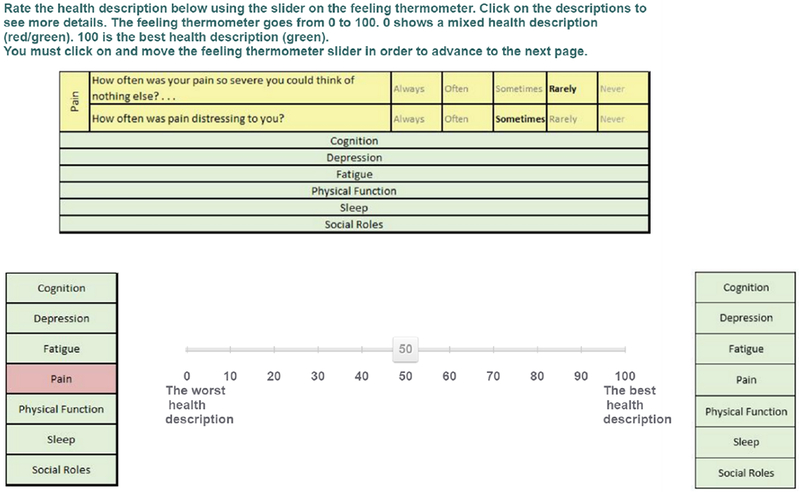
Participants valued the health states in two ways. The first was a warm-up exercise using a 0-100 visual analogue scale (VAS), sometimes called a Feeling Thermometer), where 0 is the value of a lower anchor state and 100 is the value of full health. An example appears in Figure B2 in the Appendix. This task was used to introduce the health states. The responses were used only in applying one exclusion criterion (violates-VAS), as explained below.
The second task used a standard gamble (SG) (25) to elicit utilities for the selected health states, a procedure that was pretested in the development of PROPr. The PROPr scoring system uses the SG method because of its grounding in expected utility theory (24,26). The specific SG task presented a health state and then offered a choice between (a) that state with certainty and (b) a lottery with probability p of full health and probability (1-p) of a lower anchor state. For single-domain valuation tasks, that lower anchor state had the worst level of functioning on that domain and the highest on all others; for multi-domain valuation tasks, the lower anchor was the all-worst state or dead (depending on which was worse for each participant, as indicated on earlier questions). Participants received a series of such choices, which varied p until they were indifferent between the lottery (b) and the certain option (a). The maximum for is thus 1, the utility of full health, and the minimum is 0, the utility of the lower anchor state. Figure B3 in the Appendix presents an example.
The PROPr online survey was completed by 1,164 participants selected to match the US 2010 Census as closely as possible for several demographic characteristics (see Table B2 in the Appendix for demographic information on the sample). The final sample was slightly older, more educated, with higher income and a greater proportion of White individuals than the overall US population. Excellent health was reported by 12.5%, very good health by 39.4%, good health by 33.8%, fair health by 12.4%, and poor health by 1.9%.
Exclusion Criteria
We selected 10 exclusion criteria representing the space defined by Table 1. Table 2 presents those 10 criteria. Some remove all responses (e.g., when participants do not pass a numeracy test threshold), whereas others only remove individual responses (e.g., those “trimmed” as too high or too low).
Table 2.
Core exclusion criteria. Core exclusion criteria, implemented with the PROPr data. Not every criterion from Table 1 is represented, because some would exclude no one by virtue of the design of the PROPr survey (e.g, there is no missing data). Unless otherwise indicated, valuations refer to the valuations of the single-domain states. Unshaded rows indicate preference-based criteria, shaded rows indicate process-based criteria.
Exclusion criteria (short-hand)
Requirements for exclusion
Violates dominance on the SG (violates-SG)
A participant, using the standard gamble (SG), violates dominance at least once.
Violates dominance on the VAS (violates-VAS)
A participant, using the visual analog scale (VAS), violates dominance at least once.
Valued the all-worst state or dead as the same or better than full health (dead-all-worst)
A participant is excluded if they rated the all-worst state or dead as the same or better than full health, using the standard gamble (SG).
Used less than 10% of the utility scale (low-range)
A participant is excluded if their valuations, using the standard gamble (SG), represent less than 10% of the range of the utility scale.
Provided the same response to every SG (no-variance)
A participant is excluded if they valued every state the same, using the standard gamble (SG).
In the top 5% of responses for an SG (upper-tail)
A response is excluded if it falls in the upper 5% of responses for that health state, using the standard gamble (SG).
In the bottom 5% of responses for an SG (lower-tail)
A response is excluded if it falls in the bottom 5% of responses for that health state, using the standard gamble (SG).
Score on the Subjective Numeracy Scale of less than 2.5 (numeracy)
A participant is excluded if they scored less than 2.5 on the short form of the Subjective Numeracy Scale (McNaughton, Cavanaugh, Kripalani, Rothman, & Wallston, 2015).
Self-assessed understanding equal to 1 or 2, on a scale of 1 = “Not at all” to 5 = “Very much” (understanding)
A participant is excluded if they rated themselves a “1” or a “2” on the self-assessed understanding question, which occurred after the preference elicitations.
15-minute time threshold (time)
A participant is excluded if they completed the PROPr survey in under 15 minutes.
We created this subset by (a) eliminating criteria not applicable in the PROPr data and (b) choosing the most stringent of “nested” criteria. Thus, we did not use “Valued too few health states” (Table 1, row 3) because the PROPr survey required participants to value all health states in the survey. “Nested” refers to criteria where exclusion by one necessarily implies exclusion by another – Table A1 in the Appendix shows examples of ways one might implement the criteria in Table 1 with the PROPr data, which include many nested examples. For example, some nested criteria differ in how many violations of dominance they tolerate before removing a participant. We used the most stringent of these criteria, which excludes even one such violation, designated violates-SG. We did, however, keep one pair of nested criteria: low-range and no-variance. Obviously, responses with no variance have a low range, meaning that no-variance is nested in low-range. However, no-variance has a unique relationship with violates-SG, in that someone excluded by one cannot also be excluded by the other, because giving the same utility for every health state (no variance) does not violate dominance. However, violating dominance means valuing two states differently (and in the “wrong” way), hence having variance. We also deviated from some researchers’ practice by having separate criteria for excluding the top 5% of responses (upper-tail) and the bottom 5% of responses (lower-tail), rather than combining them (10% trimming).
In our analyses of exclusion criteria, we treat each criterion as labeling each participant either for exclusion or inclusion, regardless of whether the criterion would exclude all or only some responses in an actual utility estimation analysis.
Multidimensional Scaling
Multidimensional scaling (MDS) provides a holistic picture of the similarities (and differences) between a set of objects (17), by translating pairwise comparisons among the objects into a graphical representation in which the distance between objects is a proxy for their similarity (16). Here, the objects are the exclusion criteria and the similarity metric assesses how well they agree about which participants to exclude. Each exclusion criterion is a binary classifier, either excluding or including each participant. The agreement of two binary classifiers can be represented in a confusion matrix like that in Table 3.
Table 3.
Confusion matrix. A confusion matrix (or 2-by-2 contingency table), which shows the possible outcomes of two joint binary variables (e.g., binary classifiers). We can consider each exclusion criteria as a classifier that categorizes a participant with a 1 if at least one of the participant’s responses would be excluded by the criterion, and a 0 otherwise. The table entries give the counts of the combinations of relationships: a is the number of participants excluded by both; b is the number excluded by criterion #1 that are included (not excluded) by criterion #2; c is the number excluded by criterion #2 that are included by criterion #1; and, d is the number included by both.
There are many possible summary indices for a confusion matrix (27–29). We chose one that incorporates each cell:
Known as the phi (ϕ) coefficient or the Matthews’ Correlation Coefficient (27,28,30,31), it is also the Pearson correlation for two binary variables. (The interpretation of phi differs somewhat from its continuous analog; for example, in how the distribution of each variable affects the possible values it can take.)
In the present application, given n exclusion criteria, the basic input to MDS is the n-by-n proximity matrix, denoted p, whose (i,j) entry pij is the phi value for the proximity of exclusion criteria i and j. The diagonal of the proximity matrix is 1 (i.e., pii = 1 for all i); the matrix is symmetric (i.e., pij = pji for all i and j), by construction.
When plotting the criteria, MDS uses the phi value of each pair of criteria and also considers the extent to which a pair identifies participants for exclusion in the same way as other criteria, by comparing their two rows of phi values in the proximity matrix, iterating over every pair. In doing so, MDS offers a visual display that demonstrates graphically the similarities and differences between criteria with respect to whom to exclude.
MDS algorithms produce m-dimensional configurations or plots, in which the distance between objects (here, the exclusion criteria) best approximate the values in the matrix (here, phi values), as measured by a goodness-of-fit (or stress) value. We used the ordinal algorithm because it makes the weakest assumptions about the data (29). For interpretability sake, we focus on m=2. Higher-dimensional configurations necessarily provide a better fit, but are more difficult to interpret (16). One of our sensitivity analyses adds a third dimension.
Structure in the MDS plot is seen in how the plotted objects cluster and align themselves dimensionally. In the present case, when criteria are close, it means that they exclude (and include) similar participants. The dimensions are not fixed, as the plot is equivalent under certain transformations, such as rotations. However, as with other procedures for reducing dimensionality (e.g., principal components analysis), there is no guarantee that any set of axes is interpretable.
We use the smacof package for the statistical software R (32) to identify the best-fit (lowest stress) solution, for placing the criteria consistently with the phi coefficients measuring the similarity of their exclusion patterns.
MDS sensitivity analysis
We performed the following sensitivity analyses:
a)
Dimensionality: We compared the 2-dimensional MDS solution with a 3-dimensional one. Adding dimensions necessarily improves the fit, but need not produce new interpretable structure. We compared the 2- and 3-dimensional solutions to see if the latter revealed new relationships.
b)
MDS jackknife: We repeated the analysis after removing each criterion (33), to see if any had disproportionate effect on the overall MDS solution.
c)
MDS algorithm: We compared the 2-dimensional MDS solution using the ordinal algorithm, with solutions produced using ratio, interval, and spline algorithms, in order to assess sensitivity to assumptions about the scale type of the input data.
d)
Clustering: We applied k-means clustering (34), to compare it with the graphical approach of MDS.
Section C2 of the Appendix reports the results of these sensitivity analyses, none of which produced materially different patterns.
Results
Table 4 shows how many PROPr participants are excluded by each criterion, which ranges from 7.8% (numeracy) to 84.7% (violates-VAS). Except for violates-VAS, the preference-based criteria are applied to participants’ SG valuations.
Table 4.
Number of participants flagged by each criterion. The number of participants in the PROPr data flagged by the each criterion from Table 2. The total number of participants in the sample is 1,164. Unshaded rows indicate preference-based criteria, shaded rows indicate process-based criteria.
Exclusion criterion
Number excluded (total sample n = 1164)
Violates dominance on the SG (violates-SG)
833 (71.6%)
Violates dominance on the VAS (violates-VAS)
986 (84.7%)
Valued the all-worst state or dead as the same or better than full health (dead-allworst)
326 (28.0%)
Provided the same response to every SG (no-variance)
137 (11.8%)
Used at less than 10% of the utility scale (low-range)
142 (12.2%)
In the top 5% of responses for an SG (upper-tail)
914 (78.5%)
In the bottom 5% of responses for an SG (lower-tail)
513 (44.1%)
Score on the Subjective Numeracy Scale of less than 2.5 (numeracy)
91 (7.8%)
Self-assessed understanding equal to 1 or 2, on a scale of 1 = “Not at all” to 5 = “Very much” (understanding)
Table 5 shows the matrix of phi values correlating the 10 exclusion criteria (Table 2). As phi is symmetric in its arguments, the correlation matrix in Table 4 is symmetric. The greatest agreement (0.98) is for (no-variance, low-range), the nested pair; the greatest disagreement (−0.58) is for (no-variance, violates-SG), the mutually exclusive pair. This matrix is the input to the MDS algorithm. (See the Appendix, section C1, for details.) As mentioned, similarity is forced with the two nested criteria, low-range and no-variance, which artifactually inflates goodness-of-fit for this solution.
Table 5.
Proximity matrix. The proximity matrix for the core criteria: each entry is the ϕ (phi) value of the exclusion criteria in the row and column. The shaded row and column titles indicate the process-based criteria, while the unshaded rows indicate the preference-based criteria
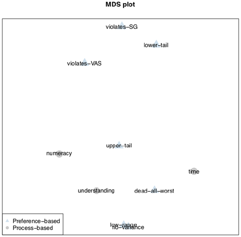
Figure 1 presents the 2-dimensional MDS plot of the exclusion criteria, with the distance between them showing how similarly they exclude participants. If exclusion criteria reflect similar mechanisms (e.g., inattention), they should be clustered closely.
The three process-based criteria have related rationales: (a) numeracy: low-numeracy participants may struggle to understand the demanding SG task; (b) time: participants who complete the survey quickly may not have made the effort needed to understand it; and (c) understanding: participants who report not understanding the task may have been confused or unusually self-critical. The relative proximity of these criteria in Figure 1 suggests that they reflect a common underlying process: inability or unwillingness to perform the SG task.
Preference-based criteria
The no-variance and low-range criteria are necessarily atop one another (at the center bottom of the figure), as they are nested, with identical responses (no-variance) being a special case of highly similar responses (low-range). Conversely, the most distant criteria in the figure are violates-SG and no-variance, which necessarily exclude different participants (as it is impossible to violate dominance when assigning the same value to all health states). The other relationships in the figure are empirical, rather than necessary ones.
Both violates-SG and violates-VAS are applied when participants rate a state with lower functional capacity or higher symptom burden as better than a state with higher functional capacity or lower symptom burden, thereby violating dominance. Both exclude many participants (Table 4). The fact that VAS excluded more may reflect its greater precision: The VAS allows increments of 0.01, whereas the SG only offers probability (hence utility) increments of 0.05. The two criteria lie close to one another in the MDS space, indicating that they exclude similar individuals.
Both, however, are far enough away from the process-based criteria (numeracy, understanding, time) that they appear to capture different mechanisms than those three measures of low-quality responses. Indeed, the fact that violates-SG is so distant suggests that it might remove some participants who are trying to express well-considered utilities but cannot do so without violating dominance. For example, some participants may prefer some depression to none, believing that it confers empathy that is valuable to their health. Similarly, some participants might prefer the worst possible cognitive ability to poor cognitive ability, when the former includes a lack of self-awareness, but the latter does not. Such preferences violate dominance deliberately. Other violations may include participants who have something to say but struggle with either the wording or the mechanics of the task. Researchers who use violates-SG as an exclusion criterion typically allow some violations, up to 11 in one study (1), suggesting that such struggles might be common. Box 1 describes one possible confusion pattern with the interface used here.
Box 1.
One possible account for high valuations is that the first question in the SG implementation presents a degenerate gamble where one option has a 100% probability of full health and 0% probability of the low anchor state (e.g., dead or the all-worst state), and the other option is the sure-thing of the intermediate state whose utility is being estimated. The participant can choose the gamble, the sure thing, or indifference. Choosing the gamble leads to a choice between a different gamble and the sure thing. Choosing the sure thing or expressing indifference completes the task and implies a utility estimate of 1 (or greater than 1 for those who select the sure thing). Therefore, making either of these last two choices leads to a response in the upper tail of the utility distribution. Thus, the mechanics of the procedure might lead to confused or inattentive responses being recorded as utilities in the upper tail of the response distribution, given that two of the three initial choices lead to an extreme utility value. Less numerate participants might be more likely to experience such confusion.
The dead-all-worst exclusion criterion represents a violation of dominance that arises when participants rate dead or the all-worst state as being at least as good as full health. Its proximity to time and understanding might indicate the kind of confusion that Box 1 suggests for violates-SG. However, the distance between dead-all-worst and violates-SG indicates different processes. Possibly participants who are excluded by violate-SG might be trying to express themselves but are frustrated by the interface design, whereas participants who violate dead-all-worst either cannot communicate their preferences or are not trying, leading them to say that they prefer dead or the all-worst state to full health. Doing so is an extreme violation of dominance, whereas violates-SG flags any violation, even among relatively similar health states.
The final two criteria, upper-tail and lower-tail remove the highest and lowest 5% of responses. (In our implementation, they flag anyone with a response eligible for such trimming.) Ten-percent trimming is a common practice, followed in constructing both the PROPr scoring system and the widely-used Health Utilities Index Mark 3 (21). The two criteria are far apart in Figure 1, indicating that they exclude different participants. Of the 513 flagged by lower-tail, 421 (82.1%) are flagged by upper-tail; conversely, lower-tail flags 57.0% of the 914 flagged by upper-tail. Phi reflects this asymmetry, with a value of 0.08 (Table 5) for the two criteria.
Both criteria apply to SG valuations for individual health states, and exclude based on how a participant’s response compares to those of other participants. However, as seen in Figure 1, the exclusion pattern for lower-tail is most similar to that for violates-SG, which compares a participant’s responses across health states, without consideration for how other participants respond. In contrast, the exclusion pattern for upper-tail is closest to those for numeracy and understanding, criteria that seem to exclude people who cannot or will not perform the task, which is more in line with the stated rationale of both trimming criteria. Thus, 10% trimming may remove two very different groups of participants: those who understand the task and explicitly express unusually low utilities and those who are confused by the task and inadvertently produce unusually high utilities.
Conclusion
Removing responses from datasets is a common practice in health utility studies (1) and other empirical research (35). Exclusion criteria formalize the removal process. Here, we analyze 10 exclusion criteria, chosen to represent those commonly used in health utility studies. We use multidimensional scaling (MDS) to compare their removal patterns, using the PROPr dataset as a testbed (22). Those criteria include preference-based ones, reflecting what participants said (e.g., unusually low utilities), and process-based ones, reflecting how they responded (e.g., unusually quickly).
The clustering of the three process-based criteria in Figure 1 suggests that they reflect related aspects of poor performance. In contrast, the spatial distribution of the preference-based criteria suggests that they reflect different mechanisms. As interpreted above, those mechanisms are sometimes at odds with the rationales given for using the criteria (Table 1). For example, upper-tail and lower-tail are far apart, despite commonly being combined using the same rationale (i.e., “aberrant” responses). Our analysis suggests that upper-tail responses reflect confusion or inattention, making them, in effect, preference-based reflections of response processes. In contrast, lower-tail responses appear to be deliberate expressions of low utilities. Thus, we propose that the two trimming criteria not be combined when the standard gamble is implemented in the same way as in PROPr (see Box 1). As a result, we analyze them separately in the companion article, which assesses the effects of applying these criteria on health state utility estimates.
These results and interpretations suggest ways in which future elicitation procedures might be improved, rendering fewer responses and participants as candidates for exclusion. Some investigators prefer in-person SG elicitations, such as the paper standard gamble (36), in order to reduce that task’s cognitive demands and any confusion caused by an unfamiliar computer interface. If online survey methods (37,38) are to achieve the potential benefits of low-cost data collection from demographically diverse samples, they need to reduce the cognitive demands of these tasks. One possible strategy is with interface designs that provide real-time feedback that helps users increase their understanding of the task without biasing their content. Those designs might include references to exclusion criteria, attention checks (39–42), or manipulation checks (43), asking whether participants understand the task, thereby communicating to the participant what the researcher expects from them (44). PROPr used in-person pilot testing to refine its survey design, as well as having participants complete the VAS to familiarize them with the health domain and consider their preferences for health, before completing the SG task. The approach demonstrated here and in the companion article, asking how preferences differ between the excluded and included, could be used to assess the impacts of competing designs. Those tests could be applied to other preference elicitation tasks as well, such as the time-tradeoff and discrete choice experiments (45,46).
None of the exclusion criteria considered here explicitly examine whether responses are informed (47), in the sense that preferences are based on considered reflection, possibly including personal experience of health states (e.g., through illness or care-giving). Choosing only informed preferences could be defined as an exclusion criterion, when there are measurements to operationalize it. Doing so requires analysts to consider the debate over whether health-related quality of life measurement should reflect the preferences of the general population or the people most directly involved (48).
Exclusion criteria pose a tradeoff between potentially improving data quality and potentially reducing sample representativeness. The present analyses provide insight into which responses different criteria remove and why. The companion paper analyzes their effects on estimates of health state utilities, complementing sensitivity analyses that re-analyze data with and without data exclusions. Its concluding section offers overall recommendations, drawing on the present results and those reported there. Both papers assume that exclusion criteria should be selected in advance, based on their rationale, and applied only if the data are consistent with that rationale. They offer complementary approaches to determining whether that is the case.
Acknowledgments
This research was completed at the Division of General Internal Medicine, the University of Pittsburgh, and the Department of Engineering & Public Policy, Carnegie Mellon University. Barry Dewitt received partial support from a Social Sciences and Humanities Research Council of Canada Doctoral Fellowship. Janel Hanmer was supported by the National Institutes of Health through Grant Number KL2 TR001856. Data collection was supported by the National Institutes of Health through Grant Number UL1TR000005. Baruch Fischhoff and Barry Dewitt were partially supported by the Swedish Foundation for the Humanities and Social Sciences. The funding agreements ensured the authors’ independence in designing the study, interpreting the data, writing, and publishing the report.
Appendix A. Exclusion criteria
Table A.1 provides additional examples of how exclusion criteria can be implemented in the PROPr dataset.
Table A.1: Examples of implementing exclusion criteria in PROPr.
Examples of how to implement the exclusion criteria from Table 1 in the main text of Exclusion I, using the PROPr data. Unless otherwise indicated, valuations refer to the valuations of the single-attribute states. Unshaded rows indicate preference-based criteria, shaded rows indicate process-based criteria.
Exclusion criterion
Requirements for exclusion
Violates dominance on the SG
A participant, using the standard gamble (SG), violates dominance at least once.
Violates dominance on the SG, more than twice
A participant, using the standard gamble (SG), violates dominance at least twice.
Violates dominance on the SG by more than 10% of the scale
A participant, using the standard gamble (SG), is considered to have violated dominance only if they do so by a difference of more than 0.1 on the utility scale.
Violates dominance on the SG by more than 10% of the scale, more than twice
A participant, using the standard gamble (SG), is considered to have violated dominance only if they do so by a difference of more than 0.1 on the utility scale, more than twice.
Violates dominance on the VAS
A participant, using the visual analog scale (VAS), violates dominance at least once.
Violates dominance on the VAS, more than twice
A participant, using the visual analog scale (VAS), violates dominance at least twice.
Violates dominance on the VAS by more than 10% of the scale
A participant, using the visual analog scale (VAS), is considered to have violated dominance only if they do so by a difference of more than 10 on the 0-100 VAS scale.
Violates dominance on the VAS by more than 10% of the scale, more than twice
A participant, using the standard gamble (SG), is considered to have violated dominance only if they do so by a difference of more than 10 on the 0-100 VAS scale.
Valued the all-worst state or dead as the same or better than full health.
A participant is excluded if they rated the all-worst state or dead as the same or better than full health, using the standard gamble (SG).
Used less than 10% of the utility scale
A participant is excluded if their valuations, using the standard gamble (SG), represent less than 10% of the range of the utility scale.
Provided the same response to every SG
A participant is excluded if they valued every state the same, using the standard gamble (SG).
In the top 5% of responses for an SG
A response is excluded if it falls in the top 5% of responses for that health state, using the standard gamble (SG).
In the bottom 5% of responses for an SG
A response is excluded if it falls in the bottom 5% of responses for that health state, using the standard gamble (SG).
Score on the Subjective Numeracy Scale of less than 2.5
A participant is excluded if they scored less than 2.5 on the short form of the Subjective Numeracy Scale (McNaughton, Cavanaugh, Kripalani, Rothman, & Wallston, 2015).
Self-assessed understanding equal to 1, on a scale of 1 = “Not at all” to 5 = “Very much”
A participant is excluded if they rated themselves a “1” on the self-assessed understanding question, which occurred after the preference elicitations.
Self-assessed understanding equal to 1 or 2, on a scale of 1 = “Not at all” to 5 = “Very much”
A participant is excluded if they rated themselves a “1” or a “2” on the self-assessed understanding question, which occurred after the preference elicitations.
15-minute time threshold
A participant is excluded if they completed the PROPr survey in under 15 minutes.
Figure B.1 shows the qualitative descriptors used to present health states to participants. Figure B.2 shows an example screen from the VAS elicitations. Figure B.3 shows an example screen from a standard gamble elicitation.
Table B.1 provides the theta scores corresponding to the health states valued by participants in the PROPr survey. Table B.2 provides demographic characteristics of the participants in the PROPr survey.
Qualitative descriptions of health states presented to survey participants. A single health state is represented by responses selected at every row. For single-domain health state utility elicitations, the other domains were kept at their highest levels.
An example valuation, using the standard gamble (SG).
Table B.1: PROMIS theta scores used in PROPr elicitation tasks.
The table shows the theta values corresponding to the health state descriptions valued in the PROPr survey. The levels between the unhealthiest and the healthiest correspond to the intermediate states valued in the elicitation task. The unhealthiest levels, together, define the all-worst state, while the best levels, together, define full health. The disutility corner state for a domain corresponds to the state described by the worst level on that domain, and the best on all others.
The first column shows the expected demographic characteristics based on the U.S. 2010 Census. The second column shows the demographic characteristics of the participants who completed the survey.
This section provides additional detail on MDS in general (section C.1) and the specific implementation in the manuscript (sections C.2 and C.3).
C.1. MDS implementations and goodness-of-fit
MDS takes a proximity matrix p – where each entry pij is the proximity between two objects – as input. An MDS algorithm then searches for a configuration X in m-dimensional space, such that the Euclidean distance in X between object i – an exclusion criterion, in our case – and object j, denoted by , is related to their proximity pij by some function f. This can be viewed as the problem of finding the configuration X, and the function f, such that the residual is minimized over all objects. More specifically, we seek to minimize the sum of squared eijs, which, when normed to account for the scale of X – recall that X is a geometric space, like a map, with arbitrary units of distance – is called stress [12].
The functional form of f defines the type of MDS, and depends on the scale type of the input data. For example, interval MDS – also known as classical MDS or metric MDS – assumes that the data is on at least an interval scale. That means the ratios of differences between proximities are meaningful, as they would be if the proximity index itself was Euclidean distance, as in our example of using MDS to recover the distances between cities. Interval MDS takes f to be a linear function of the proximities, i.e., f(pij) = a + bpij. In interval MDS, one minimizes stress by choosing different configurations and different parameters for f. Thus, finding an MDS solution is akin to performing linear regression to estimate f, while simultaneously adjusting the configuration of X, all in an attempt to find the lowest stress combination possible [12].
However, there are problems with interval MDS. Many proximity indices, including ϕ, are not on an interval scale [13]. Furthermore, although it is possible to transform indices to have interval-scale-like properties, doing so increases the number of assumptions one must make about the data: It requires that we trust the size of the differences between proximities just as much as we trust the proximities themselves. Allowing f to take on other functional forms provides more flexibility, requires making fewer assumptions about the data, and allows one to find better – i.e., lower stress – configurations.
One such alternative type of MDS is called ordinal (non-metric) MDS. Ordinal MDS uses ordinal regression, rather than linear regression, in the process of finding an optimal configuration X. Ordinal regression only tries to preserve the rank order of the proximity data. Thus, it only assumes that the arrangement of the objects (exclusion criteria) from least proximal to most proximal – however defined via a proximity index – is relatively stable. We use ordinal MDS because of its fewer assumptions.
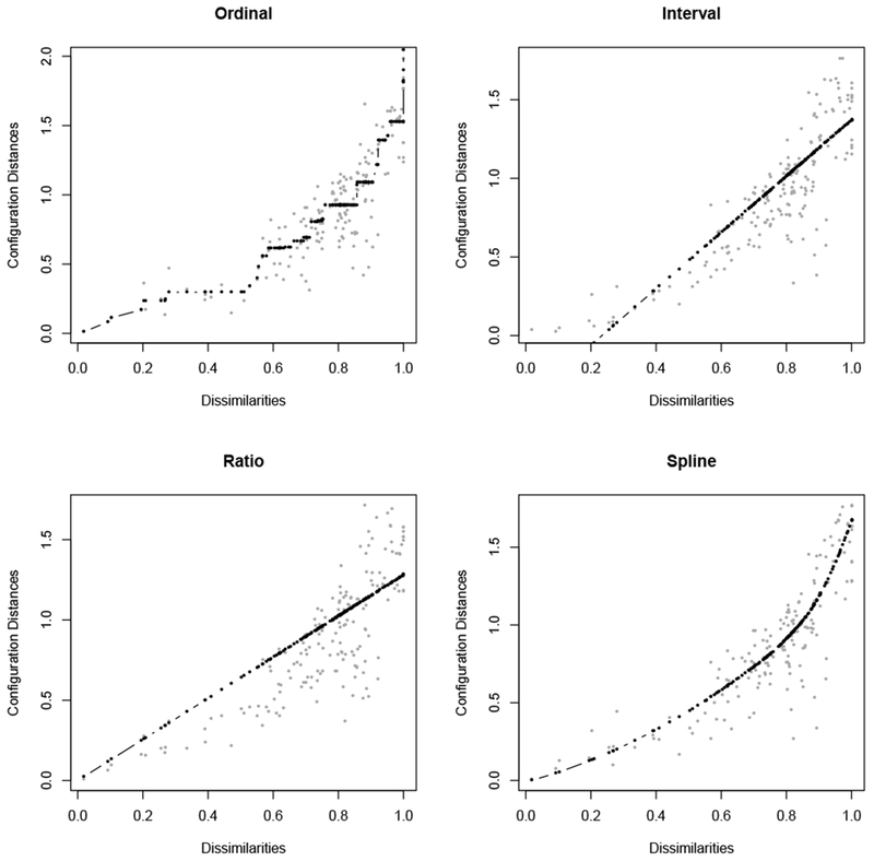
To see the difference between the types of MDS, Figure C.1 shows a Shepard plot for each. The Shepard plot displays the regression line of f. For technical reasons, the x-axis is not the proximity scale data, but a transformation of the proximities into dissimilarities, i.e., where 0 is the least dissimilar (most proximal) and positive numbers are increasingly dissimilar (less proximal).1 The y-axis shows the distances (the ) in the associated configuration. The points on the plot show how the dissimilarities are mapped to distances in the configuration. A good solution has small residuals. Note that a solution where every fitted value f(pij) coincided with its is not necessarily ideal, even though it obviously minimizes stress, because it is likely overfitting the data, just as in a regression with too much curvature. Rather, we look for a spread of the distances around the fitted values, such that we are not systematically violating the structure of the proximity data (e.g., the order of the distances roughly match the order of the distances), and the residuals do not show a systematic difficulty of scaling a particular size of dissimilarity.
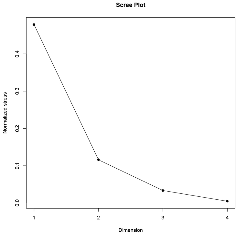
Another choice to make in the implementation of MDS is the dimensionality of the configuration space. The larger the number of dimensions, the better the fit of the scaling (in terms of stress), because there is more freedom to arrange the objects in the space. However, dimensions beyond three are difficult to use; even a 3-dimensional scaling of a few number of objects can be difficult to interpret. There is no definitive rule for choosing the number of dimensions. By convention, researchers rely on the change in stress combined with content knowledge of the application. Examining the Scree plot, which has the number of dimensions on the x-axis and the stress of a scaling of given dimensionality on the y-axis, can help with this process. The “elbow” of the plot, the step at which the change in stress diminishes visibly from the previous step, is taken as suggesting that one might be starting to scale the noise in the data. Figure C.2 shows an example.
A complementary approach starts with a 1-dimensional scaling, and adds dimensions, examining the resulting
Example Shepard plots from scalings using different MDS algorithms. The x-axis shows the dissimilarities – a transformation of the proximities – and the y-axis shows the distances between objects in the associated configuration. Each point is the distance between two objects, so there are points for n objects. The type of MDS algorithm – ordinal, interval, ratio, spline – determines the type of scale-type assumed for the dissimilarity and proximity data, and the type of regression used to minimize the residuals (the stress).
The x-axis shows the dimension of the MDS solution, and the y-axis shows the stress of that solution. By definition, stress decreases as the dimensionality increases, because there are more ways to scale the objects and maintain the relationships of the proximities. The “elbow” of the plot is the point at which the marginal decrease in stress changes abruptly, which is usually assumed to point to the best dimensionality for the MDS configuration. Here, that elbow is at 2-dimensions.
analyses for new structural relationships. When those cease, nothing is gained scientifically by increasing the dimensionality of the solution, even if, formally, the stress decreases. As the entire purpose of MDS is to gain insight on the structure of the objects by simultaneously representing all proximity relationships in a low-dimensional geometric configuration, then the lowest-dimensional useful representation can be “optimal,” in the sense that it avoids potentially scaling noise [14].
C.2. Results of the MDS sensitivity analysis and model-checking
Figure C.3 shows the Shepard plot for the main MDS plot (Figure 1 in the main text). It shows a good fit, with no systematic relationship to the residuals. There are other plots that provide useful diagnostics for evaluating the fit of an MDS solution, which are derived from the Shepard plot. Figure C.4 shows the stress-per-point. Recall that every point on the Shepard plot shows the relationship between one pair of criteria in terms of their proximity (as measured by ϕ) and its distance in the configuration. Each object in a scaling of n objects is associated with n−1 points in the Shepard plot. One can apportion the stress in the Shepard plot to each of the objects, by taking the sum of all the squared residuals involving that object and dividing by the total sum of squared residuals. Combining the stress-per-point plot for our core criteria (Figure C.4) with the main MDS plot, one can produce a configuration where each object is represented by a point whose size indicates the amount of stress associated with the scaling (Figure C.5). This is called a bubble plot. The larger the bubble, the more difficult it is for the MDS solution to scale that criterion. Figure C.4 and Figure C.5 show that low-range, no-variance, violates-VAS, and time were relatively easy to configure in 2-dimensional space, lower-tail, dead-all-worst, upper-tail, and numeracy were moderately easy, and placing understanding in the configuration was the most difficult aspect of scaling the 10 criteria. 2
Figure C.6 shows the Scree plot for ordinal MDS for the core criteria, with one, two, three, and four dimensions. The elbow appears at two dimensions. Thus, our primary scaling for the core criteria is a 2-dimensional MDS solution.
The results of other tests of our MDS model include the following:
a)
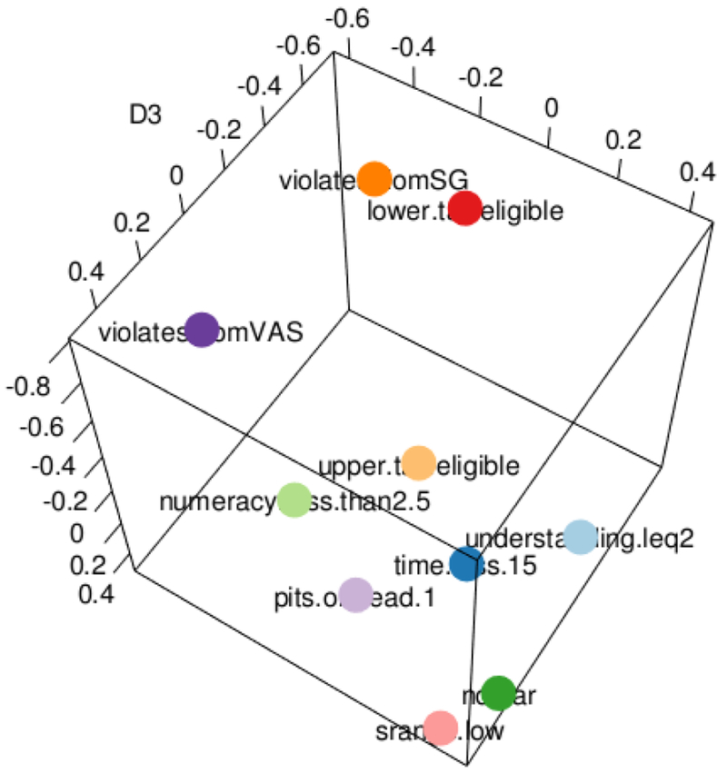
Dimensionality: Figure C.7 shows the 3-dimensional solution. It necessarily has a better fit than the 2-D solution, but at the risk of scaling noise. The relationships are similar to the 2-dimensional configuration, but the five difficult-to-scale criteria are separated from the others along the third dimension – lowering the stress of the configuration. The pairwise distances of the 3-dimensional configuration and the 2-dimensional configuration have a linear correlation of 0.93 (p-value < 0.01).
b)
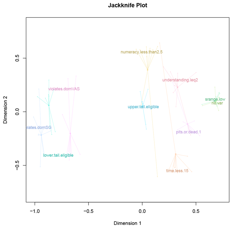
MDS jackknife: Figure C.8 shows an MDS jackknife plot, demonstrating how each criterion moves when one of the other criteria are removed from the MDS and the configuration is re-calculated. We can use those
Figure C.3: Shepard plot for core MDS configuration.
The stress-per-point plot calculates all of the squared residuals from the Shepard plot (Figure C.3), and apportions those residuals (the stress) among the criteria. Those with larger proportions of stress were more difficult to scale; i.e., it is more difficult to maintain all of the proximity relationships of that criterion when producing the configuration.
The bubble-plot of the core MDS solution combines the core MDS plot and Figure C.4, showing the configuration with each object represented by a bubble demonstrating the stress apportioned to that criterion. The larger the bubble, the more difficult it was to scale that criterion.
The scree plot for ordinal MDS solutions of the core criteria, with the elbow at 2-dimensions.
changes to calculate a dispersion statistic, which measures the average difference between the “leave-one-out” solutions and the original solution. It has a maximum of 2 – meaning that the original solution is highly sensitive to the inclusion of each object – and a minimum of 0 (low dispersion). The dispersion value for the core solution is 0.19.
c)
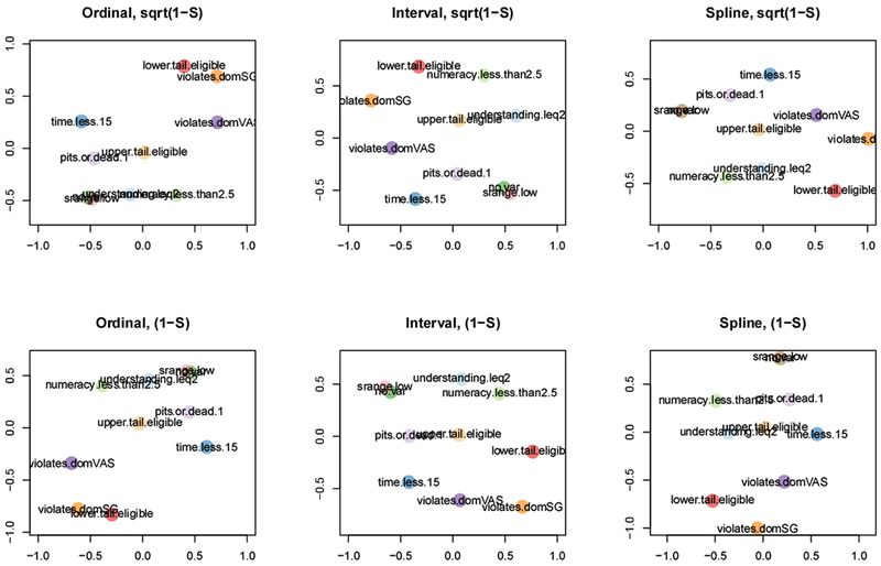
MDS algorithm: Other MDS models are possible, including interval and spline MDS, shown in (Figure C.9). The spline is most similar to the ordinal MDS solution in the main text. They are shown alongside a different transformation of the ϕ proximity index into a dissimilarity index.
d)
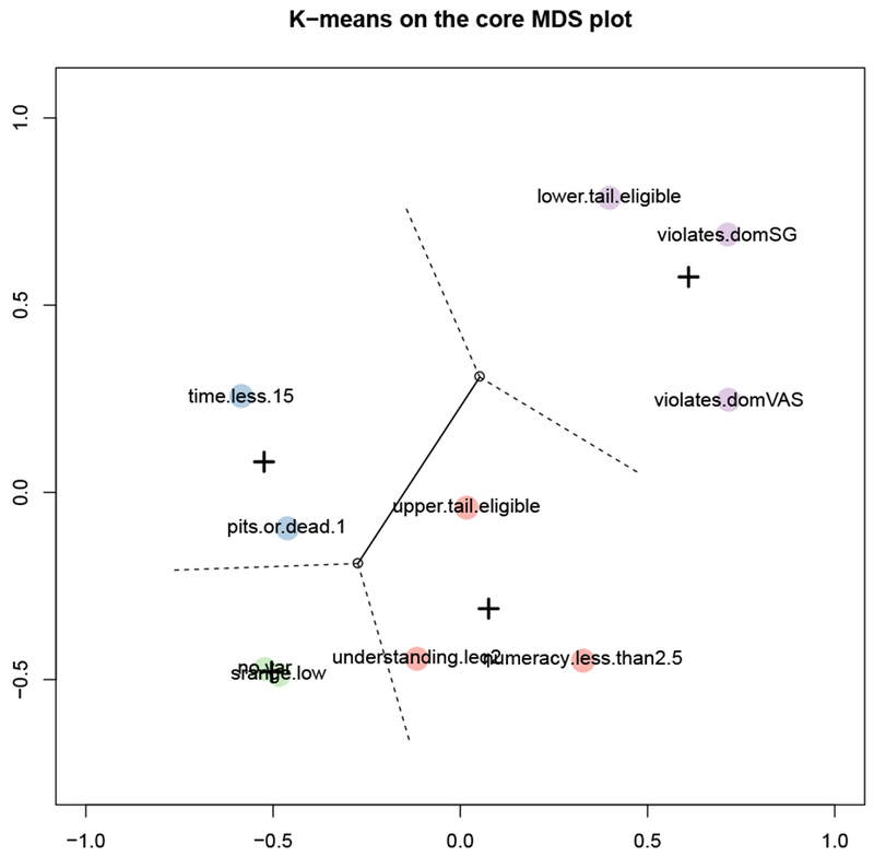
Clustering: In a k-means clustering analysis, we choose k in order to minimize within-cluster variance, and use a Scree plot to find the k at which adding another cluster is not uncovering more group structure in the data, by looking for a decrease in the improvement of within-cluster variance. (After all, when k equals the number of objects, within-cluster variance is 0 – but we learn nothing about the potential group structure.) Using k-means provides a computational approach to observing structure in the MDS plot, to compare with our own observations. Figure C.10 shows the configuration with a clustering with k = 4, the optimal k for this configuration. It places violation-SG, violation-VAS, and lower-tail in one group; upper-tail, numeracy, and understanding in a second group; time in a third dead-all-worst; and, no-variance and low-range in a fourth.
C.3. Discussion of the MDS sensitivity analysis
a)
Dimensionality: We cannot see any new structure in the 3-dimensional configuration that is not already present in the 2-dimensional configuration, except a difference in the order of dead-all-worst, time, and understanding. The third dimension does not seem interpretable in-and-of itself. That gives us confidence that two dimensions provides a useful solution.
b)
MDS jackknife: The jackknife solution and dispersion statistic show that large patterns are robust (e.g., the placement of violates-SG, violates-VAS, and lower-tail). The individual placement of criteria in the space can vary depending on which criterion is left out of the scaling, with the biggest changes along the vertical dimension of Figure C.8. That means the relationships along that dimension are highly influenced by the exact set of criteria – but none of the alternative scaling produced by removing a single criterion would produce a drastically different interpretation. It also means that the criteria capture a variety of mechanisms (except for the low-range and no-variance pair). Otherwise, the redundancy of including them would show itself in the jackknife diagram, where removing a criterion would not have much of an influence on the placements of the others.
c)
MDS algorithm: The transformation of ϕ appears to make less of a difference than the algorithm type; while the ordinal and spline algorithms produce similar results, the interval algorithm produces a different configuration. The assumptions made of the data are strongest in interval and weakest in ordinal MDS. That the configuration is similar with the spline is one mark for the robustness of the core solution. That the configuration is different with the interval MDS means that treating (a transformation of) ϕ as interval-scaled could produce different conclusions. Interval MDS requires maintaining the differences between the dissimilarities. Those differences are hard to interpret, even among small numbers of criteria, and hence we have not prioritized interpreting them.
d)
Clustering: The k-means clustering does not provide us with any additional information: the groupings do not lead to new conclusions that are not readily available from the configuration without the clustering.
Figure C.7: 3-dimensional MDS configuration for core criteria.
A view of the 3-dimensional configuration corresponding to 3-dimensional ordinal MDS using the core criteria. Notice the similarity of this view to core MDS plot in the main text.
Figure C.8: Jackknife plot for core configuration.
A jackknife plot corresponding to the main MDS plot, showing how each criterion moves when one of the others are removed and the MDS is re-computed. The labels show the original configuration, and the centre points the centroid of all of the leave-one-out MDS solutions.
Figure C.9: MDS using different algorithms and transformations of ϕ.
Each panel of this figure shows the MDS configuration using one of ordinal, interval, or spline MDS, and either the 1 − ϕ or transformation of phi into an index of dissimilarity. The leftmost column shows two identical plots (by denition), equivalent to the main MDS plot.
The main MDS plot, with a colouring of the criteria demonstrating the solution to k-means clustering with k = 4. The crosses indicate the centroids of the clusters, and the empty dot the centroid of the entire configuration. K-means is a computational search for structure in the configuration, analogous to the researcher using his or her own eyes to see patterns in the configuration.
Footnotes
1
In order to turn the ϕ index into an index of dissimilarity, there are two possible transformations: 1 − ϕ or [13]. They have the same ordinal properties, but can change the results of the other MDS algorithms.
2
Note that these figures, as well as some others in the Appendix, use the variable names for the exclusion criteria in our data set, rather than the shorthands in the main text. The mapping from one to the other should be clear.
Contributor Information
Barry Dewitt, Department of Engineering & Public Policy, Carnegie Mellon University, Pittsburgh, PA.
Baruch Fischhoff, Department of Engineering & Public Policy and the Institute for Politics and Strategy, Carnegie Mellon University, Pittsburgh, PA.
Alexander L. Davis, Department of Engineering & Public Policy, Carnegie Mellon University, Pittsburgh, PA.
Stephen B. Broomell, Department of Social and Decision Sciences, Carnegie Mellon University, Pittsburgh, PA.
Mark Roberts, Department of General Internal Medicine, University of Pittsburgh Medical Center, Pittsburgh, PA and Department of Health Policy and Management, University of Pittsburgh, Pittsburgh, PA.
Janel Hanmer, Department of General Internal Medicine, University of Pittsburgh Medical Center, Pittsburgh, PA.
References
1.Engel L, Bansback N, Bryan S, Doyle-Waters MM, Whitehurst DGT. Exclusion Criteria in National Health State Valuation Studies: A Systematic Review. Med Decis Mak [Internet]. 2016;36(7):798–810. Available from: http://www.ncbi.nlm.nih.gov/pubmed/26209475 [DOI] [PubMed] [Google Scholar]
2.Wilson IB, Cleary PD. Linking clinical variables with health-related quality of life: A conceptual model of patient outcomes. JAMA. 1995;273(1):59–65. [PubMed] [Google Scholar]
3.Neumann PJ, Goldie SJ, Weinstein MC. Preference-Based Measures in Economic Evaluation in Health Care. Annu Rev Public Heal. 2000;21:587–611. [DOI] [PubMed] [Google Scholar]
5.Broeck J Van Den, Cunningham SA, Eeckels R, Herbst K. Data Cleaning: Detecting, Diagnosing, and Editing Data Abnormalities. PLoS Med. 2005;2(10). [DOI] [PMC free article] [PubMed] [Google Scholar]
6.Boyd D, Crawford K. Critical Question for Big Data: Provocations for a cultural, technological, and scholarly phenomenon. Information, Commun Soc. 2012;15(5):662–79. [Google Scholar]
7.Devlin NJ, Hansen P, Kind P, Williams A. Logical inconsistencies in survey respondents’ health state valuations - A methodological challenge for estimating social tariffs. Health Econ. 2003;12(7):529–44. [DOI] [PubMed] [Google Scholar]
8.Devlin NJ, Hansen P, Selai C. Understanding health state valuations: A qualitative analysis of respondents’ comments. Qual Life Res. 2004;13(7):1265–77. [DOI] [PubMed] [Google Scholar]
9.Lancsar E, Louviere J. Deleting “irrational” responses from discrete choice experiments: A case of investigating or imposing preferences?
Health Econ. 2006;15(8):797–811. [DOI] [PubMed] [Google Scholar]
10.Lamers LM, Stalmeier PFM, Krabbe PFM, Busschbach JJV. Inconsistences in TTO and VAS Values for EQ-5D Health States. Med Decis Mak. 2006;26(2):173–81. [DOI] [PubMed] [Google Scholar]
11.Fischhoff B, Kadvany J. Risk: A Very Short Introduction. New York: Oxford University Press; 2011. [Google Scholar]
13.Edwards W
The Theory of Decision Making. Psychol Bull. 1954;51(4):380–417. [DOI] [PubMed] [Google Scholar]
14.Law EH, Pickard AL, Kaczynski A, Pickard AS. Choice Blindness and Health-State Choices among Adolescents and Adults. Med Decis Mak. 2017;37(6):680–7. [DOI] [PubMed] [Google Scholar]
15.Wittenberg E, Prosser LA. Ordering errors, objections and invariance in utility survey responses: A framework for understanding who, why and what to do. Appl Health Econ Health Policy. 2011;9(4):225–41. [DOI] [PubMed] [Google Scholar]
16.Borg I, Groenen PJF. Modern multidimensional scaling: Theory and applications. Springer; 2005. [Google Scholar]
17.Baird JC, Noma EJ. Fundamentals of Scaling and Psychophysics. John Wiley & Sons; 1978. [Google Scholar]
18.Shepard RN. Multidimensional scaling, tree-fitting, and clustering. Science. 1980. p. 390–8. [DOI] [PubMed] [Google Scholar]
19.Hanmer J, Dewitt B. PROMIS-Preference (PROPr) Score Construction -- A Technical Report [Internet]. 2017.
Available from: janelhanmer.pitt.edu/PROPr.html
21.Feeny D, Furlong W, Torrance GW, Goldsmith CH, Zhu Z, DePauw S, et al.
Multiattribute and single-attribute utility functions for the Health Utilities Index Mark 3 system. Med Care. 2002;40(2):113–28. [DOI] [PubMed] [Google Scholar]
23.Hanmer J, Cella D, Feeny D, Fischhoff B, Hays RD, Hess R, et al.
Selection of key health domains from PROMIS® for a generic preference-based scoring system. Qual Life Res. Springer International Publishing; 2017;1–9. [DOI] [PMC free article] [PubMed] [Google Scholar]
24.Keeney RL, Raiffa H. Decisions with multiple objectives: Preferences and value tradeoffs. New York, NY: John Wiley & Sons; 2003. [Google Scholar]
26.von Neumann J, Morgenstern O. Theory of games and economic behaviour. Princeton University Press; 1944. [Google Scholar]
27.Gower JC, Legendre P. Metric and Euclidean properties of dissimilarity coefficients. J Classif. 1986;3:5–48. [Google Scholar]
28.Warrens MJ. On association coefficients for 2 × 2 tables and properties that do not depend on the marginal distributions. Psychometrika. 2008;73(4):777–89. [DOI] [PMC free article] [PubMed] [Google Scholar]
29.Borg I, Groenen PJF, Mair P. Applied multidimensional scaling. Springer; 2012. [Google Scholar]
30.Matthews BW. Comparison of the predicted and observed secondary structure of T4 phage lysozyme. BBA - Protein Struct. 1975;405(2):442–51. [DOI] [PubMed] [Google Scholar]
31.Yule GU. On the methods of measuring the association between two attributes. J R Stat Soc. 1912;75(6):579–652. [Google Scholar]
32.de Leeuw J, Mair P. Multidimensional Scaling Using Majorization: SMACOF in R. J Stat Softw. 2009;31(3):1–30. [Google Scholar]
33.de Leeuw J, Meulman J. A special Jackknife for Multidimensional Scaling. J Classif. 1986;3(1):97–112. [Google Scholar]
34.Bishop CM. Pattern Recognition and Machine Learning. Springer; 2006. [Google Scholar]
36.Ross PL, Littenberg B, Fearn P, Scardino PT, Karakiewicz PI, Kattan MW. Paper standard gamble: A paper-based measure of standard gamble utility for current health. Int J Technol Assess Health Care. 2003;19(1):135–47. [DOI] [PubMed] [Google Scholar]
37.Buhrmester M, Kwang T, Gosling SD. Amazon’s Mechanical Turk: A New Source of Inexpensive, Yet High-Quality, Data?
Perspect Psychol Sci. 2011;6(1):3–5. [DOI] [PubMed] [Google Scholar]
38.Leeuw ED De. Counting and Measuring Online: The Quality of Internet Surveys. Bull Méthodologie Sociol. 2012;68–78. [Google Scholar]
39.Hauser DJ, Schwarz N. Attentive Turkers: MTurk participants perform better on online attention checks than do subject pool participants. Behav Res Methods. 2016;48(1):400–7. [DOI] [PubMed] [Google Scholar]
41.Abbey JD, Meloy MG. Attention by design: Using attention checks to detect inattentive respondents and improve data quality. J Oper Manag [Internet]. Elsevier Ltd; 2017;53–56:63–70. Available from: 10.1016/j.jom.2017.06.001 [DOI] [Google Scholar]
42.Peer E, Vosgerau J, Acquisti A. Reputation as a sufficient condition for data quality on Amazon Mechanical Turk. Behav Res Methods. 2014;46(4): 1023–31. [DOI] [PubMed] [Google Scholar]
43.Oppenheimer DM, Meyvis T, Davidenko N. Instructional manipulation checks: Detecting satisficing to increase statistical power. J Exp Soc Psychol [Internet], Elsevier Inc.; 2009.
July
[cited 2014 Jul 12];45(4):867–72. Available from: http://linkinghub.elsevier.com/retrieve/pii/S0022103109000766 [Google Scholar]
45.Weinstein MC, Torrance G, Mcguire A. QALYs: The Basics. Value Heal [Internet]. International Society for Pharmacoeconomics and Outcomes Research (ISPOR); 2009;12:S5–9. Available from: 10.1111/j.1524-4733.2009.00515.x [DOI] [PubMed] [Google Scholar]
46.Ratcliffe J, Brazier J, Tsuchiya AKI, Symonds T, Brown M. Using DCE and Ranking Data to Estimate Cardinal Values for Health States for Deriving a Preference-Based Single Index from the Sexual Qualifty of Life Questionnaire. Health Econ. 2009;18:1261–76. [DOI] [PubMed] [Google Scholar]
47.Karimi M, Brazier J, Paisley S. Are preferences over health states informed? Health Qual Life Outcomes. Health and Quality of Life Outcomes; 2017;15(1):1–11. [DOI] [PMC free article] [PubMed] [Google Scholar]
48.Versteegh MM, Brouwer WBF. Patient and general public preferences for health states: A call to reconsider current guidelines. Soc Sci Med [Internet], Elsevier Ltd; 2016;165:66–74. Available from: 10.1016/j.socscimed.2016.07.043 [DOI] [PubMed] [Google Scholar]
Bibliography
[1].Hays RD, Spritzer KL, Thompson WW and Cella D, U.S. General Population Estimate for “Excellent” to “Poor” Self-Rated Health Item, J Gen Intern Med, Vol. 30, No. 10, pp. 1511–1516, 2015.
7 [DOI] [PMC free article] [PubMed] [Google Scholar]
[2].Hays RD, Bjorner J, Revicki DA, Spritzer KL and Cella D, Development of physical and mental health summary scores from the Patient-Reported Outcomes Measurement Information System (PROMIS) global items., Quality of Life Research, Vol. 18, 2009.
7 [DOI] [PMC free article] [PubMed] [Google Scholar]
[3].Herdman M, Gudex C, Lloyd A, Janssen M, Kind P, Parkin D, Bonsel G and Badia X, Development and preliminary testing of the new five-level version of EQ-5D (EQ-5D-5L), Quality of Life Research, Vol. 20, No. 10, pp. 1727–1736, 2011.
7 [DOI] [PMC free article] [PubMed] [Google Scholar]
[4].Feeny D, Furlong W, Torrance GW, Goldsmith CH, Zhu Z, DePauw S, Denton M and Boyle M, Multiattribute and Single-Attribute Utility Functions for the Health Utilities Index Mark 3 System, Medical Care, Vol. 40, No. 2, pp. 113–128, 2002.
7 [DOI] [PubMed] [Google Scholar]
[5].Torrance GW, Feeny D, Furlong WJ, Barr RD, Zhang Y and Wang Q, Multiattribute utility function for a comprehensive health status classification system: Health Utilities Index Mark 2, Medical Care, Vol. 34, No. 7, pp. 702–722, 1996.
7 [DOI] [PubMed] [Google Scholar]
[6].CDC, Chronic Disease Overview, 2016.
7
[7].Gershon RC, Rothrock N, Hanrahan R, Bass M and Cella D, The use of PROMIS and Assessment Center to deliver Patient-Reported Outcome Measures in clinical research, Journal of Applied Measurement, Vol. 11, No. 3, pp. 304–314, 2010.
7 [PMC free article] [PubMed] [Google Scholar]
[9].Fagerlin A, Zikmund-Fisher BJ, Ubel PA, Jankovic A, Derry HA and Smith DM, Measuring numeracy without a math test: Development of the Subjective Numeracy Scale., Medical Decision Making, Vol. 27, No. 5, pp. 672–80, 2007.
7 [DOI] [PubMed] [Google Scholar]
[10].McNaughton CD, Cavanaugh KL, Kripalani S, Rothman RL and Wallston KA, Vali-dation of a Short, 3-Item Version of the Subjective Numeracy Scale, Medical Decision Making, Vol. 35, No. 8, pp. 932–936, 2015.
7 [DOI] [PMC free article] [PubMed] [Google Scholar]
[11].Hanmer J and Dewitt B, PROMIS-Preference (PROPr) Score Construction – A Technical Report. 7
[12].Borg I and Groenen PJF, Modern multidimensional scaling: Theory and applications, Springer, 2005.
13 [Google Scholar]
[13].Gower JC and Legendre P, Metric and Euclidean properties of dissimilarity coefficients, Journal of Classification, Vol. 3, pp. 5–48, 1986.
13, 14 [Google Scholar]
[14].Borg I, Groenen PJF and Mair P, Applied multidimensional scaling, Springer, 2012.
17 [Google Scholar]


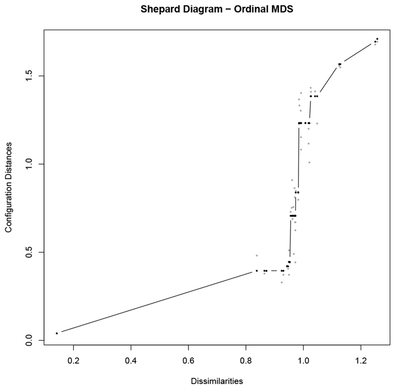 The Shepard plot for the core MDS solution, using the ordinal MDS algorithm.
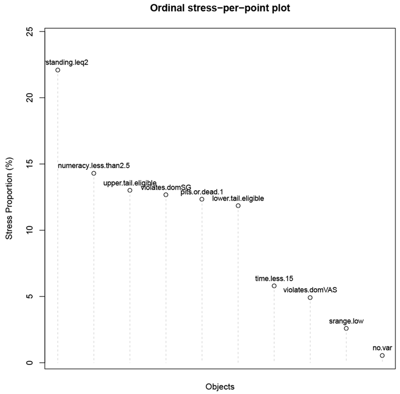 The stress-per-point plot calculates all of the squared residuals from the Shepard plot (Figure C.3), and apportions those residuals (the stress) among the criteria. Those with larger proportions of stress were more difficult to scale; i.e., it is more difficult to maintain all of the proximity relationships of that criterion when producing the configuration.
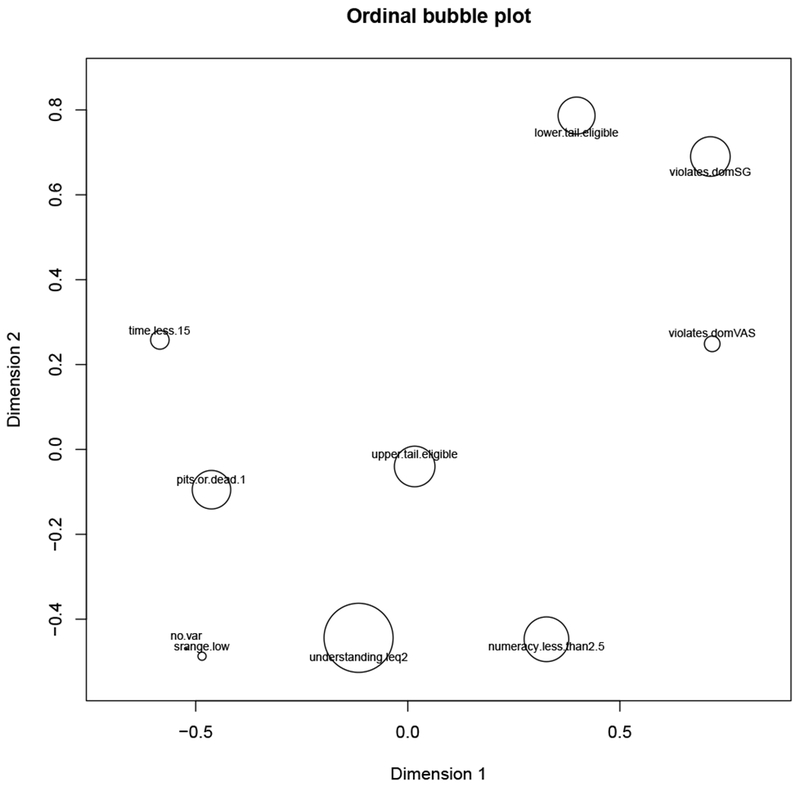 The bubble-plot of the core MDS solution combines the core MDS plot and Figure C.4, showing the configuration with each object represented by a bubble demonstrating the stress apportioned to that criterion. The larger the bubble, the more difficult it was to scale that criterion.
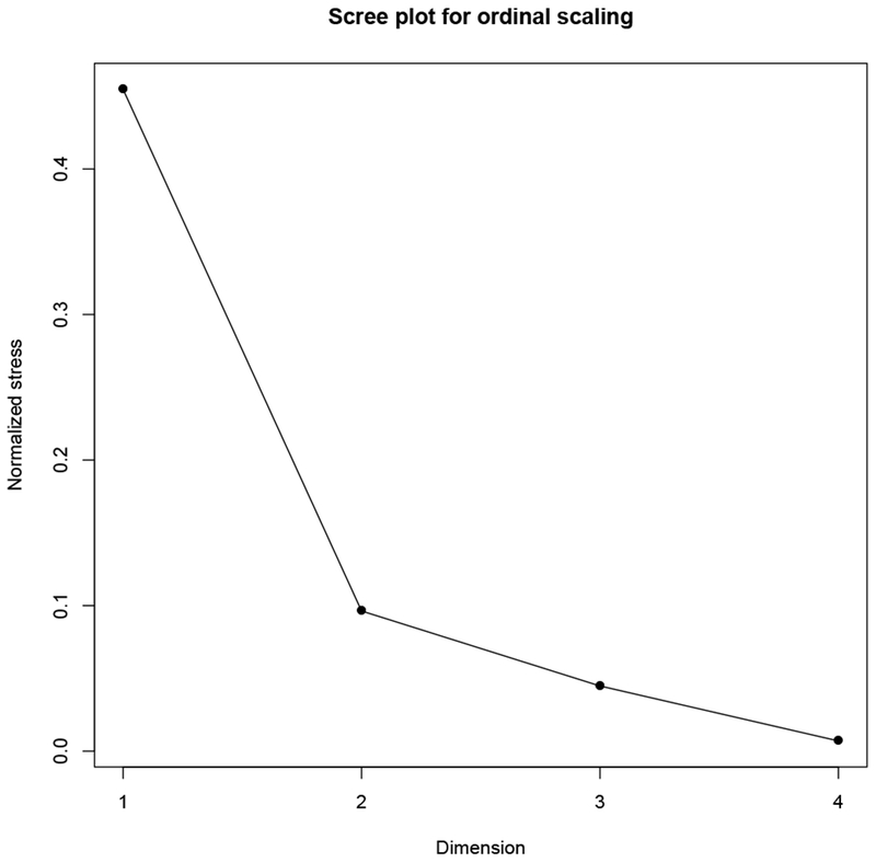 The scree plot for ordinal MDS solutions of the core criteria, with the elbow at 2-dimensions.