

Abstract
Background:
Researchers often justify excluding some responses in studies eliciting valuations of health states as not representing respondents’ true preferences. Here, we examine the effects of applying 8 common exclusion criteria on societal utility estimates.
Setting:
An online survey of a U.S. nationally representative sample (n=1164) used the standard gamble method to elicit preferences for health states defined by 7 health domains from the Patient-Reported Outcomes Measurement Information System (PROMIS®).
Methods:
We estimate the impacts of applying 8 commonly used exclusion criteria on mean utility values for each domain, using beta regression, a form of analysis suited to double-bounded scales like utility.
Results:
Exclusion criteria have varied effects on the utility functions for the different PROMIS health domains. As a result, applying those criteria would have varied effects on the value of treatments (and side effects) that change health status on those domains.
Limitations:
Although our method could be applied to any health utility judgments, the present estimates reflect the features of the study that produced them. Those features include the selected health domains, standard-gamble method, and online format that excluded some groups (e.g., visually impaired and illiterate individuals). We also examined only a subset of all possible exclusion criteria, selected to represent the space of possibilities, as characterized in a companion article.
Conclusions:
Exclusion criteria can affect estimates of the societal utility of health states. We use those effects, in conjunction with the results of a companion article, to make suggestions for selecting exclusion criteria in future studies.
Introduction
Utility-based measures of health-related quality of life provide quantitative estimates of preferences for health states, and are commonly used in cost-effectiveness and cost-utility analyses, decision analyses, clinical trials, and population health studies (1). Here, we address a problem that the creators of such measures often face: applying exclusion criteria to remove responses that appear not to reflect true preferences, a process that Engel and colleagues (2) have shown can often remove a substantial proportion of the collected data, sometimes more than half. A companion article examines 10 common exclusion criteria in terms of how and why they agree and disagree about which responses to treat as unacceptable (3). Here, we consider the effects of applying 8 of these criteria on mean societal valuations of health states. We propose a general method, illustrated with utility data for one widely-used set of health-state measures, the Patient-Reported Outcomes Measurement Information System® (PROMIS®).
PROMIS, an initiative of the National Institutes of Health, offers psychometrically constructed scales for eliciting self-reported health states on many domains (4). The PROMIS-Preference (PROPr) scoring system (5) creates societal utility scores for 7 PROMIS domains: Cognitive Function - Abilities (cognition); Emotional Distress – Depression (depression); Fatigue (fatigue); Pain – Interference (pain); Physical Function (physical function); Sleep Disturbance (sleep); and Ability to Participate in Social Roles and Activities (social roles). PROPr also offers a multi-attribute utility function (6) for estimating a single health utility score from these 7 domains. Following convention (7–9), those utilities reflect the responses of representative samples of the general public to questions using the standard gamble method.
Two features of single-domain utility functions determine their impact on health policy analyses: their elevation (absolute value), showing how much intermediate health states are valued relative to the worst and full health states, and their sensitivity (curvature), showing how utility changes with changes in health status. Exclusion criteria that increase elevation potentially reduce the value of interventions designed to a improve a given health state and the aversiveness of side effects that degrade it. Exclusion criteria that reduce the elevation could do the opposite. Exclusion criteria that increase the curvature of a health utility curve increase the value of treatment that move people to better health states and the aversiveness of side effects that move people to poorer states. Exclusion criteria that result in flatter curves do the opposite.
We focus on single-domain utility functions because they are the input data used to calculate multi-attribute utility scores. PROPr’s multi-attribute scoring system for its 7 domains applies some of the exclusion criteria studied below – the removal of extreme responses and the responses of those who completed its associated data collection survey in under 15 minutes. Dewitt et al. (5) analyze the effects of several exclusion choices on the multi-attribute score. That sensitivity analysis complements the analysis here, which reveals the effects of exclusion on mean utility estimates without the extra structure required to produce the multi-attribute score, in terms that are meaningful to those who might use them (i.e., that of cost-effectiveness). That structure can obscure the effects of exclusion criteria on the included preferences, by requiring, for example, single-domain functions to go through 0 and 1 at prescribed points. Focusing on the single-domain functions allows us to see the variety of effects with different combinations of health domains and exclusion criteria.
The next section introduces the 8 exclusion criteria and the PROPr survey. We then explain the modeling approach, beta regression, apply it to the PROPr survey responses, discuss policy implications, and offer recommendations for evaluating exclusion criteria.
Methods
Data
Our analyses use data from the PROMIS-Preference (PROPr) Scoring System survey, described more fully in (5,11–13), the companion article (3), and Section A in the Appendix. Briefly, 1,164 participants were sampled to be representative demographically of the U.S. general population. They evaluated health states on one of 7 PROMIS health domains. The visual analog scale (VAS) was first used to familiarize them with the domains and was followed by the standard gamble (SG), which was used to estimate the PROPr health state utilities, given its normative properties (14). We focus on those SG responses here. Participants were randomly selected to evaluate one of the 7 health domains. Depression and social roles were evaluated by 167 participants; the other domains by 166. Participants also evaluated other health states, such as dead or the all-worst state. They answered several other tasks as well, described in the other sources.
Exclusion criteria
Exclusion criteria seek to distinguish true preferences from confused, inattentive, or strategic (deliberately biased) ones. Criteria can be preference-based, reflecting a respondent’s choices (e.g., unusually high values), or process-based, reflecting how respondents produced them (e.g., too quickly to be thoughtful).
Table 1 shows 10 criteria, selected to represent the space of commonly invoked rationales, including both preference-based and process-based ones – Section B in the Appendix shows more examples. The companion article (3) applies multi-dimensional scaling (MDS) to characterize these criteria in terms of how similarly they select participants for exclusion. Two criteria, low-range and no-variance, are nested, in the sense that they apply the same rule, one more stringently than the other. Here, we just use low-range, which subsumes no-variance. We exclude one criterion (violates-VAS) that does not apply to the standard gamble, but which might be examined with the present analytical framework in a comparison of the two elicitation procedures.
Table 1.
Core exclusion criteria. Core exclusion criteria, implemented with the PROPr data. Unless otherwise indicated, valuations refer to the valuations of the single-domain states. Unshaded rows indicate preference-based criteria, shaded rows indicate process-based criteria.
| Exclusion criteria (short-hand) | Requirements for exclusion |
|---|---|
| Violates dominance on the SG (violates-SG) | A participant, using the standard gamble (SG), violates dominance at least once. |
| Violates dominance on the VAS (violates- VAS) | A participant, using the visual analog scale (VAS), violates dominance at least once. |
| Valued the all-worst state or dead as the same or better than full health (dead-all-worst) | A participant is excluded if they rated the all-worst state or dead as the same or better than full health, using the standard gamble (SG). |
| Used less than 10% of the utility scale (low-range) | A participant is excluded if their valuations, using the standard gamble (SG), represent less than 10% of the range of the utility scale. |
| Provided the same response to every SG (no-variance) | A participant is excluded if they valued every state the same, using the standard gamble (SG). |
| In the top 5% of responses for an SG (upper-tail) | A response is excluded if it falls in the upper 5% of responses for that health state, using the standard gamble (SG). |
| In the bottom 5% of responses for an SG (lower-tail) | A response is excluded if it falls in the bottom 5% of responses for that health state, using the standard gamble (SG). |
| Score on the Subjective Numeracy Scale of less than 2.5 (numeracy) | A participant is excluded if they scored less than 2.5 on the short form of the Subjective Numeracy Scale (McNaughton, Cavanaugh, Kripalani, Rothman, & Wallston, 2015). |
| Self-assessed understanding equal to 1 or 2, on a scale of 1 = “Not at all” to 5 = “Very much” (understanding) | A participant is excluded if they rated themselves a “1” or a “2” on the self-assessed understanding question, which occurred after the preference elicitations. |
| 15-minute time threshold (time) | A participant is excluded if they completed the PROPr survey in under 15 minutes. |
Previous studies have considered varied health domains and exclusion criteria and found mixed results (2). Most have focused on violations of dominance, with some finding that applying criteria had little effect on the multi-attribute utility model (15–17) and some finding large effects (18,19). Similarly varied results have been found when applying criteria to calculating the mean value of specific health states (2,15,18). The results below complement these studies by modeling utility for combinations of sets of health states and exclusion criteria, each selected to represent their universe – health states in PROPr and exclusion criteria in the companion article (3).
Beta regression
A single-domain utility function assigns a value of 0 to the worst possible outcome, and 1 to the best. (See Table A1 in the Appendix for the scale values corresponding to utilities of 0 and 1 for each domain.)
Double-bounded variables exhibit properties that make them difficult to model using normal-theory regression, such as substantial skew and heteroskedasticity. Several regression methods have been developed to model bounded data. In health utility applications, the Tobit model and censored least absolute deviations (CLAD) model are common (20). However, here, we use beta regression. Both Tobit and CLAD assume censored data, where values outside the bounds are theoretically possible, but not observed because of the measurement procedure (e.g., tests that bound knowledge or ability at 100% scores). In contrast, the utility values of 0 and 1 values are theoretical bounds, in the sense that more extreme values do not exist, by definition. CLAD has the additional limitation of estimating medians, rather than the means typically used in health utility analyses.
Beta regression models variance and skew directly (21), assuming that, conditional on each regressor (predictor or covariate), the dependent variable follows a beta distribution Beta(ω, τ), defined over (0, 1) by two shape parameters, ω > 0 and τ > 0. That distribution can assume many shapes. For example, when ω = τ = 1, it becomes the uniform distribution; when ω = τ > 1 , it is bell-shaped (but truncated at 0 and 1). In general, ω pulls the density towards 1 and τ pulls it towards 0, producing skewed distributions when the two are unequal.
The probability density function of a beta random variable y ~ Beta(ω, τ) is given by
where Γ(∙) is the complete gamma function. The mean is
and the variance is
We follow Paolino (22), who provided an alternative parametrization that has now become standard (21,23,24). If μ = E(y) and ϕ = ω + τ, then ω = μϕ and τ = ϕ – μϕ. Therefore, making the variance a function of both μ and ϕ. The parameter ϕ is called the precision of the distribution (and ϕ−1 the dispersion), because variance increases as ϕ decreases. In models predicting health state utilities, the health states and exclusion criteria are the regressors. We focus on modeling the (conditional) mean, which is typically used in health policy analyses (5,8,25–27).
In PROMIS, health states are expressed as values of theta (a parameter in item response theory), which are constructed from responses of the PROMIS reference population, such that theta = 0 for the mean response and a 1-unit change in theta equals the standard deviation. The PROMIS reference population is close enough to the general U.S. population (28) to interpret these values as probability-sample estimates for that population. Larger theta values describe better function for three domains (cognition, physical function, social roles) and more symptoms for four (depression, fatigue, pain, sleep disturbance).
As with generalized linear models (e.g., logistic regression), beta regression uses a link function (29,30) to connect the statistic being modeled with the regressors, so that both are unbounded. For the mean (μ), the most frequently used link function is the logit (), producing model coefficients that reflect log-odd changes for μ. For ϕ, the link function is frequently the natural logarithm (i.e., log(ϕ)).
One limit to beta regression is that the dependent variable cannot equal 0 or 1, because the link function maps the random variable to the entire real line and the logit is undefined at those values. For data sets with 0 and 1 values, the convention is to squeeze the data (21), by applying the transformation where y is a dependent value (possibly 0 or 1) and n is the sample size. Doing so transforms all data, unlike a transformation that affects only the endpoints (e.g., adding ϵ > 0 to any 0 and subtracting it from any 1). By applying this transformation to all data (21), the squeeze transformation preserves the ratios of distances between each pair of data points, treating the data as interval-scaled, as is assumed for utility (27,31,32). Sections C3–C5 in the Appendix report the sensitivity of the present results to the choice of transformation.
Beta regression models for health state utilities
A beta model is fully specified by two parameters: its mean and its precision. If responses are conditionally beta distributed, then the mean and precision characterize the entire response distribution. Under that assumption, our beta regression models for an exclusion criterion are:
| Equation 1 |
| Equation 2 |
Here, μ and ϕ are the mean and precision parameters for the beta distribution, theta is a continuous variable representing health states and criterion is a dummy variable equal to 1 if a response is excluded and 0 otherwise. As mentioned, we focus on the effects of applying exclusion criteria to mean utilities. We also focus on intermediate health states and do not use the endpoints of the health domains to estimate the single-domain functions. The utility values of those endpoints were fixed in the survey, and not elicited from participants.
In the model for the mean, β0 (the intercept or constant) gives the mean log-odds utility for included responses, when theta is 0 (the mean population health status on that domain); β1 gives the change in log-odds utility for a one-unit (one standard deviation) change in theta for included responses; β2 gives the difference in the intercept for excluded responses; β3 + β1 gives the change in log-odds utility for a one-unit change in theta for excluded responses, so that β3 is the difference in slope (on the log-odds scale) between the included and excluded groups.
Any coefficient involving a theta term estimates the slope of a best-fit line on the log-odds utility scale (and the curvature of the corresponding line on the utility scale). The greater the slope (or curvature on the utility scale), the more sensitive estimated utilities are to changes in theta. The lower the intercept, the lower the utility of the health state describing the population average (theta = 0) and the lower the utility of all health states, given a fixed curvature.
As these estimates are for log-odds utility, the estimate for mean utility is
| Equation 3 |
where η = β0 + β1thetadomain:criterion. See Section C in the Appendix for more details on the beta regression models used here.
To estimate these coefficients, we use the betareg package in R (23). Equation 1 models the parameters as a linear function of theta, from utilities elicited for six or seven values of theta for each domain. As one test of goodness-of-fit, our sensitivity analyses include models that treat theta as a factor (i.e., a categorical) variable. See Section C3–C5 in the Appendix for these and additional sensitivity analyses, including ones that use a more flexible mixture-model procedure, called zero-one inflated beta regression, which treats responses of 0 and 1 separately, removing the need to squeeze the data.
By analyzing Equation 1 for all domain-criterion pairs, we make judgments for how mean preferences differ between groups excluded by each criterion, analyzing the magnitude and direction of the effects across domains. As each domain was evaluated by a different sample, the 7 domains can be seen as 7 implementations of the criteria with different samples undertaking the same survey, with only the domain differing between them. We then combine those results with those in the companion piece, where we analyze exclusion criteria as binary classifiers, in order to provide recommendations for readers planning on applying exclusion criteria or interested in using our approach to evaluate their own criteria or improve survey design.
Results
For expository purposes, we first model utility as a function of theta for all responses (i.e., with no exclusions) for one domain, sleep disturbance (Table 3 and Figure 1). We then repeat the analyses applying two exclusion criteria, one process related, numeracy (Table 3, Figure 1), and one preference related, violates-SG (Table 3, Figure 3).
Table 3.
Modeling mean utilities for the PROMIS sleep disturbance domain. The first column shows the model with no exclusion criterion (utility as a function of theta only). The second column shows the model with the numeracy criterion. The third column shows the model with the violates-SG criterion.
|
Dependent
variable: |
|||
|---|---|---|---|
| log-odds utility | |||
| (1) | (2) | (3) | |
| constant (intercept) | 0.969*** (0.050) | 0.948*** (0.051) | 1.419*** (0.093) |
| theta | −0.487*** (0.056) | −0.484*** (0.057) | −0.837*** (0.096) |
| numeracy | 0.448* (0.241) | ||
| theta:numeracy | −0.073 (0.260) | ||
| violates-SG | −0.618*** (0.111) | ||
| theta:violates-SG | 0.486*** (0.118) | ||
| Observations | 996 | 996 | 996 |
| R2 | 0.076 | 0.081 | 0.111 |
| Log Likelihood | 1,561.564 | 1,563.459 | 1,581.657 |
Note:
p<0.1;
p<0.05;
p<0.01
Figure 1.
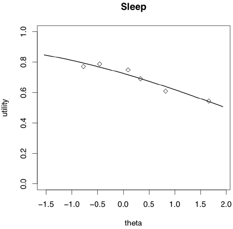
Modeling mean sleep disturbance utilities as a function of the health states. The solid curve is the line of best fit for the model treating health states as a continuous linear variable (i.e., theta in item response theory). The diamonds are the result of treating the health states as factors (i.e., a categorical variable)
Figure 3.
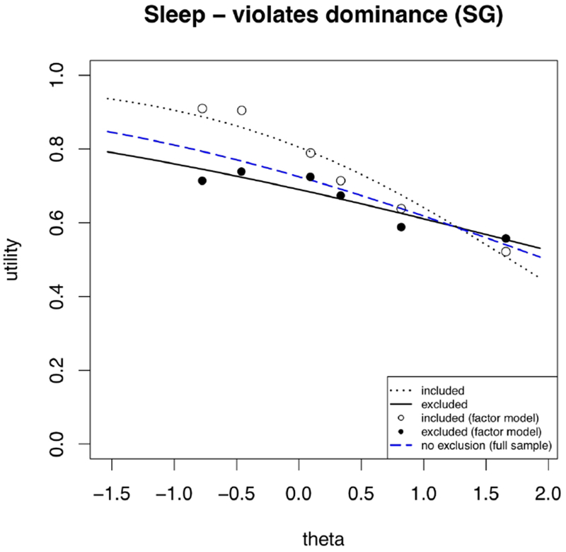
Modeling sleep utilities as a function of health states and the violates-SG criterion, treating health states as continuous (lines) and as factors (dots).
The first column of Table 3 shows regression coefficients for the mean model for all responses to sleep disturbance states (i.e., Equation 1 without the criterion variable). The entries are on the logit (log-odds) scale, so an entry of value x equals on the utility scale. We explain each value in turn.
The value of the constant in the regression table is the log-odds utility (0.969) of the health state described by theta = 0 (the population average), which is sleep of moderate quality. That equals utility of 0.725 (on the 0–1 utility scale). The theta coefficient shows how log-odds utility decreases as sleep disturbance worsens (and theta increases). For example, moving from theta = 0 to theta = 1 reduces utility from 0.725 to 0.618 [= logit−1(0.969 — 0.487) = logit−1(0.482).] As the units are in log-odds, the change in utility caused by a one-unit change in theta depends on where it occurs on the theta scale. Figure 1 shows the conditional mean curve estimated from the model. It also shows the associated factor model (the diamonds), treating the health states as categorical rather than continuous variables.
The numeracy exclusion criterion discards all responses of any participant who scores below 2.5, after averaging the three questions (scored 1–6) on the short form of the Subjective Numeracy Scale (second column of Table 3) (33,34). Figure 1 shows the effects of applying this criterion in two ways. The first applies beta regression separately to the included and excluded responses, seen in the dotted and solid black lines, respectively. The second is the factor model, which presents conditional means of included and excluded responses for each theta value separately, seen in the open and solid black dots, respectively.
The regression models find that participants excluded by numeracy have higher utility for sleep, for all values of theta, compared to participants who have a high score on the numeracy test. That is, those who are excluded reported utility values for intermediate sleep states closer to the utility of the best sleep state. The same result holds for the factor model, except for one value of theta. Given the greater stability of the regression models, which incorporate all data, we focus on them, but discuss the factor model in sensitivity analyses (see Section C3 and C4 in the Appendix). The dashed blue curve is the regression for the full sample, as in Figure 2. The error in estimating the curves depends on the number of responses in each group and their variability (see Table 2 as well as Section C1 and C2 in the Appendix).
Figure 2.
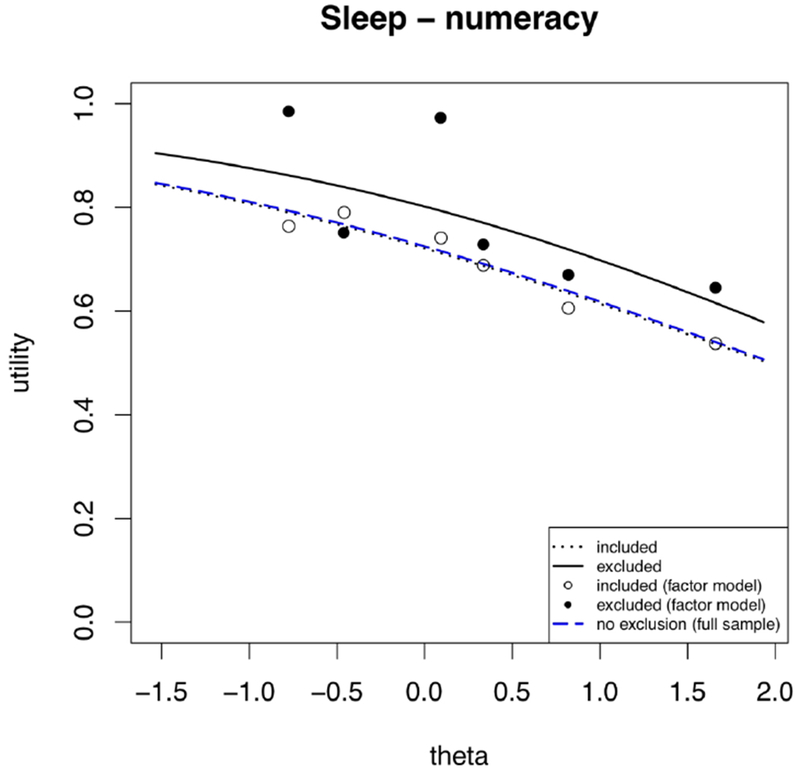
Modeling sleep utilities as a function of health states and the numeracy criterion, treating health states as continuous (lines) and as factors (dots).
Table 2.
Proportion of participants flagged by each criterion, per domain. The proportion of participants in the PROPr data flagged by each criterion from Table 1, per domain. Each column label is one of the seven PROPr domains, with the number of participants assigned to value that domain in parentheses, with the sum 1,164. Each row is one of the core criteria (Table 1), with the percentage of all participants excluded by each criterion in parentheses. Unshaded rows indicate preference-based criteria, shaded rows indicate process-based criteria.
| Exclusion criterion (% excluded in total) | Cognition (n = 166) | Depression (n = 167) | Fatigue (n = 166) | Pain (n = 166) | Physical function (n = 166) | Sleep (n = 166) | Social (n = 167) |
|---|---|---|---|---|---|---|---|
| understanding (14.3%) | 17.5% | 10.8% | 14.5% | 14.5% | 15.1% | 12% | 15% |
| time (15.6%) | 12% | 17.4% | 16.9% | 16.3% | 17.5% | 13.9% | 15% |
| numeracy (7.8%) | 8.4% | 9.0% | 9.0% | 12.7% | 4.2% | 5.4% | 6.0% |
| no-variance (11.8%) | 12.0% | 6.6% | 14.5% | 15.1% | 9.0% | 13.3% | 12.0% |
| low-range (12.2%) | 12.7% | 7.2% | 15.1% | 15.7% | 9.6% | 13.3% | 12.0% |
| lower-tail (44.1%) | 42.2% | 44.9% | 45.8% | 42.8% | 52.4% | 38.0% | 42.5% |
| upper-tail (78.5%) | 78.9% | 77.8% | 80.1% | 74.1% | 77.1% | 83.7% | 77.8% |
| violates-SG (71.6%) | 72.3% | 74.9% | 72.3% | 71.1% | 77.7% | 64.5% | 68.3% |
| dead-all-worst (28.0%) | 28.9% | 25.7% | 26.5% | 30.7% | 24.7% | 28.9% | 30.5% |
| violates-VAS (84.7%) | 85.5% | 80.8% | 88.6% | 80.1% | 89.8% | 85.5% | 82.6% |
The constant corresponds to the utility of a theta score of 0 for participants not excluded by the numeracy criterion (dummy=0). The log-odds value of 0.948 (the constant in Table 3) equals 0.721 on the 0–1 utility scale. The log-odds value of −0.484 for the theta coefficient says that one standard deviation of worse sleep disturbance – for example, from theta=0 to theta=1 -- reduces estimated mean utility from 0.721 [=logit−1(0.948) = 0.721] to 0.614 [=logit−1 (0.948–0.484× 1)= logit−1(0.948 – 0.484) = logit−1(0.464)].
The numeracy coefficient indicates the extent to which the excluded group (solid line in Figure 1) assigned higher values to sleep quality – and the extent to which excluding them reduces the societal utility of sleep quality.
The coefficient for the theta:numeracy interaction term equals the difference in the change in predicted mean utility as theta changes for the groups included and excluded by numeracy. As seen in Figure 2, the sensitivity of the excluded group (solid line) is only slightly more pronounced than that of the non-excluded group (dotted line). The closeness of the models for the full sample (dashed blue) and its non-excluded subgroup (dotted line) reflects the relatively small number excluded by numeracy (Table 2) and the small interaction term.
The violates-SG exclusion criterion discards all responses of participants who assign a higher utility to any health state than to one describing a higher level of functioning. The third column of Table 3 and Figure 3 show the results of applying violates-SG to judgments for the sleep disturbance domain. Unlike numeracy, where the small theta-criterion interaction term and the small number of excluded participants mean relatively parallel utility curves, here, the interaction term and number of excluded participants are both much larger, producing quite different utility functions. Figure 3 shows that excluded participants assigned lower values to high sleep quality, similar values to moderate sleep quality, and higher values to poor sleep quality. Figure 4 shows the full sample curve and reduced sample (included) curves, applying each criterion to the sleep domain responses.
Figure 4.
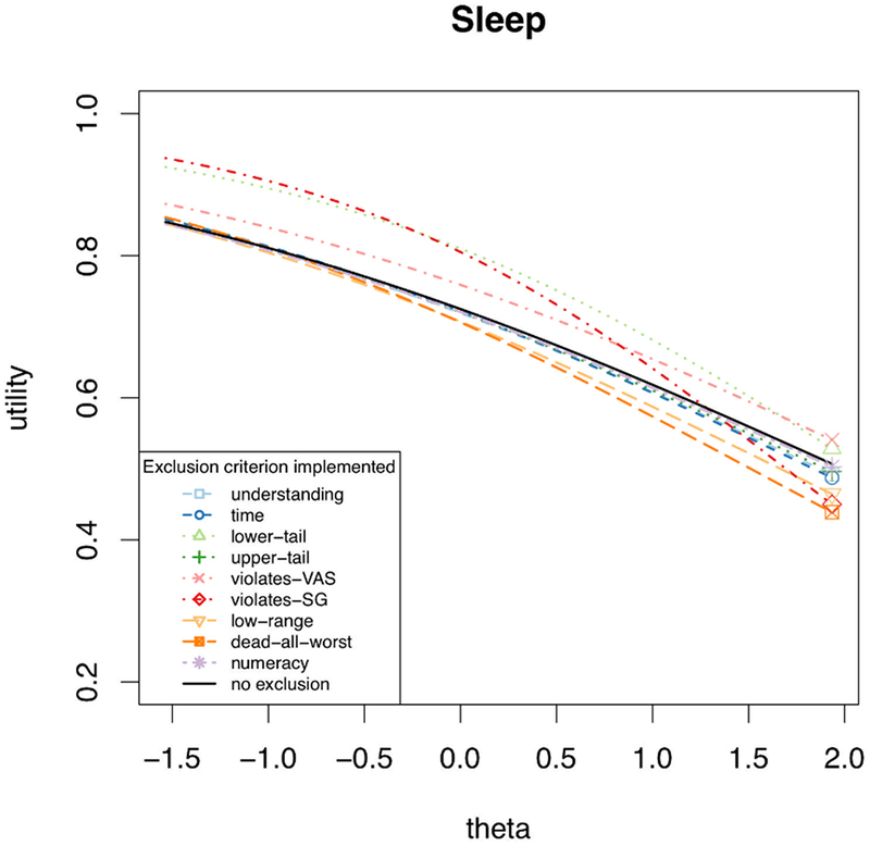
The estimated conditional mean utility curve for sleep, after applying the indicated exclusion criterion (or no exclusion). Note the y-axis begins at 0.2, to magnify the utility curves.
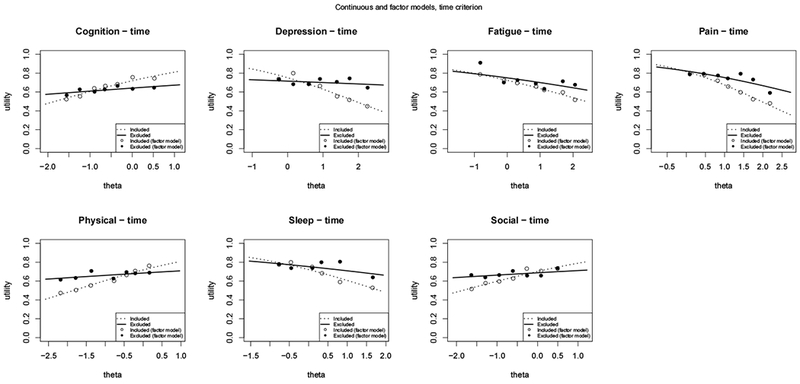
Figure 5 compares the full sample and reduced sample curves for all domains, applying each exclusion criterion (details in the Appendix, Figures C1–C8). Tables C1–C7 in the Appendix summarize the regression coefficients for all domain and criteria combinations.
Figure 5.
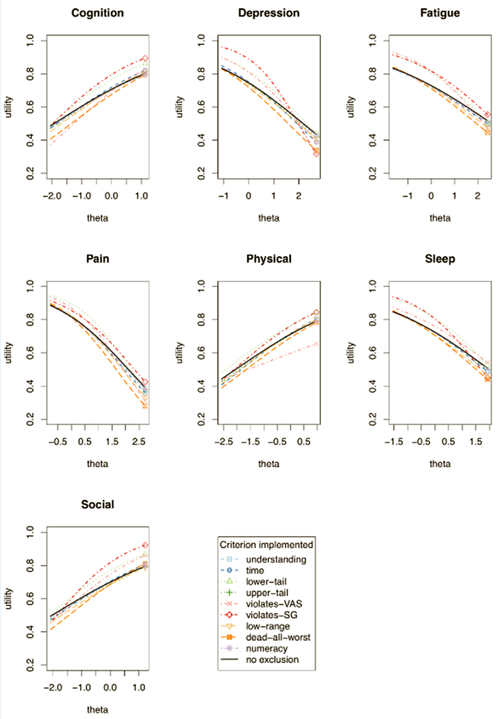
The estimated conditional mean utility for each domain, after applying each exclusion criterion (or no exclusion). Note y-axis starts at 0.2, to magnify the curves.
The patterns revealed in the sensitivity analysis were generally similar to those in the main analysis (see Sections C3–C5 in the Appendix).
Discussion
We begin by discussing the implications of these results for the worked example of sleep disturbance, and then summarize other results, in the form of patterns found across health domains and potential recommendations for selecting exclusion criteria.
Sleep Disturbance Example
As seen in Table 3 and Figure 1, applying the numeracy exclusion criterion lowers the utility curve for sleep disturbance. That could give sleep-related treatments higher priority because each level of sleep is less satisfactory and leaves more room for improvement. If a policy decision is sensitive to the difference, then investigators would need to decide why the excluded responses were different. If less numerate participants were simply less able to perform the standard-gamble task, then excluding them might be justified, by arguing that their preferences are better represented by the responses of society’s more numerate members. However, if the excluded participants genuinely assign higher utility to all health states, then excluding them misrepresents societal utilities and inappropriately increases the value of treatments that improve sleep quality. The analysis of exclusion patterns in the companion paper suggest that the former is the case. The similarity of the slopes of the curves for the full and reduced samples means, however, that exercising the criterion would not affect decisions that depend on treatment effectiveness (or side effects), captured in the change in utility across health states. The small number of excluded participants (5.4%) mitigates the effect of wrongfully excluding (or including) those participants.
Similarly, applying the violates-SG exclusion criterion increases the value of treatments for very poor sleep, because that part of the curve is lower for non-excluded responses. On the other hand, it decreases the value of treatments that make good sleep even better, because that part of the curve is higher. The steeper slope of the utility curve after applying violates-SG makes a unit of improved sleep more valuable, no matter where it occurs. The companion article suggests that participants excluded by violates-SG struggled with the task but were earnestly engaged. Because 64.5% of responses violated this criterion (Table 2), applying it implies a tradeoff between potentially not representing the sample and potentially not representing the preferences of those in it.
Recommendations
Exclusion criteria assume that excluded individuals are better represented by the preferences of the participants who remain than by the ones that they themselves reported. In this and the companion paper, we have analyzed commonly used criteria, in terms of whom they exclude and how they affect utility estimates. Here, we summarize our recommendations for using each exclusion criterion, by examining all criterion-by-domain pairs in Figures C1–C8 of the Appendix.
The need to consider exclusion criteria at all means that more inclusive elicitation procedures are needed. Our recommendations appear in Table 4.
Table 4.
Summary of recommendations for exclusion criteria. We summarize our recommendations for each criterion below, based on our results from this paper and its companion (3). Note that any criterion includes the risk of wrongful exclusion. The magnitude of that risk is partly a function of the number of participants affected by the criterion. The extent to which that varies across studies is an empirical question.
| Exclusion criteria (short-hand) | Recommendations |
|---|---|
| Violates dominance on the SG (violates-SG) | We do not endorse this criterion. Our results suggest it captures many who are engaged with the task. |
| Valued the all-worst state or dead as the same or better than full health (dead-all-worst) | We endorse this criterion. It represents the most egregious violation of dominance, and our analysis suggests a response process for it that is different from violates-SG and more likely to produce responses that are not preferences. |
| Used less than 10% of the utility scale (low-range) | We recommend this criterion as well as more stringent versions of it (e.g., no-variance). Our results support the claim that it captures inattentive responses. |
| In the top 5% of responses for an SG (upper-tail) | We do not endorse the criterion – usually combined with lower-tail – because of the mismatch between the basis for it and our empirical results. |
| In the bottom 5% of responses for an SG (lower-tail) | We do not endorse the criterion – usually combined with upper-tail – because of the mismatch between the basis for it and our empirical results. |
| Score on the Subjective Numeracy Scale of less than 2.5 (numeracy) | We endorse this criterion. However, a researcher must consider any problems with representing the preferences of the less-numerate in their sample with their more numerate counterparts. |
| Self-assessed understanding equal to 1 or 2, on a scale of 1 = “Not at all” to 5 = “Very much” (understanding) | We do not endorse this criterion, as it appears likely that it captures conscientious participants. |
| 15-minute time threshold (time) | We endorse this criterion, as its rationale (inattention) is supported by its empirical effects. |
We begin with the three process-related criteria.
Process-related exclusion criteria
Numeracy.
Applying the numeracy criterion produces a lower utility curve for all domains except depression. As mentioned, the companion article concluded that less numerate participants’ difficulty with the task produces artifactually high estimates. We recommend excluding responses of less numerate participants. Given their small number in the demographically diverse PROPr sample (7.8%), however, the choice might make little practical difference, as in the sleep example (Figure 1).
Time.
This criterion excludes participants who spent less than 15 minutes taking the survey, deemed the minimum for thoughtful responses, based on pre-tests. Across the 7 health domains, the utility curves for those excluded by this criterion were not consistently higher or lower than those for the remaining participants. However, they were consistently flatter. Although that response pattern could reflect insensitivity to health states, the analyses in the companion article suggest that these participants were inattentive. We recommend excluding them. Including them would produce inappropriately flat utility curves, diminishing the value of treatments that improve health states – and underestimating the importance of side effects that degrade health states. They represent 15.6% of the PROPr sample.
Understanding.
This criterion excludes participants who reported not understanding the task. Applying it would have little effect on the elevation of the utility curves, other than lowering that for fatigue, while slightly increasing the slope for all domains. The similarity in the curves suggests that those who reported not understanding the task may have set a higher standard for themselves, rather than actually experiencing more difficulty. As a result, we recommend including them, even if they are uncertain that they should be. They represent 14.3% of the PROPr sample.
Preference-related criteria
Dead-all worst.
This criterion excludes participants whose utility for the dead or all-worst state was not lower than the utility for the best health state. These participants had systematically higher and flatter curves than the others. The companion article (in Box 1) suggests how the mechanics of the standard-gamble interface might have inadvertently led to unduly high responses. We recommend excluding these participants. They represent 28.0% of the PROPr sample.
Violates-SG.
This criterion excludes participants who rated at least one health state more highly than another strictly better health state. For all 7 domains, the utilities of these participants were lower than those of other participants, for most theta values. Their responses showed less curvature on all domains except fatigue and pain. However, the mean utility curves of these participants do not violate dominance, in the sense of decreasing, rather than increasing, as health states improve. The lack of an overall effect suggests that the individual violations reflect the noisiness of a challenging task, consistent with a previous finding that violations are more likely with more similar health states (2,35). That interpretation provides one explanation for our violates-SG and dead-all-worst results in both papers: the former could be capturing many engaged participants trying to distinguish between similar health states, whereas the latter violation involves such distant health states that it is unlikely an engaged participant would produce it. Given the large number of participants with at least one such violation (71.6% of the PROPr sample), we recommend not applying this exclusion criterion.
Upper-tail and lower-tail.
These criteria exclude the highest and lowest 5% of responses, for each health state. As they are the only criteria we considered that exclude individual responses and not entire individuals, we examined differences between those eligible for exclusion by these criteria and those who are not. Most studies that apply these criteria combine them, in a procedure known as 10% trimming. However, the companion article found that they identify different response processes. By definition, upper-tail excludes participants with the highest utility values at a given state, whereas lower-tail excludes participants with the lowest – but they say nothing about their utilities for the states at which they are not among the extremes. For cognition, depression, pain, physical function, sleep disturbance, those excluded by upper-tail have less sensitive utility curves (and equally sensitive for the other three domains). For cognition, depression, fatigue, pain, sleep, and social roles, lower-tail excludes participants whose curves are less sensitive to changes in health states (and equally sensitive for physical function). One difference not captured by the regressions is that a much higher percentage of responses fall in the upper tail than the lower tail, 78.5% vs. 44.1%. Both percentages are much higher than 5% because of ties. Because they disqualify so many responses, standard practice is to sample at random enough eligible responses to make up 5% of the total sample. The large number captured by each supports the need for improved elicitation methods – see also Box 1 in (3). We recommend not applying them, because of the mismatch between their combined rationale and our empirical results (i.e., that they do not act in a completely symmetric manner).
Low-range.
This criterion excludes participants who used less than 10% of the utility scale. Their utility curve is necessarily less sensitive to health states. As a result, removing them increases the sensitivity of the utility curve. Highly similar responses could mean either insensitivity to the health states or inattention. As noted in the companion article, most of these responses were 1, suggesting that participants rushed through the survey, hence were inattentive. As a result, we recommend using this exclusion criterion. It applies to 12.2% of the PROPr sample.
Conclusion
Exclusion criteria for health state preference surveys seek to identify responses that are not valid representations of participants’ preferences. In this article and the companion one, we offer an approach to assessing the properties of exclusion criteria and their impacts on utility estimates. We demonstrate the approach with responses from a nationally representative U.S. sample, evaluating health states on 7 domains from the PROMIS inventory, producing the PROPr scoring system.
The approach has two components. The first, in the companion paper, uses multidimensional scaling (MDS) to characterize the agreement among criteria regarding whom to include and exclude. Applied to the PROPr data, it found differences between the usual rationales of criteria and their empirical effects, such as when two criteria that are typically combined have quite different exclusion patterns (“trimming” the highest and lowest 5% of responses).
The second component of our approach, described here, estimates the impact of applying exclusion criteria on health state utilities. It uses beta regression, a procedure suited to modeling double-bounded variables, such as health utility. Applied to the PROPr data, the beta regression analyses found that some criteria had little impact, because relatively few responses were involved or preferences were similar for the included and excluded groups. It also found criteria that affected the elevation of health utility functions (hence, the acceptability of health states) or their sensitivity to changes in health state (hence, the importance of changes).
Applying these two methods clarifies who is excluded by an exclusion criterion and how it affects the resulting societal health utility estimates. That clarification should help researchers make informed trade-offs between data quality and sample representativeness. It should also help them to inform policy analysts and policy makers how data analytic choices affect health utility estimates and decisions using them.
In addition to contributing new methodologies, the MDS and beta regression results extend previous ones by their inclusiveness. In their systematic review, Engel et al. (2) found only one study that analyzed the effects on utility models of exclusion criteria other than violations of dominance (18).
Nevertheless, our specific results are limited to the exclusion measures studied, the sample (nationally representative U.S.), the 7 health state domains, their measure (PROMIS), the elicitation procedure (standard gamble, preceded by visual analog scale), administration method (online), and implementation (see sample screenshots, Figures A2 and A3, in the Appendix). The effects of changing any of these features is an empirical question.
The standard gamble is attractive because it is rigorously grounded in utility theory (36). Given some participants’ apparent difficulty with the standard gamble, we encourage additional research designed to improve the method, especially for online implementation, with its potential for efficient elicitation from large, representative samples. The need for exclusion criteria is primarily attributable to two related sources: inattentive participants and difficult survey items. We can reduce exclusions by improving the accessibility of our stimuli, which could include more warm-up exercises that train participants to use the stimuli to communicate their preferences. Our methodology offers a systematic way to evaluate alternative designs, whether those be new implementations of widely-used methods or wholly new preference elicitation mechanisms. The better people can understand their tasks, and translate their preferences into those terms, the less need there will be to worry about exclusion criteria.
Acknowledgments
This research was completed at the Division of General Internal Medicine, the University of Pittsburgh, and the Department of Engineering & Public Policy, Carnegie Mellon University. Barry Dewitt received partial support from a Social Sciences and Humanities Research Council of Canada Doctoral Fellowship. Janel Hanmer was supported by the National Institutes of Health through Grant Number KL2 TR001856. Data collection was supported by the National Institutes of Health through Grant Number UL1TR000005. Baruch Fischhoff and Barry Dewitt were partially supported by the Swedish Foundation for the Humanities and Social Sciences. The funding agreements ensured the authors’ independence in designing the study, interpreting the data, writing, and publishing the report.
Appendix A
The PROPr survey
The survey used to collect the data for the PROPr scoring system had the following components:
Consent to participate.
Demographic information.
Participant’s overall self-rated health: excellent, very good, good, fair, or poor [1].
The PROMIS-29 questionnaire [7], plus 4 questions from the Cognition short form [8].
The participant’s self-assessed additional life expectancy.
Valuation of 1 of the 7 health domains, assigned at random.
Task engagement questions.
These are described in more detail in the PROPr technical report [11], available at http://janelhanmer.pitt.edu/PROPr.html.
Figure A.1 shows the qualitative descriptors used to present health states to participants. Figure A.2 shows an example screen from the VAS elicitations. Figure A.3 shows an example screen from a standard gamble elicitation.
Table A.1 provides the theta scores corresponding to the health states valued by participants in the PROPr survey. A theta value is the number associated with the health states on that health state’s underlying domain scale (e.g., pain scale). Table A.2 provides demographic characteristics of the participants in the PROPr survey.
Figure A.1:
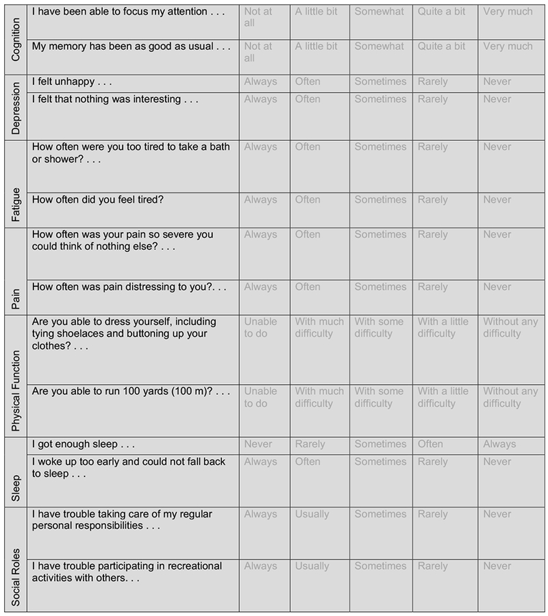
Qualitative descriptions of health states presented to survey participants. A single health state is represented by responses selected at every row. For single-domain health states, the other domains were kept at their highest levels.
Figure A.2:
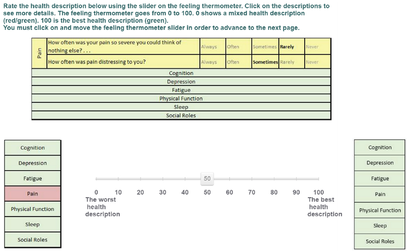
An example valuation, using the visual analogue scale (VAS).
Figure A.3:
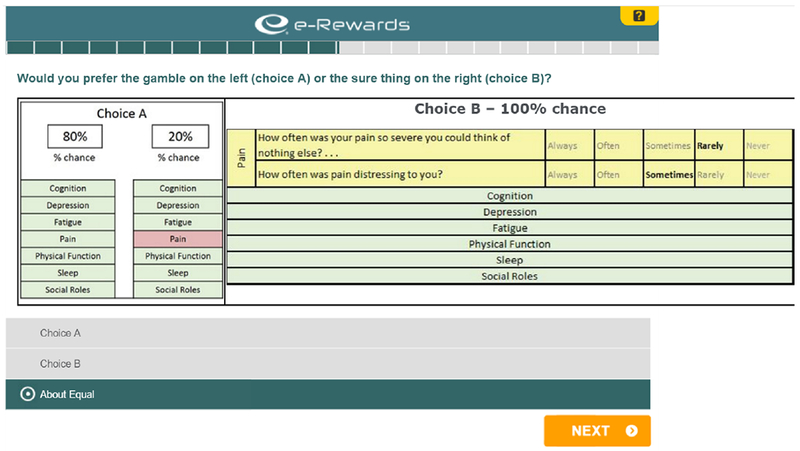
An example valuation, using the standard gamble (SG).
Table A.1: PROMIS theta scores used in PROPr elicitation tasks.
The table shows the theta values corresponding to the health state descriptions valued in the PROPr survey. The levels between the unhealthiest and the healthiest correspond to the intermediate states valued in the elicitation task. The unhealthiest levels, together, define the all-worst state, while the best levels, together, define full health. The disutility corner state for a domain corresponds to the state described by the worst level on that domain, and the best on all others.
| PROMIS Domain | Healthy | … | … | … | … | Unhealthy | |||
|---|---|---|---|---|---|---|---|---|---|
| Cognition | 1.124 | 0.520 | −0.002 | −0.367 | −0.649 | −0.902 | −1.239 | −1.565 | −2.052 |
| Depression | −1.082 | −0.264 | 0.151 | 0.596 | 0.913 | 1.388 | 1.742 | 2.245 | 2.703 |
| Fatigue | −1.648 | −0.818 | −0.094 | 0.303 | 0.870 | 1.124 | 1.688 | 2.053 | 2.423 |
| Pain | −0.773 | 0.100 | 0.462 | 0.827 | 1.072 | 1.407 | 1.724 | 2.169 | 2.725 |
| Physical function | 0.966 | 0.160 | −0.211 | −0.443 | −0.787 | −1.377 | −1.784 | −2.174 | −2.575 |
| Sleep | −1.535 | −0.775 | −0.459 | 0.093 | 0.335 | 0.820 | 1.659 | 1.934 | |
| Social roles | 1.221 | 0.494 | 0.083 | −0.276 | −0.618 | −0.955 | −1.293 | −1.634 | −2.088 |
Table A.2: Participant demographics.
The first column shows the expected demographic characteristics based on the U.S. 2010 Census. The second column shows the demographic characteristics of the participants who completed the survey.
| Gender | U.S. 2010 Census | Total sample (n = 1164) |
|---|---|---|
| Female | 51.0% | 52.7% |
| Male | 49.0% | 47.0% |
| Other | N/A | 0.3% |
| Age | Census | Total |
| 18-24 | 13.0% | 12.0% |
| 25-34 | 17.0% | 18.0% |
| 35-44 | 17.0% | 15.0% |
| 45-54 | 19.0% | 17.0% |
| 55-64 | 16.0% | 17.0% |
| 65-74 | 9.0% | 11.0% |
| 75-84 | 6.0% | 6.0% |
| 85+ | 3.0% | 5.0% |
| Hispanic | Census | Total |
| Yes | 16.0% | 17.0% |
| No | 84.0% | 83.0% |
| Race | Census | Total |
| White | 72.0% | 75.4% |
| AA | 12.0% | 12.5% |
| American Indian | 1.0% | 1.0% |
| Asian | 5.0% | 5.5% |
| Native Hawaiian | 1.0% | 0.2% |
| Other | 6.0% | 3.2% |
| Multiple Races | 3.0% | 2.2% |
| Education for those age 25 and older | Census | Total (n = 1029) |
| Less than high school | 13.9% | 11.9% |
| High school or equivalent | 28.0% | 26.3% |
| Some college, no degree | 21.0% | 21.7% |
| Associate’s degree | 7.9% | 6.9% |
| Bachelor’s degree | 18.0% | 19.4% |
| Graduate or professional degree | 11.0% | 13.8% |
| Income | Census | Total |
| Less than $10,000 | 2.0% | 3.7% |
| $10,000 to less than $15,000 | 4.0% | 3.5% |
| $15,000 to less than $25,000 | 14.0% | 10.3% |
| $25,000 to less than $35,000 | 17.0% | 15.8% |
| $35,000 to less than $50,000 | 20.0% | 18.5% |
| $50,000 to less than $65,000 | 15.0% | 16.4% |
| $65,000 to less than $75,000 | 6.0% | 6.0% |
| $75,000 to less than $100,000 | 10.0% | 11.1% |
| $100,000 or more | 12.0% | 14.7% |
| Self-Rated Health | Census | Total |
| Excellent | N/A | 14.9% |
| Very Good | N/A | 38.7% |
| Good | N/A | 33.1% |
| Fair | N/A | 11.5% |
| Poor | N/A | 1.8% |
Appendix B
Exclusion criteria
Table B.1 provides additional examples of how exclusion criteria can be implemented in the PROPr dataset.
Table B.1: Examples of implementing exclusion criteria in PROPr.
Examples of how to implement the exclusion criteria from Table 1 in the main text of Exclusion I, using the PROPr data. Unless otherwise indicated, valuations refer to the valuations of the single-attribute states. Unshaded rows indicate preference-based criteria, shaded rows indicate process-based criteria.
| Exclusion criterion | Requirements for exclusion |
|---|---|
| Violates dominance on the SG | A participant, using the standard gamble (SG), violates dominance at least once. |
| Violates dominance on the SG, more than twice | A participant, using the standard gamble (SG), violates dominance at least twice. |
| Violates dominance on the SG by more than 10% of the scale | A participant, using the standard gamble (SG), is considered to have violated dominance only if they do so by a difference of more than 0.1 on the utility scale. |
| Violates dominance on the SG by more than 10% of the scale, more than twice | A participant, using the standard gamble (SG), is considered to have violated dominance only if they do so by a difference of more than 0.1 on the utility scale, more than twice. |
| Violates dominance on the VAS | A participant, using the visual analog scale (VAS), violates dominance at least once. |
| Violates dominance on the VAS, more than twice | A participant, using the visual analog scale (VAS), violates dominance at least twice. |
| Violates dominance on the VAS by more than 10% of the scale | A participant, using the visual analog scale (VAS), is considered to have violated dominance only if they do so by a difference of more than 10 on the 0–100 VAS scale. |
| Violates dominance on the VAS by more than 10% of the scale, more than twice | A participant, using the standard gamble (SG), is considered to have violated dominance only if they do so by a difference of more than 10 on the 0–100 VAS scale. |
| Valued the all-worst state or dead as the same or better than full health. | A participant is excluded if they rated the all-worst state or dead as the same or better than full health, using the standard gamble (SG). |
| Used less than 10% of the utility scale | A participant is excluded if their valuations, using the standard gamble (SG), represent less than 10% of the range of the utility scale. |
| Provided the same response to every SG | A participant is excluded if they valued every state the same, using the standard gamble (SG). |
| In the top 5% of responses for an SG | A response is excluded if it falls in the top 5% of responses for that health state, using the standard gamble (SG). |
| In the bottom 5% of responses for an SG | A response is excluded if it falls in the bottom 5% of responses for that health state, using the standard gamble (SG). |
| Score on the Subjective Numeracy Scale of less than 2.5 | A participant is excluded if they scored less than 2.5 on the short form of the Subjective Numeracy Scale (McNaughton, Cavanaugh, Kripalani, Rothman, & Wallston, 2015). |
| Self-assessed understanding equal to 1, on a scale of 1 = “Not at all” to 5 = “Very much” | A participant is excluded if they rated themselves a “1” on the self-assessed understanding question, which occurred after the preference elicitations. |
| Self-assessed understanding equal to 1 or 2, on a scale of 1 = “Not at all” to 5 = “Very much” | A participant is excluded if they rated themselves a “1” or a “2” on the self-assessed understanding question, which occurred after the preference elicitations. |
| 15-minute time threshold | A participant is excluded if they completed the PROPr survey in under 15 minutes. |
Appendix C
Beta regression
Section C.1 shows utility curves – corresponding to Equation 1 in the main text – for all domain and criteria combinations, and their associated regression tables. Section C.2 describes more information on assessing model fit with beta regression. Section C.3 describes the sensitivity analyses for the study presented in the main text in more detail than presented there, and Sections C.4 and C.5 describe the results of those analyses.
C.1. Figures and tables for beta regression models
Figures C.1–C.8 show the estimated mean utility curves for those excluded and not excluded by the 8 criteria studied in the main text, organized by exclusion criterion. Tables C.1–C.7 show the associated regression coefficients of these curves, organized by domain. (For example, Table C.6 completes Table 3 from the main text by adding the rest of the exclusion criteria applied to sleep disturbance.)
C.2. Beta regression model fit
The goodness-of-fit statistic for beta regression models, the pseudo-R2 (also called the proportional reduction of error), reported in Table 3 of the main text, compares the log-likelihoods of the null model (estimating the global mean) and the model under consideration [13]. The value for the model with the numeracy criterion is 0.11. To provide context for that fit, we conducted simulations using data created to be conditionally beta distributed, with two key properties of the present data: (a) a continuous regressor discretized to have six values matching the theta values used in the sleep domain and (b) the same slope (coefficient on theta) as estimated from the real data. The pseudo-R2 of that model is 0.09 (compared to 0.08 for the true model). We repeated the simulation, for violates-SG (third column of Table 3). The pseudo-R2 is 0.22, compared to the observed value of 0.11 in Table 3.
Figure C.1: Beta regression models for violates-SG.
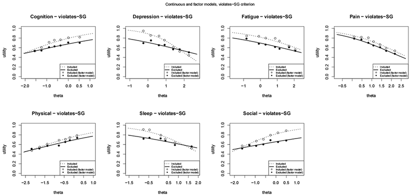
Modeling mean utilities for each domain as a function of theta and the violates-SG criterion.
C.3. Details of the beta regression sensitivity analysis and model-checking
Functional form: Comparing the continuous and factor models provide one assessment of the appropriateness of writing the linear predictor as a linear function of theta in Equation 1 in the main text. The factor model is the extreme of non-linearity, as it calculates the utility value for a given theta using only information from that theta value, and none of its neighbors.
Residual analysis: Residuals for beta regression are constrained by the bounded scale of the beta regression. To examine the fit of the beta model, we simulate a beta distribution data-generating process and fit a correctly specified model. We do this for a case not requiring squeezing, and a case requiring squeezing where beta regression still nearly recovers the correct parameters. We then compare the residual versus fitted values plots with those from our data.
Zero-one inflated beta regression: There is an alternative to the squeezing procedure, that still allows one to take advantage of the benefits of beta regression (e.g., explicit modeling of the variance), called a zero-one inflated beta (ZOIB) model [14]. ZOIB is a mixture model: two binomial models estimated via logistic regression describe the 0 and 1 responses, while a beta regression model describes all the data between 0 and 1.
One disadvantage of the ZOIB approach is that it assumes that there are two processes producing responses, which might not be appropriate depending on the setting: one described by two binomial distributions (producing 1s and 0s) and the other described by a beta distribution. A second is that it is more computationally intensive. A third is that, if we assume each part of the model has the same linear predictor (e.g., η = β0 + β1theta + β2criterion + β3theta : criterion), a ZOIB model is described by twice the number of coefficients than the equivalent squeezed beta regression model, because we are estimating not only the μ and ϕ parameters of the beta but also the means (proportions) of the two logistic regressions.
An advantage of the ZOIB model is that it can better reproduce the data, because of its additional flexibility. In our context, the parsimony of the squeezed beta regression models is useful, because it allows us to easily compare the effects of the different criteria. However, to explore the fit of the squeezed model, we compare it using some of our data to three approaches to ZOIB, which differ in their estimation procedures: a Bayesian approach using Markov chain Monte Carlo (MCMC) sampling, from the R package zoib [14]; separate logistic regressions on the 0/1 data using R’s default function for estimating general linear models, which estimates parameters via iteratively reweighted least squares, combined with a beta regression using the betareg package on the un-squeezed (0,1) data;1 and, a method that uses simulated annealing (a type of numerical optimization) to find the maximum of the joint likelihood of the two logistic regressions and the beta regression [15].
Figure C.2:
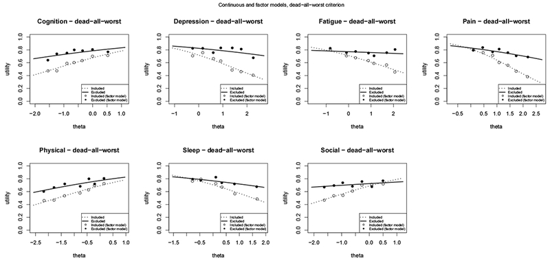
Modeling mean utilities for each domain as a function of theta and the dead-all-worst criterion.
Figure C.3:
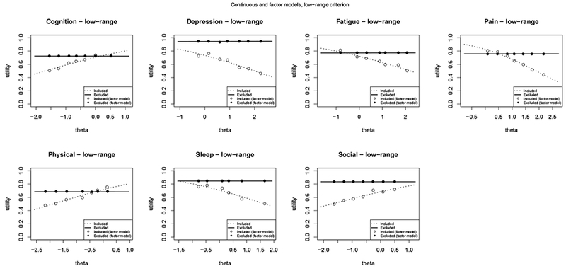
Modeling mean utilities for each domain as a function of theta and the low-range criterion.
Figure C.4:

Modeling mean utilities for each domain as a function of theta and the upper-tail criterion.
Figure C.5:

Modeling mean utilities for each domain as a function of theta and the lower-tail criterion.
Figure C.6:
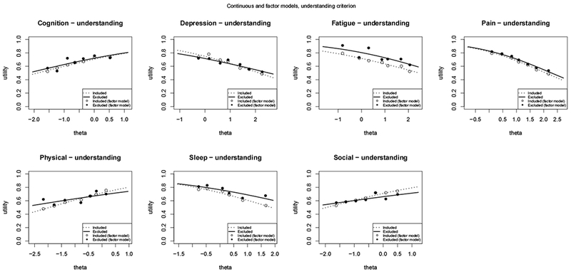
Modeling mean utilities for each domain as a function of theta and the understanding criterion.
Figure C.7:

Modeling mean utilities for each domain as a function of theta and the numeracy criterion.
Figure C.8:
Modeling mean utilities for each domain as a function of theta and the time criterion.
Table C.1:
Coefficients for modeling the mean utility for cognition as a function of theta and the exclusion criterion.
|
Dependent variable: |
|||||||||
|---|---|---|---|---|---|---|---|---|---|
| log-odds utility | |||||||||
| no exclusion | understanding | time | numeracy | low-range | lower-tail | upper-tail | violates-SG | dead-all-worst | |
| intercept | 0.884*** (0.058) | 0.872*** (0.063) | 0.941*** (0.062) | 0.850*** (0.060) | 0.872*** (0.062) | 1.585*** (0.081) | −0.132 (0.107) | 1.359*** (0.119) | 0.737*** (0.067) |
| theta | 0.457*** (0.062) | 0.463*** (0.068) | 0.512*** (0.067) | 0.452*** (0.065) | 0.517*** (0.066) | 0.529*** (0.087) | 0.680*** (0.116) | 0.687*** (0.125) | 0.542*** (0.072) |
| criterion | 0.072 (0.153) | −0.359** (0.172) | 0.580** (0.226) | 0.085 (0.177) | −1.114*** (0.118) | 1.267*** (0.127) | −0.615*** (0.137) | 0.560*** (0.134) | |
| theta:criterion | −0.034 (0.166) | −0.375** (0.190) | 0.237 (0.237) | −0.518*** (0.197) | −0.013 (0.127) | −0.153 (0.137) | −0.287** (0.144) | −0.238 (0.145) | |
| Observations | 1,162 | 1,162 | 1,162 | 1,162 | 1,162 | 1,162 | 1,162 | 1,162 | 1,162 |
| R2 | 0.053 | 0.055 | 0.056 | 0.061 | 0.080 | 0.143 | 0.193 | 0.073 | 0.142 |
| Log Likelihood | 1,609.421 | 1,610.482 | 1,613.717 | 1,613.809 | 1,619.842 | 1,722.767 | 1,732.249 | 1,621.265 | 1,643.453 |
Note:
p<0.1;
p<0.05;
p<0.01
Table C.2:
Coefficients for modeling the mean utility for depression as a function of theta and the exclusion criterion.
|
Dependent variable: |
|||||||||
|---|---|---|---|---|---|---|---|---|---|
| log-odds utility | |||||||||
| no exclusion | understanding | time | numeracy | low-range | lower-tail | upper-tail | violates-SG | dead-all-worst | |
| intercept | 1.072*** (0.066) | 1.095*** (0.069) | 1.106*** (0.072) | 1.091*** (0.069) | 1.018*** (0.067) | 1.852*** (0.094) | 0.589*** (0.114) | 2.074*** (0.144) | 0.938*** (0.074) |
| theta | −0.492*** (0.050) | −0.510*** (0.052) | −0.576*** (0.054) | −0.511*** (0.052) | −0.512*** (0.051) | −0.579*** (0.070) | −0.798*** (0.090) | −1.049*** (0.102) | −0.596*** (0.056) |
| criterion | −0.171 (0.212) | −0.184 (0.175) | −0.181 (0.229) | 1.801*** (0.309) | −1.153*** (0.133) | 0.589*** (0.138) | −1.190*** (0.162) | 0.610*** (0.164) | |
| theta:criterion | 0.146 (0.161) | 0.504*** (0.136) | 0.188 (0.175) | 0.533** (0.242) | 0.016 (0.101) | 0.319*** (0.107) | 0.671*** (0.116) | 0.353*** (0.125) | |
| Observations | 1,169 | 1,169 | 1,169 | 1,169 | 1,169 | 1,169 | 1,169 | 1,169 | 1,169 |
| R2 | 0.089 | 0.088 | 0.118 | 0.090 | 0.130 | 0.179 | 0.163 | 0.103 | 0.231 |
| Log Likelihood | 1,531.725 | 1,534.338 | 1,544.696 | 1,534.016 | 1,578.035 | 1,647.081 | 1,635.614 | 1,555.816 | 1,587.784 |
Note:
p<0.1;
p<0.05;
p<0.01
Table C.3:
Coefficients for modeling the mean utility for fatigue as a function of theta and the exclusion criterion.
|
Dependent variable: |
|||||||||
|---|---|---|---|---|---|---|---|---|---|
| log-odds utility | |||||||||
| no exclusion | understanding | time | numeracy | low-range | lower-tail | upper-tail | violates-SG | dead-all-worst | |
| intercept | 0.989*** (0.055) | 0.930*** (0.059) | 0.964*** (0.060) | 0.958*** (0.058) | 0.949*** (0.060) | 1.856*** (0.082) | 0.023 (0.101) | 1.492*** (0.118) | 0.897*** (0.063) |
| theta | −0.379*** (0.045) | −0.378*** (0.048) | −0.402*** (0.049) | −0.381*** (0.047) | −0.433*** (0.048) | −0.449*** (0.066) | −0.445*** (0.085) | −0.525*** (0.092) | −0.461*** (0.051) |
| criterion | 0.480*** (0.170) | 0.135 (0.152) | 0.389* (0.208) | 0.266 (0.162) | −1.293*** (0.113) | 1.186*** (0.120) | −0.666*** (0.134) | 0.321** (0.130) | |
| theta:criterion | −0.053 (0.135) | 0.151 (0.124) | −0.026 (0.166) | 0.435*** (0.136) | 0.039 (0.092) | 0.015 (0.100) | 0.181* (0.106) | 0.389*** (0.108) | |
| Observations | 1,162 | 1,162 | 1,162 | 1,162 | 1,162 | 1,162 | 1,162 | 1,162 | 1,162 |
| R2 | 0.058 | 0.074 | 0.070 | 0.068 | 0.110 | 0.160 | 0.184 | 0.101 | 0.140 |
| Log Likelihood | 1,661.500 | 1,668.080 | 1,666.015 | 1,665.418 | 1,680.447 | 1,789.760 | 1,764.887 | 1,680.357 | 1,690.973 |
Note:
p<0.1;
p<0.05;
p<0.01
Table C.4:
Coefficients for modeling the mean utility for pain as a function of theta and the exclusion criterion.
|
Dependent variable: |
|||||||||
|---|---|---|---|---|---|---|---|---|---|
| log-odds utility | |||||||||
| no exclusion | understanding | time | numeracy | low-range | lower-tail | upper-tail | violates-SG | dead-all-worst | |
| intercept | 1.498*** (0.083) | 1.486*** (0.090) | 1.493*** (0.090) | 1.460*** (0.089) | 1.557*** (0.090) | 2.167*** (0.114) | 0.817*** (0.133) | 1.774*** (0.164) | 1.461*** (0.096) |
| theta | −0.710*** (0.061) | −0.716*** (0.066) | −0.762*** (0.067) | −0.711*** (0.065) | −0.827*** (0.066) | −0.741*** (0.084) | −0.936*** (0.103) | −0.762*** (0.119) | −0.882*** (0.071) |
| criterion | 0.086 (0.243) | 0.043 (0.234) | 0.371 (0.263) | −0.423* (0.239) | −0.996*** (0.167) | 0.979*** (0.168) | −0.379** (0.191) | 0.120 (0.190) | |
| theta:criterion | 0.028 (0.179) | 0.342** (0.174) | −0.037 (0.191) | 0.828*** (0.183) | −0.068 (0.125) | 0.158 (0.127) | 0.062 (0.139) | 0.525*** (0.142) | |
| Observations | 1,162 | 1,162 | 1,162 | 1,162 | 1,162 | 1,162 | 1,162 | 1,162 | 1,162 |
| R2 | 0.107 | 0.109 | 0.128 | 0.113 | 0.163 | 0.183 | 0.236 | 0.124 | 0.226 |
| Log Likelihood | 1,476.222 | 1,478.527 | 1,485.201 | 1,479.590 | 1,500.599 | 1,584.574 | 1,602.683 | 1,485.398 | 1,524.913 |
Note:
p<0.1;
p<0.05;
p<0.01
Table C.5:
Coefficients for modeling the mean utility for physical function as a function of theta and the exclusion criterion.
|
Dependent variable: |
|||||||||
|---|---|---|---|---|---|---|---|---|---|
| log-odds utility | |||||||||
| no exclusion | understanding | time | numeracy | low-range | lower-tail | upper-tail | violates-SG | dead-all-worst | |
| intercept | 0.906*** (0.065) | 0.928*** (0.071) | 0.933*** (0.072) | 0.903*** (0.067) | 0.924*** (0.068) | 1.652*** (0.102) | −0.113 (0.120) | 1.165*** (0.146) | 0.809*** (0.074) |
| theta | 0.439*** (0.051) | 0.474*** (0.055) | 0.507*** (0.056) | 0.441*** (0.052) | 0.493*** (0.054) | 0.354*** (0.079) | 0.572*** (0.101) | 0.553*** (0.112) | 0.488*** (0.058) |
| criterion | −0.137 (0.183) | −0.155 (0.172) | 0.062 (0.329) | −0.162 (0.226) | −1.038*** (0.134) | 1.322*** (0.143) | −0.343** (0.163) | 0.413*** (0.159) | |
| theta:criterion | −0.213 (0.145) | −0.395*** (0.137) | −0.029 (0.257) | −0.496*** (0.182) | 0.180* (0.106) | −0.071 (0.118) | −0.149 (0.126) | −0.151 (0.124) | |
| Observations | 1,162 | 1,162 | 1,162 | 1,162 | 1,162 | 1,162 | 1,162 | 1,162 | 1,162 |
| R2 | 0.072 | 0.076 | 0.089 | 0.072 | 0.094 | 0.183 | 0.221 | 0.085 | 0.127 |
| Log Likelihood | 1,646.134 | 1,649.067 | 1,652.680 | 1,646.439 | 1,658.481 | 1,772.655 | 1,757.685 | 1,657.071 | 1,667.841 |
Note:
p<0.1;
p<0.05;
p<0.01
Table C.6:
Coefficients for modeling the mean utility for sleep disturbance as a function of theta and the exclusion criterion.
|
Dependent variable: |
|||||||||
|---|---|---|---|---|---|---|---|---|---|
| log-odds utility | |||||||||
| no exclusion | understanding | time | numeracy | low-range | lower-tail | upper-tail | violates-SG | dead-all-worst | |
| intercept | 0.969*** (0.050) | 0.940*** (0.053) | 0.952*** (0.054) | 0.948*** (0.051) | 0.883*** (0.053) | 1.607*** (0.068) | 0.115 (0.096) | 1.419*** (0.093) | 0.877*** (0.059) |
| theta | −0.487*** (0.056) | −0.502*** (0.059) | −0.518*** (0.060) | −0.484*** (0.057) | −0.530*** (0.059) | −0.394*** (0.076) | −0.571*** (0.114) | −0.837*** (0.096) | −0.580*** (0.065) |
| criterion | 0.237 (0.160) | 0.165 (0.146) | 0.448* (0.241) | 0.820*** (0.168) | −1.118*** (0.103) | 0.972*** (0.111) | −0.618*** (0.111) | 0.318*** (0.114) | |
| theta:criterion | 0.117 (0.178) | 0.291* (0.165) | −0.073 (0.260) | 0.530*** (0.196) | −0.235** (0.116) | 0.061 (0.130) | 0.486*** (0.118) | 0.322** (0.128) | |
| Observations | 996 | 996 | 996 | 996 | 996 | 996 | 996 | 996 | 996 |
| R2 | 0.076 | 0.086 | 0.083 | 0.081 | 0.151 | 0.185 | 0.169 | 0.111 | 0.126 |
| Log Likelihood | 1,561.564 | 1,564.391 | 1,566.070 | 1,563.459 | 1,584.627 | 1,666.886 | 1,634.717 | 1,581.657 | 1,575.390 |
Note:
p<0.1;
p<0.05;
p<0.01
Table C.7:
Coefficients for modeling the mean utility for social roles as a function of theta and the exclusion criterion.
|
Dependent variable: |
|||||||||
|---|---|---|---|---|---|---|---|---|---|
| log-odds utility | |||||||||
| no exclusion | understanding | time | numeracy | low-range | lower-tail | upper-tail | violates-SG | dead-all-worst | |
| intercept | 0.848*** (0.056) | 0.892*** (0.061) | 0.859*** (0.061) | 0.837*** (0.057) | 0.769*** (0.059) | 1.699*** (0.079) | 0.057 (0.102) | 1.501*** (0.110) | 0.788*** (0.066) |
| theta | 0.415*** (0.059) | 0.454*** (0.064) | 0.463*** (0.063) | 0.425*** (0.060) | 0.452*** (0.062) | 0.424*** (0.083) | 0.679*** (0.111) | 0.802*** (0.110) | 0.544*** (0.069) |
| criterion | −0.225 (0.155) | −0.069 (0.156) | 0.179 (0.245) | 0.843*** (0.197) | −1.294*** (0.114) | 0.974*** (0.121) | −0.852*** (0.128) | 0.180 (0.124) | |
| theta:criterion | −0.206 (0.165) | −0.350** (0.166) | −0.172 (0.258) | −0.452** (0.213) | 0.085 (0.121) | −0.264** (0.131) | −0.481*** (0.130) | −0.417*** (0.131) | |
| Observations | 1,169 | 1,169 | 1,169 | 1,169 | 1,169 | 1,169 | 1,169 | 1,169 | 1,169 |
| R2 | 0.046 | 0.045 | 0.053 | 0.051 | 0.118 | 0.173 | 0.170 | 0.079 | 0.104 |
| Log Likelihood | 1,615.652 | 1,620.772 | 1,618.772 | 1,617.564 | 1,645.881 | 1,779.435 | 1,708.061 | 1,638.875 | 1,639.256 |
Note:
p<0.1;
p<0.05;
p<0.01
C.4. Summary results of the beta regression sensitivity analysis and model-checking
Functional form: As described earlier, comparing the squeezed and ZOIB models that are linear in theta to their associated factor models – where theta is treated as a categorical variable – allows us to test the linearity assumption. For example, the model of those not excluded by numeracy tracks its associated factor model (open dots) well, while the model of those excluded (the solid curve) has some large differences with its factor model (solid dots). This demonstrates that there could be a model that is non-linear in theta and has a better fit for the excluded. Overall, however, most of the continuous models across the domains and the exclusion criteria track their factor counterparts well.
Residual analysis and c) Zero-one inflated (ZOIB) regression: Examining the residuals of our main models (Figures C.1–C.8) shows that they systematically vary from those expected from a conditionally beta-distributed random variable because of the number of 0s and 1s in the data at every value of theta. Moving to the ZOIB models necessarily produces a better fit. However, differences between the included and excluded groups remain, and are, in fact, more pronounced in the ZOIB models. Thus, we believe the squeezed models provide good within-sample comparisons for the main models (Equation 1 in the main text), which are the focus of our study.
C.5. Detailed discussion of the beta regression sensitivity analyses
C.5.1. Residual analysis
The correctly specified beta model with no squeezing shows how residuals in a beta regression are affected by the boundedness of the beta distribution (Figure C.9). Large residuals are only possible near the endpoints. For example, when the fitted values approach 1, the beta distribution – which always places some probability density over the whole open interval – will sometimes produce small values, producing large negative residuals. In the figure, the residuals “step down” as one moves to the right because the beta is skewed unless the two shape parameters are equal, which necessitates a (fitted) mean of 0.5. Otherwise, a mean value less than 0.5 necessitates a right skew, and one greater than 0.5 necessitates a left skew, producing many positive and negative residuals, respectively.
The residuals versus fitted values plot for the correctly specified beta model requiring squeezing, in which beta regression nearly recovers the correct coefficients, shows nearly the same pattern (Figure C.10). That provides us with confidence that squeezing can work well.
Figure C.11 shows residuals versus fitted values for the model of cognition utilities as a function of theta and the time criterion, i.e., whose mean is modeled by:
It shows a similar pattern to Figure C.9 and Figure C.10. However, the columns of residuals at each fitted value have much more consistent length. That is due to the fact that every observed conditional distribution has some 0s and 1s in the data. The spread of the residuals for a fixed fitted value is discrete and often evenly spaced because of the SG elicitation method: utilities could only be given for every 0.05 of the 0-1 utility scale. Notice, too, that the fitted values start just above 0.5, in contrast to our simulations. That is, in our data we are never modeling distributions whose means are close to 0.
Figure C.9: Residuals versus fitted values for a simulated, correctly specified beta model.
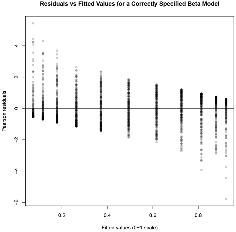
Plot of residuals versus fitted values for a simulated, correctly specified beta model, where beta regression recovers the correct parameters.
Figure C.10: Residuals versus fitted values for a simulated, correctly specified beta model requiring squeezing.
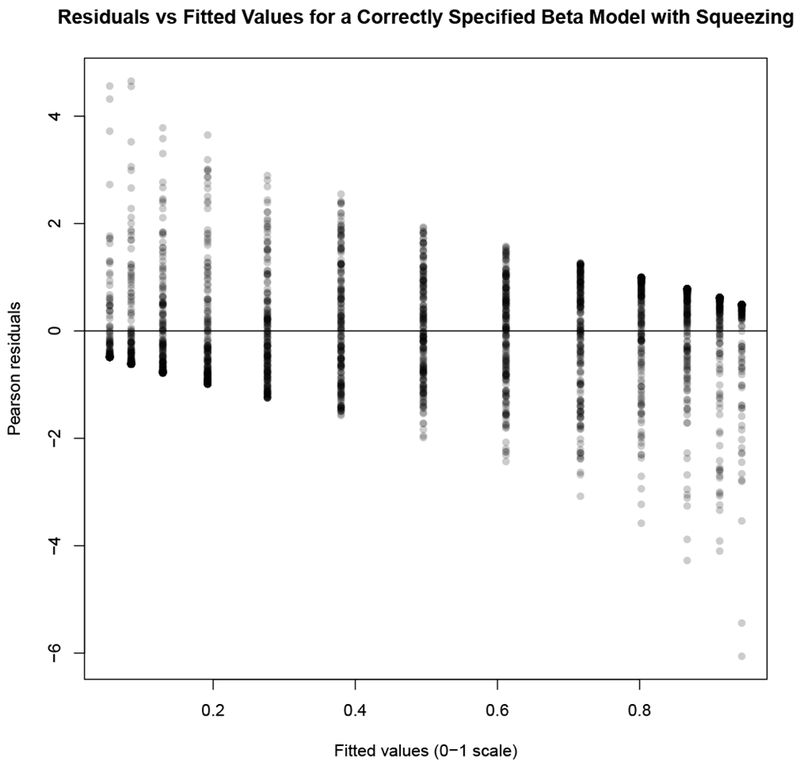
Plot of residuals versus fitted values for a simulated, correctly specified beta model.
Figure C.11: Residuals versus fitted models for cognition as a function of theta and time.
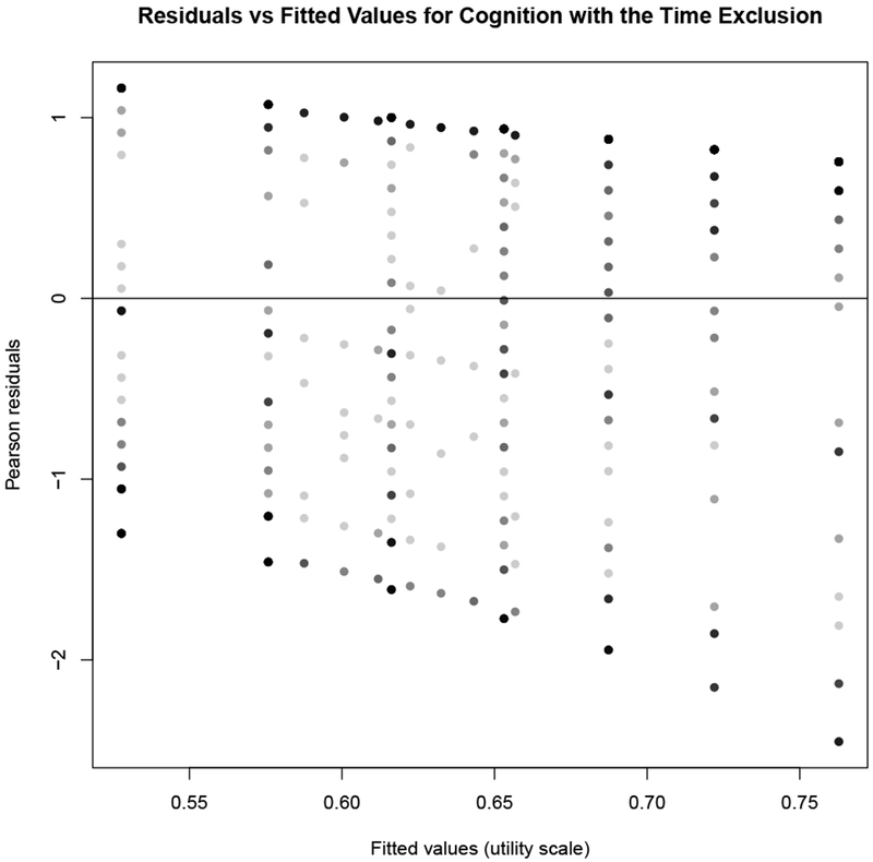
Plot of residuals versus fitted values for the squeezed model .
As a comparison, Figure C.12 shows the residuals versus fitted values for the same model using the cognition data and excluding the 0s and 1s from the dataset – and thus not requiring squeezing. The pattern is very similar to the squeezed model, although there is a more pronounced lowering of the columns of residuals, more closely matching the residual plot of the correctly specified model (Figure C.9). Note, too that the range of fitted values is shifted compared to Figure C.11, and that we do not get close to either endpoint of the scale. There are significantly more 1s than 0s – 574 versus 150 in the cognition domain – and so removing all the 0s and 1s shifts the (fitted) means downwards.
Figure C.12: Residuals and fitted values for cognition utilities as a function of theta and time, no 0s or 1s in the data.
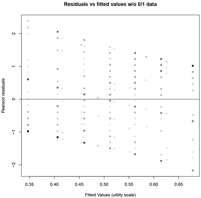
Plot of residuals versus fitted values for the model , using the cognition data without the 0 and 1 responses. (Note this would be the beta portion of the associated ZOIB model.)
Given the patterns of residuals, we believe beta regression provides a useful method for summarizing our data. Although it does not appear that the conditional distributions are exactly beta distributed given our covariates, the general shape of the residual plots reflects some of the key structural features of correctly-specified beta regressions.
We also believe the squeezing procedure is theoretically legitimate for our data. By assumption, the utilities are on an interval scale; more importantly, they are not on a ratio scale. Thus, the 0 is not an absolute, as it would be in a scale for mass or length. In fact, throughout the estimation of the PROPr scoring system [16], we often translate between different utility scales where 0 corresponds to the utility of various states (e.g., dead, the allworst state). Therefore, moving the 0s in the data to 0.5/n via a linear transformation is conceptually equivalent to the other translations of 0s that occur throughout the PROPr scoring system: the interval-scale properties of the data are retained, but the data is transformed for modeling purposes.
By construction, a theta value outside of its domain endpoints – that is, outside of the extreme values in Table A.1 – is given a utility equal to 0 or 1 (depending on which side of the scale it lies). The societal valuation of a state – usually taken to be a mean value – is always between the endpoints, and in practice never equals those extremes, unless it is one of the pre-defined endpoints (i.e., full health and the all-worst state or dead). Thus, making it impossible for an intermediate state to have predicted mean utility of 0 or 1 is not, within the context of health state valuation studies, an unusual assumption.
C.5.2. Zero-one inflated beta (ZOIB) models
To further investigate the squeezing method used in our modeling, we used the data from the cognition domain and compared its results with those of the three ZOIB alternative models. (Recall that, if squeezing were unnecessary, the ZOIB models would reduce to normal beta regression.)
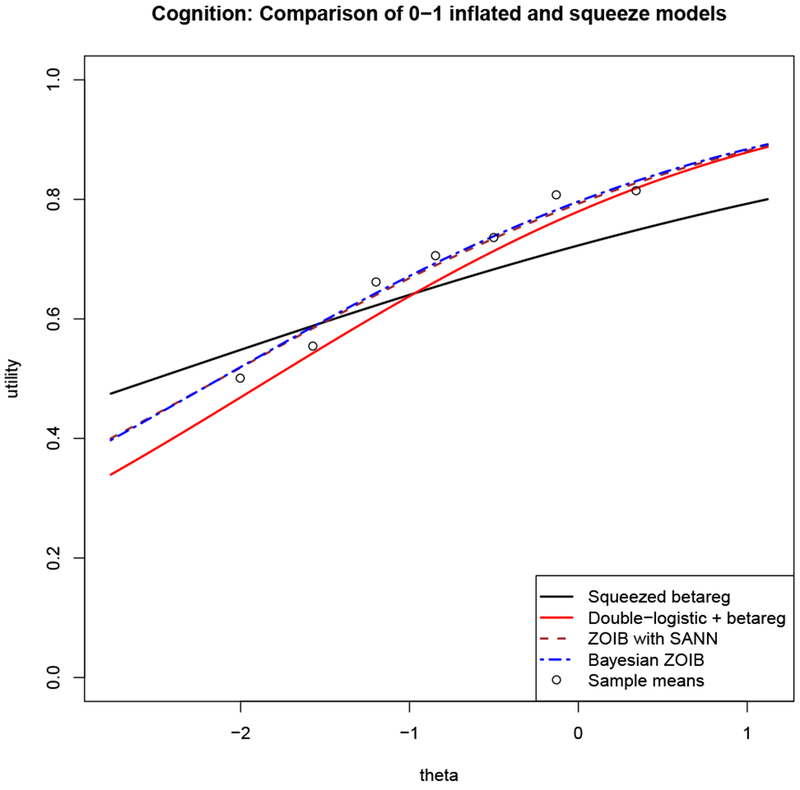
We estimated conditional mean curves for the four models where the linear predictor is only theta (i.e., where there are only two coefficients, the intercept and the slope on theta). Figure C.13 shows the squeezed model (solid black), the double-logistic plus beta version of the ZOIB model (solid red), the Bayesian ZOIB model (dashed brown), the ZOIB model estimated via simulated annealing (dashed blue), and the sample mean utilities of the un-squeezed data (dots). The deviations between the black curve and the sample means suggest some bias in the squeezed model. The Bayesian ZOIB and ZOIB estimated via simulated annealing are almost collinear, and closely reproduce the sample means. The double-logistic plus beta regression have a shape like the two other ZOIB models, but a different intercept.
We also estimated conditional mean curves for the four models where the linear predictor included an exclusion criteria (time), as in the models from the main text. These curves, two for each model – one for those participants excluded by time and one for those left included in the sample – are plotted for each method in Figure C.14. The double-logistic plus beta regression (red) and Bayesian ZOIB (blue) are almost collinear, while the included curve of the ZOIB using simulated annealing (dotted brown) is close to the included curve of the other two ZOIB models, but its excluded curve (solid brown) is further from their excluded curves. The two parts of the squeezed results (black) have a similar shape to the others, but show less extreme slopes in both curves than the ZOIB models, and also show the bias in the excluded (solid) and included (dotted) curves that is seen in Figure C.13.
Figure C.13: Comparison of ZOIB estimation techniques using the cognition data.
A comparison of beta regression on squeezed data (black) and three methods to estimate zero-one inflated beta (ZOIB) models: two logistic regressions on the 0-1 data plus a beta regression on the (0, 1) data (solid red), ZOIB estimated using simulated annealing for maximum likelihood estimation (dashed brown), and a Bayesian ZOIB approach that uses Markov chain Monte Carlo sampling to produce coefficient estimates (dashed blue). The sample means from the data are plotted as points. Every component of every model has the same linear predictor, η = β0 + β1theta.
We implemented the ZOIB models to see the effect of modeling the untransformed data, and compare those models with our main, squeezed models. As seen in Figure C.13, the ZOIB models more closely recover the sample means, which are unbiased estimates of the conditional mean utilities. As there are many 0s and 1s in the data, squeezing them into data in the open interval (0,1) then requires the optimization algorithm to search for beta parameters that will produce many high and low values, and recover the mid-range of values as well. Unless the shape of the empirical distribution of the data (0,1) has peaks at the extremes, this procedure will necessarily do a worse job at recovering the shape of the (0,1) data, as a beta distribution cannot take on every shape imaginable (e.g., it can have at most two modes). The ZOIB models fit a beta regression on only the data in the open interval (0,1), allowing its beta regression to have fewer constraints. Thus, the differences could be caused by squeezing, or the different model assumptions (i.e., the multiple data-generating processes in ZOIB models) or even over-fitting from the more flexible ZOIB models, or by a combination of factors.
In Figure C.14, where the model also includes the interaction, we see that the differences between the included and excluded curves are more pronounced than in the squeezed beta regression. This could be because squeezing brings all the data closer together, thus diminishing the differences between otherwise untransformed utilities. It is promising that the general shapes of the curves are the same in the squeezed and the ZOIB models, and that any relationships are only more pronounced in the more complicated models. Thus, we believe it is more likely we have missed an effect of the exclusion criteria than produced one that would disappear with a ZOIB analysis. Again, two of the ZOIB estimation procedures (the Bayesian and double-logistic plus beta regression) closely recover the sample means.
Based on the results of our comparisons, we believe our squeezed models are best interpreted as parsimonious descriptions of the relationships between utility, health domains (i.e., theta), and exclusion criteria, allowing within-sample comparisons of those relationships, rather than as descriptions of mean population utility estimates. Future work is needed to determine the role of the potential causes of the differences seen between the ZOIB and squeezed models, which include the squeezing, the (in)appropriateness of the beta distribution for describing the data conditional on our chosen covariates, and the extra parameters estimated in the ZOIB models. Moving to the ZOIB models in all aspects of the work could improve the modeling, but would require additional insight to interpret these complicated models for those who wish to use them to inform their survey design - in contrast to those who want to run their own ZOIB models, who might appreciate the thorough methodological discussion. It is unclearwhether there is a large (or any) intersection of these two groups, so care must be taken when proceeding with an even more complex modeling strategy.
Figure C.14: Comparison of ZOIB estimation techniques using the cognition data and time.
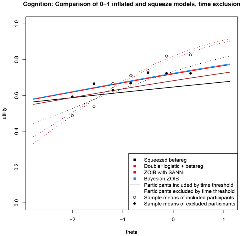
A comparison of beta regression on squeezed data (black) and the same model estimated using three different methods for zero-one inflated beta (ZOIB) regression on the un-squeezed data: two logistic regressions on the 0-1 data plus a beta regression on the (0, 1) data (red), ZOIB estimated using simulated annealing for maximum likelihood estimation (brown), and a Bayesian ZOIB approach that uses Markov chain Monte Carlo sampling to produce coefficient estimates (blue). The solid curves show the estimated conditional mean values for those participants excluded by the time criterion; the dashed curves show the estimated conditional mean values for those participants left in the sample. Every component of every model has the same linear predictor, η = β0 + β1theta + β2criterion + β3theta : criterion.
Footnotes
We will refer to this method, which uses the glm() function in R for the two logistic models and betareg() in the betareg package for estimating the beta model, as the “double-logistic plus beta” version of ZOIB, because it estimates coefficients by running those models separately. Of course, formally, the other methods are also a mixture of two logistic regressions and a beta regression, but their implementation in R differs from simply combining glm() and betareg().
Contributor Information
Barry Dewitt, Department of Engineering & Public Policy, Carnegie Mellon University, Pittsburgh, PA.
Baruch Fischhoff, Department of Engineering & Public Policy and the Institute for Politics and Strategy, Carnegie Mellon University, Pittsburgh, PA.
Alexander L. Davis, Department of Engineering & Public Policy, Carnegie Mellon University, Pittsburgh, PA.
Stephen B. Broomell, Department of Social and Decision Sciences, Carnegie Mellon University, Pittsburgh, PA.
Mark S. Roberts, Department of General Internal Medicine, University of Pittsburgh Medical Center, Pittsburgh, PA; Department of Health Policy and Management, University of Pittsburgh, Pittsburgh, PA.
Janel Hanmer, Department of General Internal Medicine, University of Pittsburgh Medical Center, Pittsburgh, PA.
References
- 1.Wilson IB, Cleary PD. Linking clinical variables with health-related quality of life: A conceptual model of patient outcomes. JAMA. 1995;273(1):59–65. [PubMed] [Google Scholar]
- 2.Engel L, Bansback N, Bryan S, Doyle-Waters MM, Whitehurst DGT. Exclusion Criteria in National Health State Valuation Studies: A Systematic Review. Med Decis Mak [Internet]. 2016;36(7):798–810. Available from: http://www.ncbi.nlm.nih.gov/pubmed/26209475 [DOI] [PubMed] [Google Scholar]
- 3.Dewitt B, Fischhoff B, Davis A, Broomell SB, Roberts MS, Hanmer J. Exclusion criteria as measurements I: Identifying invalid responses. 2019. [DOI] [PMC free article] [PubMed]
- 4.Cella D, Yount S, Rothrock N, Gershon R, Cook K, Reeve B, et al. The Patient-Reported Outcomes Measurement Information System (PROMIS): Progress of an NIH Roadmap Cooperative Group During its First Two Years. Med Care. 2007;45(5):3–11. [DOI] [PMC free article] [PubMed] [Google Scholar]
- 5.Dewitt B, Feeny D, Fischhoff B, Cella D, Hays RD, Hess R, et al. Estimation of a Preference-Based Summary Score for the Patient-Reported Outcomes Measurement Information System: The PROMIS®-Preference (PROPr) Scoring System. Med Decis Mak [Internet]. 2018;0272989X1877663. Available from: http://www.ncbi.nlm.nih.gov/pubmed/29944456%0Ahttp://journals.sagepub.com/doi/10.1177/0272989X18776637 [DOI] [PMC free article] [PubMed]
- 6.Keeney RL, Raiffa H. Decisions with multiple objectives: Preferences and value tradeoffs. New York, NY: John Wiley & Sons; 1976. [Google Scholar]
- 7.Neumann PJ, Saunders Gd, Russell LB, Siegel JE, Ganiats TG, editors. Cost-Effectiveness in Health and Medicine. Second New York: Cambridge University Press; 2016. [Google Scholar]
- 8.Feeny D, Furlong W, Torrance GW, Goldsmith CH, Zhu Z, DePauw S, et al. Multiattribute and single-attribute utility functions for the Health Utilities Index Mark 3 system. Med Care. 2002;40(2):113–28. [DOI] [PubMed] [Google Scholar]
- 9.Rabin R, Charro F De. EQ-SD: a measure of health status from the EuroQol Group. Ann Med 2001. ;33(5):337–43. [DOI] [PubMed] [Google Scholar]
- 10.Nord E Cost-Value Analysis of Health Interventions: Introduction and Update on Methods and Preference Data. Pharmacoeconomics. 2014;33(2):89–95. [DOI] [PubMed] [Google Scholar]
- 11.Hanmer J, Dewitt B. PROMIS-Preference (PROPr) Score Construction -- A Technical Report [Internet]. 2017. Available from: janelhanmer.pitt.edu/PROPr.html
- 12.Hanmer J, Cella D, Feeny D, Fischhoff B, Hays RD, Hess R, et al. Selection of key health domains from PROMIS® for a generic preference-based scoring system. Qual Life Res 2017;1–9. [DOI] [PMC free article] [PubMed] [Google Scholar]
- 13.Hanmer J, Cella D, Feeny D, Fischhoff B, Hays RD, Hess R, et al. Evaluation of options for presenting health-states from PROMIS® item banks for valuation exercises. Qual Life Res [Internet]. 2018;27(7):1835–43. Available from: http://link.springer.com/10.1007/s11136-018-1852-1 [DOI] [PMC free article] [PubMed] [Google Scholar]
- 14.Feeny D A Utility Approach to the Assessment of Health-Related Quality of Life. Med Care. 2000;38(9). [DOI] [PubMed] [Google Scholar]
- 15.Lamers LM, Stalmeier PFM, Krabbe PFM, Busschbach JJV. Inconsistences in TTO and VAS Values for EQ-5D Health States. Med Decis Mak 2006;26(2):173–81. [DOI] [PubMed] [Google Scholar]
- 16.Johnson JA, Ergo A, Coons SJ, Szava-Kovats G. Valuation of the EuroQOL (EQ-5D) Health States in an Adult US Sample. Pharmacoeconomics. 1998;13(4):421–33. [DOI] [PubMed] [Google Scholar]
- 17.Torrance GW, Feeny D, Furlong WJ, Barr RD, Zhang Y, Wang Q. Multiattribute utility function for a comprehensive health status classification system: Health Utilities Index Mark 2. Med Care. 1996;34(7):702–22. [DOI] [PubMed] [Google Scholar]
- 18.Bansback N, Tsuchiya A, Brazier J, Anis A. Canadian valuation of EQ-5D health states: Preliminary value set and considerations for future valuation studies. PLoS One. 2012;7(2). [DOI] [PMC free article] [PubMed] [Google Scholar]
- 19.Devlin nJ, Hansen P, Kind P, Williams A. Logical inconsistencies in survey respondents’ health state valuations - A methodological challenge for estimating social tariffs. Health Econ 2003;12(7):529–44. [DOI] [PubMed] [Google Scholar]
- 20.Pullenayegum EM, Tarride JE, Xie F, Goeree R, Gerstein HC, O’Reilly D. Analysis of health utility data when some subjects attain the upper bound of 1: Are tobit and CLAD models appropriate? Value Heal [Internet]. 2010;13(4):487–94. Available from: 10.1111/j.1524-4733.2010.00695.x [DOI] [PubMed] [Google Scholar]
- 21.Smithson M, Verkuilen J. A better lemon squeezer? Maximum-likelihood regression with beta-distributed dependent variables. Psychol Methods. 2006;11(1):54–71. [DOI] [PubMed] [Google Scholar]
- 22.Paolino P Maximum Likelihood Estimation of Models with Beta-Distributed Dependent Variables. Polit Anal [Internet]. 2001;9(4):325–46. Available from: http://pan.oxfordjournals.org/cgi/doi/10.1093/oxfordjournals.pan.a004873 [Google Scholar]
- 23.Cribari-Neto F, Zeileis A. Beta Regression in R. J Stat Softw 2010;34(2):1–24. [Google Scholar]
- 24.Verkuilen J, Smithson M. Mixed and Mixture Regression Models for Continuous Bounded Responses Using the Beta Distribution. J Educ Behav Stat [Internet]. 2012;37(1):82–113. Available from: http://jeb.sagepub.com/cgi/doi/10.3102/1076998610396895 [Google Scholar]
- 25.Furlong W, Feeny D, Torrance GW, Goldsmith CH, DePauw S, Zhu Z, et al. Multiplicative Multi-Attribute Utility Function for the Health Utilities Index Mark 3 (HUI3) System: A Technical Report. 1998. (McMaster University Centre for Health Economics and Policy Analysis Working Paper; ). Report No.: 98-11. [Google Scholar]
- 26.Dewitt B, Davis A, Fischhoff B, Hanmer J. An Approach to Reconciling Competing Ethical Principles in Aggregating Heterogeneous Health Preferences. Med Decis Mak [Internet]. 2017;0272989X1769699. Available from: http://journals.sagepub.com/doi/10.1177/0272989X17696999 [DOI] [PMC free article] [PubMed]
- 27.Torrance GW, Boyle MH, Horwood SP. Application of multi-attribute utility theory to measure social preferences for health states. Oper Res 1982;30(6):1043–69. [DOI] [PubMed] [Google Scholar]
- 28.Liu H, Cella D, Gershon R, Shen J, Morales LS, Riley W, et al. Representativeness of the Patient-Reported Outcomes Measurement Information System Internet panel. J Clin Epidemiol [Internet]. 2010;63(11):1169–78. Available from: 10.1016/jjclinepi.2009.11.021 [DOI] [PMC free article] [PubMed] [Google Scholar]
- 29.Shalizi CR. Advanced Data Analysis from an Elementary Point of View [Internet]. Cambridge, England: Cambridge University Press; Available from: http://www.stat.cmu.edu/~cshalizi/ADAfaEPoV [Google Scholar]
- 30.Myers RH, Montgomery DC, Vining GG, Robinson TJ. Generalized linear models: with applications in engineering and the sciences. John Wiley & Sons; 2012. [Google Scholar]
- 31.Ellsberg D. Classic and Current Notions of “Measurable Utility.” Econ J. 1954;64(255):528–56. [Google Scholar]
- 32.Koebberling V Strength of preference and cardinal utility. Econ Theory. 2006;27(2):375–91. [Google Scholar]
- 33.Fagerlin A, Zikmund-Fisher BJ, Ubel PA, Jankovic A, Derry HA, Smith DM. Measuring numeracy without a math test: Development of the Subjective Numeracy Scale. Med Decis Mak [Internet]. 2007. [cited 2014 Jun 3];27(5):672–80. Available from: http://www.ncbi.nlm.nih.gov/pubmed/17641137 [DOI] [PubMed] [Google Scholar]
- 34.McNaughton CD, Cavanaugh KL, Kripalani S, Rothman RL, Wallston KA. Validation of a Short, 3-Item Version of the Subjective Numeracy Scale. Med Decis Mak [Internet]. 2015;35(8):932–6. Available from: http://mdm.sagepub.com/cgi/doi/10.1177/0272989X15581800 [DOI] [PMC free article] [PubMed] [Google Scholar]
- 35.Tsuchiya A, Ikeda S, Ikegami N, Nishimura S, Sakai I, Fukuda T, et al. Estimating an EQ-5D population value set: The case of Japan. Health Econ 2002;11(4):341–53. [DOI] [PubMed] [Google Scholar]
- 36.von Neumann J, Morgenstern O. Theory of games and economic behaviour. Princeton University Press; 1944. [Google Scholar]
Bibliography
- [1].Hays RD, Spritzer KL, Thompson WW and Cella D, U.S. General Population Estimate for “Excellent” to “Poor” Self-Rated Health Item, J Gen Intern Med, Vol. 30, No. 10, pp. 1511–1516, 2015. 5 [DOI] [PMC free article] [PubMed] [Google Scholar]
- [2].Hays RD, Bjorner J, Revicki DA, Spritzer KL and Cella D, Development of physical and mental health summary scores from the Patient-Reported Outcomes Measurement Information System (PROMIS) global items., Quality of Life Research, Vol. 18, 2009. 5 [DOI] [PMC free article] [PubMed] [Google Scholar]
- [3].Herdman M, Gudex C, Lloyd A, Janssen M, Kind P, Parkin D, Bonsel G and Badia X, Development and preliminary testing of the new five-level version of EQ-5D (EQ-5D-5L), Quality of Life Research, Vol. 20, No. 10, pp. 1727–1736, 2011. 5 [DOI] [PMC free article] [PubMed] [Google Scholar]
- [4].Feeny D, Furlong W, Torrance GW, Goldsmith CH, Zhu Z, DePauw S, Denton M and Boyle M, Multiattribute and Single-Attribute Utility Functions for the Health Utilities Index Mark 3 System, Medical Care, Vol. 40, No. 2, pp. 113–128, 2002. 5 [DOI] [PubMed] [Google Scholar]
- [5].Torrance GW, Feeny D, Furlong WJ, Barr RD, Zhang Y and Wang Q, Multiattribute utility function for a comprehensive health status classification system: Health Utilities Index Mark 2, Medical Care, Vol. 34, No. 7, pp. 702–722, 1996. 5 [DOI] [PubMed] [Google Scholar]
- [6].CDC, Chronic Disease Overview, 2016. 5
- [7].Gershon RC, Rothrock N, Hanrahan R, Bass M and Cella D, The use of PROMIS and Assessment Center to deliver Patient-Reported Outcome Measures in clinical research, Journal of Applied Measurement, Vol. 11, No. 3, pp. 304–314, 2010. 5 [PMC free article] [PubMed] [Google Scholar]
- [8].PROMIS, Applied Cognition – Abilities, 2015. 5
- [9].Fagerlin A, Zikmund-Fisher BJ, Ubel PA, Jankovic A, Derry HA and Smith DM, Measuring numeracy without a math test: Development of the Subjective Numeracy Scale., Medical Decision Vol. 27, No. 5, pp. 672–80, 2007. 5 [DOI] [PubMed] [Google Scholar]
- [10].McNaughton CD, Cavanaugh KL, Kripalani S, Rothman RL and Wallston KA, Validation of a Short, 3-Item Version of the Subjective Numeracy Scale, Medical Decision Making, Vol. 35, No. 8, pp. 932–936, 2015. 5 [DOI] [PMC free article] [PubMed] [Google Scholar]
- [11].Hanmer J and Dewitt B, PROMIS-Preference (PROPr) Score Construction - A Technical Report. 5 [Google Scholar]
- [12].Dewitt B, Fischhoff B, Davis A, Broomell SB, Roberts MS and Hanmer J, Exclusion criteria as measurements I: Identifying invalid responses. [DOI] [PMC free article] [PubMed]
- [13].Smithson M and Verkuilen J, A better lemon squeezer? Maximum-likelihood regression with beta-distributed dependent variables., Psychological Methods, Vol. 11, No. 1, pp. 54–71, 2006. 13 [DOI] [PubMed] [Google Scholar]
- [14].Liu F and Kong Y, zoib: An R Package for Bayesian Inference for Beta Regression and Zero/One Inflated Beta Regression, The R Journal, Vol. 7, No. 2, pp. 34–51, 2015. 15 [Google Scholar]
- [15].Davis A, Why are my beta regression results biased? - Cross Validated, 2017. 15 [Google Scholar]
- [16].Dewitt B, Feeny D, Fischhoff B, Cella D, Hays RD, Hess R, Pilkonis PA, Revicki DA, Roberts MS, Tsevat J, Yu L and Hanmer J, Estimation of a Preference-Based Summary Score for the Patient-Reported Outcomes Measurement Information System: The PROMIS®-Preference (PROPr) Scoring System, Medical Decision Making, p. 0272989X1877663, 2018. 35 [DOI] [PMC free article] [PubMed] [Google Scholar]