

Abstract
Motivation
Several algorithms have been developed that use high-throughput sequencing technology to characterize structural variations (SVs). Most of the existing approaches focus on detecting relatively simple types of SVs such as insertions, deletions and short inversions. In fact, complex SVs are of crucial importance and several have been associated with genomic disorders. To better understand the contribution of complex SVs to human disease, we need new algorithms to accurately discover and genotype such variants. Additionally, due to similar sequencing signatures, inverted duplications or gene conversion events that include inverted segmental duplications are often characterized as simple inversions, likewise, duplications and gene conversions in direct orientation may be called as simple deletions. Therefore, there is still a need for accurate algorithms to fully characterize complex SVs and thus improve calling accuracy of more simple variants.
Results
We developed novel algorithms to accurately characterize tandem, direct and inverted interspersed segmental duplications using short read whole genome sequencing datasets. We integrated these methods to our TARDIS tool, which is now capable of detecting various types of SVs using multiple sequence signatures such as read pair, read depth and split read. We evaluated the prediction performance of our algorithms through several experiments using both simulated and real datasets. In the simulation experiments, using a 30× coverage TARDIS achieved 96% sensitivity with only 4% false discovery rate. For experiments that involve real data, we used two haploid genomes (CHM1 and CHM13) and one human genome (NA12878) from the Illumina Platinum Genomes set. Comparison of our results with orthogonal PacBio call sets from the same genomes revealed higher accuracy for TARDIS than state-of-the-art methods. Furthermore, we showed a surprisingly low false discovery rate of our approach for discovery of tandem, direct and inverted interspersed segmental duplications prediction on CHM1 (<5% for the top 50 predictions).
Availability and implementation
TARDIS source code is available at https://github.com/BilkentCompGen/tardis, and a corresponding Docker image is available at https://hub.docker.com/r/alkanlab/tardis/.
Supplementary information
Supplementary data are available at Bioinformatics online.
1 Introduction
Genomic differences between individuals of the same species, or among different species, range from single nucleotide variation (SNVs) (Marth et al., 1999) to small insertion/deletions (indels) (Mills et al., 2006) up to 50 bp, structural variation (SV) (Alkan et al., 2011) that affect >50 bp, and larger chromosomal aberrations (Obe et al., 2002). Among these types of variants, SNVs were extensively and systematically studied since the introduction of microarrays, which can also be used to genotype short indels (Marth et al., 1999). SVs, especially copy number variations (CNVs), were first identified using BAC arrays (Redon et al., 2006; Sebat et al., 2004), and then oligonucleotide array comparative genomic hybridization (Conrad et al., 2010; Sharp et al., 2006) and SNV microarrays by analyzing allele frequencies (Cooper et al., 2008; McCarroll et al., 2006). Chromosomal aberrations such as trisomy, or large translocations [e.g. Philadelphia chromosome (Rowley, 1973)] can be tested using fluorescent in-situ hybridization (Obe et al., 2002).
Fine scale SV discovery was made possible using fosmid-end sequencing (Tuzun et al., 2005), and later indels were identified at breakpoint level using whole genome shotgun (WGS) sequencing data (Mills et al., 2006). However, both approaches used the Sanger sequencing technology, which is prohibitively expensive to scale to analyze thousands of genomes. High-throughput sequencing (HTS) arose as a cost effective alternative (Shendure and Ji, 2008) to characterize SVs first using the Roche/454 platform (Korbel et al., 2007), and then Illumina (Abyzov et al., 2011; Alkan et al., 2009; Hormozdiari et al., 2009; Lee et al., 2009; Medvedev et al., 2009; Sindi et al., 2009; Ye et al., 2009).
The 1000 Genomes Project, launched in 2008, used the HTS platforms to catalog SNVs, indels and SVs in the genomes of 2504 human individuals (The 1000 Genomes Project Consortium, 2015). Many algorithms were developed that use one of four basic sequence signatures to discover SVs, namely read depth, read pair, split reads and assembly (Alkan et al., 2011; Medvedev and Brudno, 2008), however, most of these tools focus on characterizing only a few types of SVs. More modern SV callers such as DELLY (Rausch et al., 2012), LUMPY (Layer et al., 2014), SV-Bay (Iakovishina et al., 2016), TIDDIT (Eisfeldt et al., 2017), SVelter (Zhao et al., 2016) and TARDIS (Soylev et al., 2017) integrate multiple sequencing signatures to identify a broader range of SVs such as deletions, novel insertions, inversions and mobile element insertions. However, there is still a need for accurate algorithms to characterize several forms of complex SVs, such as tandem or interspersed segmental duplications (SDs) (Chaisson et al., 2015a, 2018). Note that read depth based methods can identify the existence of SDs (Alkan et al., 2009; Sudmant et al., 2010), but cannot detect the location of the new copies of the duplications. Only SVelter (Zhao et al., 2016) and SV-Bay (Iakovishina et al., 2016) are capable of reporting duplication insertion location using read pair information.
Here we describe novel algorithms to accurately characterize both tandem and interspersed SDs using short read HTS data. Our algorithms make use of multiple sequence signatures to find approximate locations for the duplication insertion breakpoints. We integrated our methods into the TARDIS tool (Soylev et al., 2017) therefore extending its capability to simultaneously detect various types of SVs. We test the new version of TARDIS using both simulated and real datasets. We show that TARDIS achieves 96% sensitivity with only 4% false discovery rate (FDR) in simulation experiments. We also used real WGS datasets generated from two haploid genomes [i.e. CHM1 (Huddleston et al., 2016) and CHM13 (Steinberg et al., 2014)]. Comparison of our predictions with de novo assemblies generated using long reads from the same DNA resources (Steinberg et al., 2014) revealed <5% FDR for the duplications with high score.
The algorithms we describe in this manuscript are among the first methods to discover the insertion locations of SDs using HTS data. Coupled with the previously documented capability of TARDIS to identify deletions, novel and mobile element insertions, and inversions, we are one more step closer toward a comprehensive characterization of SVs in high-throughput sequenced genomes.
2 Materials and methods
2.1 Motivation
The 1000 Genomes Project provides a catalog of SVs in the genomes of 2504 individuals from many populations (Sudmant et al., 2015). The project primarily focused on characterizing deletions, insertions and mobile element transpositions; however, it also generated a set of inversion calls. A careful analysis shows that a substantial fraction of the predicted inversions are in fact complex rearrangements that include duplications, inverted duplications and deletions within an inverted segment (Fig. 1). This is because the read pair signatures that signal such complex SVs are exactly the same as shown in Figure 2. Therefore, any algorithm based on read pair (and/or split read) signature may incorrectly classify these complex events as simple inversions, unless it tries to characterize all such events simultaneously, with additional probabilistic models to differentiate events that show themselves with the same signature.
Fig. 1.
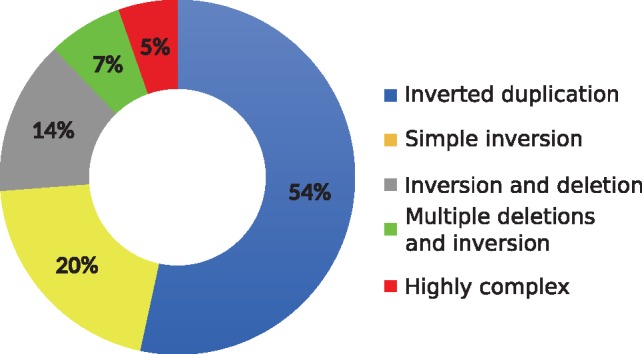
Relative abundance of complex SVs among the inversion calls reported in the 1000 Genomes Project (Sudmant et al., 2015). 54% of predicted inversions are in fact inverted duplications and only 20% are correctly predicted as simple inversions
Fig. 2.
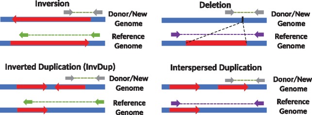
Read pair sequence signatures of inversions, deletions and segmental duplications. The gray arrows show read pairs that span a structural variant breakpoint, and green (left panel) and purple (right panel) arrows show the corresponding map location and orientation of these reads on the reference genome. Note that the read pair signatures for inversions and inverted duplications are exactly the same. Similarly, deletions and direct duplications show the same read pair signature. Therefore read pair based algorithms may incorrectly identify inverted segmental duplications as simple inversions. This problem also exists for incorrectly predicting simple deletions while the true underlying variant is duplication in direct orientation
2.2 Read pair and split read clustering
TARDIS uses a combination of read pair, read depth and split read sequencing signatures to discover SVs (Soylev et al., 2017). TARDIS formulation is based on algorithms we developed earlier using maximum parsimony (Hormozdiari et al., 2009, 2011b) objective function. The proposed approach has two main steps: First clustering read pairs and split reads that signal each specific type of SV, and second apply a strategy to select a subset of clusters as predicted SV. In this paper we extend TARDIS to characterize a complex set of SVs, which are incorrectly categorized by state-of-the-art methods for SV discovery. Specifically the methods we present here will advance our capability in discovery of duplication based SVs. Furthermore, our new methods are capable of separating inversions from more complex events of inverted duplications and are also able to predict the insertion locations of the new copies of SDs. We would argue that considering these more complex types of SV is crucial in improving the accuracy of predicting other types of SVs. We therefore modified TARDIS to calculate a likelihood score for each SV provided the observed read pair, read depth and split read signatures. Figure 3 summarizes the read pair signatures that TARDIS uses to find tandem in direct orientation and interspersed duplications in both direct and inverted orientation. Although not shown on the figure for simplicity, similar rules are required for split reads that signal the same types of SVs (Supplementary Fig. S1).
Fig. 3.
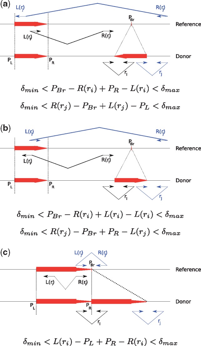
Read pair sequence signatures used in TARDIS to characterize (a) interspersed duplications in inverted orientation, (b) interspersed duplications in direct orientation and (c) tandem duplications. PBr denotes the breakpoint location of each variant, and PL and PR are the left and right (i.e. proximal and distal) coordinates of the duplicated segment. For each type of structural variation, we show two read pairs from the donor genome (ri, rj). The read pairs are colored black and blue to facilitate easier tracking by the reader. The alignments for read pair ri are shown on the reference as L(ri) and R(ri), which denote the left (i.e. proximal) and right (i.e. distal) mapping locations of the end reads. Finally, δmin and δmax are the minimum and maximum fragment lengths as inferred from the fragment size distribution in the aligned data
2.2.1. Maximal valid clusters
Our approach for discovery of SVs is based on first produced maximal valid clusters for every type of SVs. We have previously described algorithms to calculate maximal valid clusters for deletions, inversions and mobile element insertions (Hormozdiari et al., 2009, 2011a, b; Soylev et al., 2017). A valid cluster is defined as a set of discordant paired-end read alignments that support the same structural variants. In another words, a valid cluster indicates the set of discordant paired-end read mappings that explain the same potential structural variant. More formally, a valid cluster is a set of alignments of discordant read pairs and/or split reads (denoted as rpi) that support the same particular SV event shown as:
A maximal valid cluster is a valid cluster with no additional discordant paired-end reads can be added to it such that it still remains a valid cluster. Note that, we and others have previously developed methods to efficiently generate all maximal clusters for inversions, deletions and insertions. In this section we provide new methods to find maximum valid clusters for tandem and interspersed (both direct and inverted) duplications.
There are a set of rules that each rpi should satisfy in order to support the cluster, VClusi, based on the type of SV.
Inverted duplications: We assume the fragment sizes for read pairs are in the range [δmin, δmax], and we denote the insertion breakpoint of the duplication as PBr and the locus of the duplicated sequence is [PL, PR] (Fig. 3a). We scan the genome from beginning to end, and we consider each position as a potential duplication insertion breakpoint PBr. We consider all sets of read pairs where both mates map to the same strand (i.e. +/+ and −/−) within interval [PBr − δmax, PBr] and [PBr, PBr + δmax] respectively as clusters that potentially signal an inverted duplication.
Interspersed direct duplications: We create the valid clusters in a way similar to the inverted duplications, with the exception of the required read mapping properties. For direct duplications we require each mate of a read pair to map to opposing strands (i.e. +/− and −/+).
Tandem duplications: We also create the clusters for tandem duplications as shown in Figure 3. In the case of tandem duplications, discordant read pairs and split reads map in opposing strands, where the read mapping to the upstream location will map to the reverse strand, and the read mapping to downstream will map to the forward strand (i.e. −/+).
Similar to the valid cluster formulation, a maximal valid cluster is a valid cluster that encompasses all the valid read pairs and split reads for the particular SV event (i.e. no valid superset exists). This can be computed in polynomial time as follows:
We initially create maximal sets S = {S1, S2, …, Sk} that harbors the read pair/split read alignments .
For interspersed duplications, we use an additional step to bring mappings in both forward–reverse and reverse–forward (forward–forward and reverse–reverse for inverted duplications) orientations together inside the same set.
For each maximal overlapping set Si found in Step 1, we create all the overlapping maximal subsets si. (This step is necessary only for detecting inversions and interspersed duplications.)
Among all the sets si found in Step 3, remove any set that is a proper subset of another chosen set.
2.3 Probabilistic model
As we describe above different types of SVs may generate similar discordant read pair signatures (Fig. 2). We therefore developed a probabilistic model that makes use of the read depth signature to assign a likelihood score to each potential SV. Our new probabilistic model has the ability to distinguish different types of SVs with the same read pair signature.
2.3.1. Likelihood model
Assume the set of maximum valid clusters is observed in the sequenced sample. TARDIS keeps track the following information for each maximum valid cluster Si for :
Observed read depth and read pair information (di, pi), i.e. di is the total observed read depth, and pi is the number of discordantly mapped read pairs.
Potential duplicated or deleted or inverted region (αi, βi).
Potential breakpoint γi.
Potential SV type.
Assuming observed read depth and number of discordant read pairs follow a Poisson distribution, λ > 0,
here, λ is the expected number of read depth or read pairs, and x is the observed number of read depth or read pairs, respectively. However, the expected read depth or read pairs for some events might be zero, we approximate the probability by,
for a small ε > 0 (e.g. ε = 0.01 for read depth and ε = 0.001 for read pairs).
For each cluster Si, we define a random variable in which the state of Si is homozygous if statei = 2, heterozygous if statei = 1, and no event if statei = 0. We also define a random variable typei, which represents the SV type for Si. Given statei = k and typei = δ, the likelihood of Si can be calculated as:
where λd is the expected read depth of Si given and λp is the expected read pairs of Si given .
We calculate λd based on (typei, statei) and the expected read depth within the region (αi, βi) normalized with respect to its G + C content using a sliding window of size 100 bp, denoted by . We calculate λp based on the (typei, statei) and the expected number of discordantly mapped read pairs around the potential breakpoint γi, denoted by Ep[γi]. For instance, if an event is categorized as homozygous deletion, we expect to see almost no read depth inside the potential deleted region (αi, βi), and the expected number of discordantly mapped read pairs should be approximately the expected number of reads containing the potential breakpoint, i.e Ep[γj]. For heterozygous deletion events, we expect to see half of the number of read depths and half of the expected number of discordantly mapped read pairs. We also calculate the likelihood score of no event at the potential region given that is categorized as deletion. For this case, we expect to see the expected number of read depths in that potential region and zero discordantly mapped read pairs. Similarly, the value for λd, λp can be approximately for inversion and duplications. Table 1 shows the value for λd, λp for each (typei, statei) using and . Note that even though the formulation for λd, λp are the same for all types of duplications, the likelihood score will be different because the potential regions (αi, βi) are different based on the categorized type of the event being considered. Furthermore, the read pair support and signature will be different for each type of duplication which is the key in resolving the type of duplication.
Table 1.
Formulation for λd and λp for maximum valid cluster Si
| SV type | State | λd | λp |
|---|---|---|---|
| Deletion | Homozygous | 0.01 | |
| Heterozygous | |||
| No event | 0.001 | ||
| Inversion | Homozygous | ||
| Heterozygous | |||
| No event | 0.001 | ||
| Inverted duplication | Homozygous | ||
| Heterozygous | |||
| No event | 0.001 | ||
| Direct duplication | Homozygous | ||
| Heterozygous | |||
| No event | 0.001 | ||
| Tandem duplication | Homozygous | ||
| Heterozygous | |||
| No event | 0.001 |
2.3.2. SV weight
For each potential SV we calculate a score to represent how likely a SV prediction is correct given the observed signature. Note that, for each SV, we calculate the likelihood considering homozygous state and heterozygous state separately.
We define the score as ratio of log of likelihoods of the putative SV being true given the observed data over it being false. Note that we use log function to avoid numerical errors. Even though the standard approach is to use logarithm of the ratio, we heuristically use the ratio to make sure that the scores are positive, which will work better for the set cover approximation algorithm we will use in the next step.
The score of potential SV Si is defined as follows:
where δi is the potential SV type of Si. Again, k = 0, 1, 2 implies that the state of Si is no event, heterozygous and homozygous, respectively.
2.3.3. Multi-mapping reads
We have previously showed that a greedy approach motivated by weighted-set cover problem performs well in discovery of SVs with multiple mapping of the reads (Hormozdiari et al., 2009). It guaranties an O(log(n)) approximation. We therefore utilize a similar iterative greedy approach here as minimum weighted-set cover. More formally, at each step we select the set with the lowest ratio of SV score (score(Si)) and number of uncovered discordant paired-end reads being covered by that SV (pi)
and continues this iterative process.
3 Results
3.1 Simulation
In order to evaluate performance of our SV detection algorithms, we generated a simulated genome first using VarSim (Mu et al., 2015). VarSim ‘inserts’ previously known real genomic variants into a given reference segment. Although it supports deletions, inversions and tandem duplications, it does not yet simulate interspersed SDs. Therefore we developed a new simulator called CNVSim to additionally simulate interspersed duplications in both direct and inverted duplication.
In total, we simulated SVs of lengths selected uniformly random between 500 bp and 10 kb. For inverted duplications and interspersed direct duplications, the distance from the new paralog to the original copy is chosen uniformly random between 5000 bp and 50 kb. All segments are sampled randomly from the well-defined (i.e. no assembly gaps) regions in the reference genome, and guaranteed to be non-overlapping. Each simulated SV can be in homozygous or heterozygous state.
Based on the human reference genome (GRCh37), we simulated total of 1200 SVs including 700 deletions, 579 inversions, 200 tandem duplications, 200 inverted duplications and 200 interspersed direct duplications. We then simulated WGS data at four depths of coverages 10×, 20×, 30×, 60× using wgsim (https://github.com/lh3/wgsim). We mapped the reads back to the human reference genome (GRCh37) using BWA-MEM (Li, 2013). Finally we obtained SV call sets using TARDIS, DELLY (Rausch et al., 2012), LUMPY (Layer et al., 2014), TIDDIT (Eisfeldt et al., 2017), SVelter (Zhao et al., 2016) and SoftSV (Bartenhagen and Dugas, 2016).
We included analysis of all types of SVs in our simulation and real data experiments following our motivation we outlined in Section 2.1 and Figures 1 and 2. We would like to reiterate that inability to call interspersed SDs results in higher false positives in both deletion and inversion discovery. Through characterization of SDs and integration of a read depth based probabilistic model, TARDIS achieves better inversion and deletion discovery accuracy by correct classification of more complex SV types. Further analysis on the simulations revealed that 95 of 773 deletions predicted by LUMPY and 96 of 852 deletions predicted by DELLY are indeed interspersed duplications in direct orientation. Similarly, 109 of 1286 DELLY-predicted inversions were in fact inverted SDs.
Finally, we simulated 10 large (up to 1 Mbp) SDs in chromosome Y to assess the power of TARDIS in detecting large duplications. TARDIS correctly identified 4/10 duplications of size >63 kb (Supplementary Table S1).
Table 2 shows the true positive rate (TPR) and FDR of TARDIS compared to DELLY, LUMPY, TIDDIT, SVelter and SoftSV on the simulated data. TARDIS achieved a substantially higher TPR and a lower FDR for deletions and duplications overall. Additionally, its sensitivity is comparable to LUMPY and SoftSV in terms of inversion predictions (see Supplementary Fig. S2 for precision–recall curves of inversions and duplications).
Table 2.
Summary of simulation predictions by TARDIS, TIDDIT, LUMPY, SoftSV, DELLY and SVelter
| SV type | Cov. | TARDIS |
TIDDIT |
LUMPY |
SoftSV |
DELLY |
SVelter |
||||||||||||
|---|---|---|---|---|---|---|---|---|---|---|---|---|---|---|---|---|---|---|---|
| MISS | FDR | TPR | MISS | FDR | TPR | MISS | FDR | TPR | MISS | FDR | TPR | MISS | FDR | TPR | MISS | FDR | TPR | ||
| Deletion | 10× | 244 | 0.00 | 0.65 | 288 | 0.00 | 0.59 | 205 | 0.26 | 0.71 | 272 | 0.30 | 0.61 | 255 | 0.28 | 0.64 | 318 | 0.19 | 0.54 |
| 20× | 113 | 0.00 | 0.84 | 226 | 0.00 | 0.68 | 125 | 0.25 | 0.82 | 135 | 0.32 | 0.81 | 124 | 0.27 | 0.82 | 226 | 0.12 | 0.67 | |
| 30× | 92 | 0.00 | 0.87 | 194 | 0.00 | 0.72 | 111 | 0.24 | 0.84 | 109 | 0.32 | 0.84 | 106 | 0.30 | 0.85 | 188 | 0.11 | 0.73 | |
| 60× | 76 | 0.01 | 0.89 | 185 | 0.00 | 0.74 | 96 | 0.24 | 0.86 | 97 | 0.33 | 0.86 | 99 | 0.31 | 0.86 | 211 | 0.13 | 0.69 | |
| Inversion | 10× | 108 | 0.03 | 0.81 | 119 | 0.45 | 0.79 | 121 | 0.00 | 0.79 | 121 | 0.00 | 0.79 | 140 | 0.41 | 0.76 | 253 | 0.02 | 0.56 |
| 20× | 98 | 0.06 | 0.83 | 97 | 0.44 | 0.83 | 102 | 0.01 | 0.82 | 77 | 0.03 | 0.87 | 94 | 0.41 | 0.84 | 210 | 0.02 | 0.63 | |
| 30× | 88 | 0.06 | 0.85 | 101 | 0.44 | 0.83 | 98 | 0.01 | 0.83 | 65 | 0.03 | 0.89 | 87 | 0.43 | 0.85 | 205 | 0.03 | 0.64 | |
| 60× | 83 | 0.06 | 0.86 | 96 | 0.44 | 0.83 | 93 | 0.01 | 0.84 | 78 | 0.05 | 0.87 | 84 | 0.43 | 0.85 | 180 | 0.18 | 0.68 | |
| Duplication | 10× | 72 | 0.05 | 0.88 | 428 | 0.10 | 0.29 | 428 | 0.49 | 0.29 | 444 | 0.55 | 0.26 | 433 | 0.48 | 0.28 | 307 | 0.32 | 0.46 |
| 20× | 28 | 0.05 | 0.95 | 422 | 0.09 | 0.30 | 412 | 0.50 | 0.31 | 410 | 0.55 | 0.32 | 429 | 0.50 | 0.29 | 259 | 0.20 | 0.55 | |
| 30× | 25 | 0.04 | 0.96 | 424 | 0.10 | 0.29 | 410 | 0.50 | 0.32 | 403 | 0.57 | 0.33 | 419 | 0.50 | 0.30 | 200 | 0.04 | 0.65 | |
| 60× | 19 | 0.09 | 0.97 | 422 | 0.08 | 0.30 | 408 | 0.50 | 0.32 | 401 | 0.60 | 0.33 | 414 | 0.50 | 0.31 | 194 | 0.18 | 0.65 | |
Note: We show the true positive rate/recall and false discovery rates (TPR and FDR) of TARDIS, TIDDIT, LUMPY, SoftSV, DELLY and SVelter at different depths of coverage from 10× to 60× for deletions (Del), inversions (Inv) and segmental duplications (Dup). Note that only TARDIS and SVelter can predict interspersed segmental duplications, therefore other tools miss such events. TARDIS consistently shows low FDR with comparable sensitivity. In our simulation, the length of each SV is generated uniformly random between 500 bp and 10 kb. Note that the bold values for FDR and TPR represent the best results among the five tools. Note, that most tools have comparable performance if we only simulated deletions and inversions as shown in Supplementary Figure S4.
In these simulation experiments we used the default variables, which require at least five read pairs that support the SV event. Although this cut-off works well, it contributes to higher number of false positives when the depth of coverage is high (Table 2). To demonstrate the effects of the values for this parameter, we repeated the experiment with varying minimum number of read pair support values. We confirmed that with higher values, we can reduce the FDR for high coverage genomes (Supplementary Table S2).
Furthermore, TARDIS can classify duplications into tandem, interspersed directed duplication and inverted duplication. However, DELLY, LUMPY, TIDDIT and SoftSV are not designed to characterize interspersed SDs, therefore we cannot provide comparisons. SVelter, on the other hand, is one of the first tools to address complex SV types and is able to classify duplications. However, it shows lower TPR and higher FDR compared to TARDIS (see Supplementary Fig. S3 for precision–recall curves of tandem and interspersed duplications for TARDIS and SVelter). Table 3 shows the TDR, FDR and the exact count of the number of True/False predictions for each type of SD.
Table 3.
Characterization of different types of segmental duplications using TARDIS on simulated data
| Duplication type | Coverage | # SVs | Missed | True | TPR | False | FDR |
|---|---|---|---|---|---|---|---|
| Inverted interspersed duplication | 10× | 200 | 15 | 185 | 0.93 | 7 | 0.04 |
| 20× | 200 | 10 | 190 | 0.95 | 11 | 0.05 | |
| 30× | 200 | 12 | 188 | 0.94 | 15 | 0.07 | |
| 60× | 200 | 9 | 191 | 0.96 | 33 | 0.15 | |
| Direct interspersed duplication | 10× | 200 | 10 | 190 | 0.95 | 3 | 0.02 |
| 20× | 200 | 7 | 193 | 0.97 | 0 | 0.00 | |
| 30× | 200 | 6 | 194 | 0.97 | 4 | 0.02 | |
| 60× | 200 | 5 | 195 | 0.98 | 9 | 0.04 | |
| Tandem duplication | 10× | 200 | 47 | 153 | 0.77 | 21 | 0.12 |
| 20× | 200 | 11 | 189 | 0.95 | 15 | 0.07 | |
| 30× | 200 | 7 | 193 | 0.97 | 10 | 0.05 | |
| 60× | 200 | 5 | 195 | 0.98 | 16 | 0.08 |
Note: This table shows the true positive rate (recall) and false discovery rate (TPR and FDR respectively) of TARDIS for each type of duplication.
We also extended our analysis excluding the duplicated regions in the simulated genomes. Most tools performed similarly in predicting deletions and inversions within these regions (Supplementary Fig. S4). In other words, if we only simulate deletion and inversion SVs, most of the tools we tested have comparable results. However, we also observed that including complex duplications to the simulation will result in increase of false prediction for all types of SVs for most tools. In fact, we confirm (at least in simulations) that ignoring complex duplication events can have significant impact on precision and recall of other types of SVs.
3.2 Haploid genome analyses
As the first experiment with real datasets, we downloaded short read HTS data generated from two haploid cell lines, namely CHM1 and CHM13 (Huddleston et al., 2014; Steinberg et al., 2014). We mapped the reads to human reference genome (GRCh37) using BWA-MEM (Li, 2013). We also obtained call sets generated with PacBio data from the same genomes (Chaisson et al., 2015b), but here we use updated SV calls (M. Chaisson, personal communication), which we use as the true inversion set to compare with our predictions.
We present the comparison of the inversion predictions made by TARDIS and two state-of-the-art methods LUMPY and DELLY in Figure 4. Note that we only consider inversions of length >100 bp. Figure 4a and b shows the comparison of TARDIS predictions with those of other tools on CHM1 and CHM13, respectively (we also present a similar comparison for deletion predictions in Supplementary Fig. S5). Overall, TARDIS achieves better accuracy. We also tested the highest scoring set (n = 50) of predicted inversions by each tool generated for the CHM1 genome. Briefly, we used a reference-guided de novo assembly of PacBio reads generated from the same genome (Chaisson et al., 2015b) and mapped the contigs to the loci of interest. We show a receiver-operating-characteristic-like plot that uses actual numbers of true and false calls instead of rates (TPR/FDR) (Supplementary Fig. S6). Here we observe that compared to LUMPY and DELLY, TARDIS achieves better area under the curve. However, we note that the main reason for DELLY and LUMPY curves being closer to that of TARDIS for low number of false calls is because there were several predictions for which corresponding contigs did not exist in the assembled genome, therefore omitted from this plot.
Fig. 4.
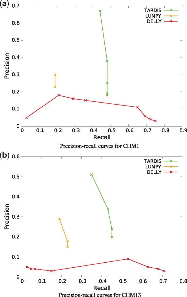
Precision–recall curves for the comparison of inversion predictions on (a) CHM1 and (b) CHM13 genomes, based on predicted inversions using BLASR mappings of PacBio reads
We provide the full set of the 50 highest scoring SDs that TARDIS predicts in the CHM1 genome together with in silico validation using the corresponding PacBio-based assembly (Supplementary Table S3). Almost all of the predicted duplications, except one, were validated using long reads. (We also provide the PacBio alignments of some of these events and top 20 highest scoring CHM13 predictions in Supplementary Table S4.) Note that in most cases TARDIS assigned the correct subtype of duplications (inverted, direct or tandem duplication) to the prediction. As expected, the highest number of SDs in the top 50 were tandem duplications (>50% of all duplications).
3.3 NA12878 genome
We also analyzed the WGS data generated from NA12878 using TARDIS for various types of SV discovery and compared the results against state-of-the-art methods for inversion prediction. Similar to the simulation and CHM1/13 results, TARDIS outperformed the tested methods for SV discovery (see Supplementary Fig. S18 for inversion comparison with a set of validated inversions on this sample).
More interestingly, we have found an example of a large inverted duplication in NA12878 sample which we validated using available orthogonal PacBio data generated from the same sample (Fig. 5). The interesting point about this inverted duplication is that it is larger than 10 kb and the distance between locus of insertion and the duplicated region is also larger, which shows a potential start of a new SD.
Fig. 5.

(a) Illumina read mapping information visualized using IGV (Thorvaldsdóttir et al., 2013). Here the read pairs in the NA12878 genome show typical inversion signature (red lines), where all reads map concordantly in CHM1 and CHM13 genomes, and a simple sketch of the alternative inverted duplication structure of the same region. (b) Dot plot matrix validation using PacBio data, which shows an inverted duplication. The whole genome assembly shows an inverted duplication of a 12 kb segment separated by 10 kb. This region demonstrates the case where read pair based clustering confuses an inverted duplication with a simple inversion
4 Discussion
Characterization of structural variants using HTS data is a well-studied problem. Still, due to the difficulty of accurately predicting complex variants, most of the current approaches mainly focus on specific forms of SVs. In this paper, we describe novel algorithms to detect complex SV events such as tandem, direct and inverted interspersed SDs simultaneously with simpler forms SV using whole genome sequencing data. Our approach integrates multiple sequence signatures to identify and cluster potential SV regions under the assumption of maximum parsimony. However, complex SV events usually generate similar signatures (i.e. inversion versus inverted duplication), which make it difficult to differentiate particular SV types. Therefore, we strengthened our method by using a probabilistic likelihood model to overcome this obstacle by calculating a likelihood score for each SV.
Using simulated and real datasets, we showed that TARDIS outperforms state-of-the-art methods in terms of specificity for all types of SVs, and achieves considerably high true discovery rate for SDs with moderate time and memory requirements (see Supplementary Table S5 for a comparison of different tools for CHM1 and NA12878 genomes). It should be noted that it TARDIS is currently one of the few methods that can classify duplications as tandem and interspersed in direct or inverted orientation using HTS data. Additionally, it demonstrates comparable sensitivity in deletions and inversions.
Here we only focused on tandem duplications in direct orientation, although inverted tandem repeats in genomes, or DNA palindromes, also exist especially in the human Y chromosome (Brand et al., 2015; Trombetta and Cruciani, 2017). However, these DNA palindromes were incorporated in the human genome over millions of years of evolution, and polymorphic inverted tandem duplication events are rare. Because of this, the mechanisms forming DNA palindromes are not yet well-established and we are not aware of a resource of validated DNA palindrome polymorphisms. We therefore ignore such variants in this study and we aim to address them in the future.
Future improvements in TARDIS will include addition of local assembly signature to help it achieve better accuracy. Although simulation experiments demonstrated potential efficacy of TARDIS in SD predictions, those that are generated from real genomes need to be experimentally verified to fully understand the power and shortcomings of the TARDIS algorithm. We can then apply TARDIS to thousands of genomes that were already sequenced as part of various projects, such as the 1000 Genomes Project to advance our understanding of the SV spectrum in human genomes. Another possible direction for TARDIS can be integration of new methods to better detect somatic SV detection, which we can then apply to cancer genomes.
Supplementary Material
Acknowledgements
We thank E. Ebren and F. Karaoglanoglu for their help in creating simulation datasets. We also thank E. E. Eichler for insightful advice and comments. Part of the work was done during F.H. postdoc training in E.E. Eichler’s lab. We would also like to thank M. Chaisson for providing PacBio call sets for CHM1 and CHM13, and also the local assembly of these genomes.
Funding
This work was supported by a grant by TÜBİTAK [215E172] and an EMBO Installation Grant [IG-2521 to C.A.] and an NSF grant [1528234 to T.L.]. The authors also acknowledge the Computational Genomics Summer Institute funded by NIH grant [GM112625] that fostered international collaboration among the groups involved in this project.
Availability
TARDIS is available under BSD 3-clause license at https://github.com/BilkentCompGen/tardis, and the CNVSim simulator is available at https://github.com/HormozdiariLab/CNVsim. Docker image for TARDIS is also available at https://hub.docker.com/r/alkanlab/tardis/.
NA12878 WGS dataset can be downloaded from https://www.illumina.com/platinumgenomes.html. SRA IDs for CHM1 and CHM13 are SRP044331 and SRP080317, respectively. GenBank assembly accession numbers for CHM1 and CHM13 assemblies are GCA_000306695.2 and GCA_000983455.2. We deposited current versions of TARDIS (1.0.2) and CNVSim, and all predictions, truth sets and the CRAM files for the simulation data to Zenodo (doi: 10.5281/zenodo.2611109).
Conflict of Interest: none declared.
References
- Abyzov A. et al. (2011) CNVnator: an approach to discover, genotype, and characterize typical and atypical CNVs from family and population genome sequencing. Genome Res., 21, 974–984. [DOI] [PMC free article] [PubMed] [Google Scholar]
- Alkan C. et al. (2009) Personalized copy number and segmental duplication maps using next-generation sequencing. Nat. Genet., 41, 1061–1067. [DOI] [PMC free article] [PubMed] [Google Scholar]
- Alkan C. et al. (2011) Genome structural variation discovery and genotyping. Nat. Rev. Genet., 12, 363–376. [DOI] [PMC free article] [PubMed] [Google Scholar]
- Bartenhagen C., Dugas M. (2016) Robust and exact structural variation detection with paired-end and soft-clipped alignments: SoftSV compared with eight algorithms. Brief. Bioinform., 17, 51–62. [DOI] [PubMed] [Google Scholar]
- Brand H. et al. (2015) Paired-duplication signatures mark cryptic inversions and other complex structural variation. Am. J. Hum. Genet., 97, 170–176. [DOI] [PMC free article] [PubMed] [Google Scholar]
- Chaisson M.J.P. et al. (2015a) Genetic variation and the de novo assembly of human genomes. Nat. Rev. Genet., 16, 627–640. [DOI] [PMC free article] [PubMed] [Google Scholar]
- Chaisson M.J.P. et al. (2015b) Resolving the complexity of the human genome using single-molecule sequencing. Nature, 517, 608–611. [DOI] [PMC free article] [PubMed] [Google Scholar]
- Chaisson M.J.P. et al. (2018) Multi-platform discovery of haplotype-resolved structural variation in human genomes. bioRxiv, 193144. [DOI] [PMC free article] [PubMed] [Google Scholar]
- Conrad D.F. et al. (2010) Origins and functional impact of copy number variation in the human genome. Nature, 464, 704–712. [DOI] [PMC free article] [PubMed] [Google Scholar]
- Cooper G.M. et al. (2008) Systematic assessment of copy number variant detection via genome-wide SNP genotyping. Nat. Genet., 40, 1199–1203. [DOI] [PMC free article] [PubMed] [Google Scholar]
- Eisfeldt J. et al. (2017) TIDDIT, an efficient and comprehensive structural variant caller for massive parallel sequencing data. F1000Res., 6, 664.. [DOI] [PMC free article] [PubMed] [Google Scholar]
- Hormozdiari F. et al. (2009) Combinatorial algorithms for structural variation detection in high-throughput sequenced genomes. Genome Res., 19, 1270–1278. [DOI] [PMC free article] [PubMed] [Google Scholar]
- Hormozdiari F. et al. (2011a) Alu repeat discovery and characterization within human genomes. Genome Res., 21, 840–849. [DOI] [PMC free article] [PubMed] [Google Scholar]
- Hormozdiari F. et al. (2011b) Simultaneous structural variation discovery among multiple paired-end sequenced genomes. Genome Res., 21, 2203–2212. [DOI] [PMC free article] [PubMed] [Google Scholar]
- Huddleston J. et al. (2014) Reconstructing complex regions of genomes using long-read sequencing technology. Genome Res., 24, 688–696. [DOI] [PMC free article] [PubMed] [Google Scholar]
- Huddleston J. et al. (2016) Discovery and genotyping of structural variation from long-read haploid genome sequence data. Genome Res., 27, 677–685. [DOI] [PMC free article] [PubMed] [Google Scholar]
- Iakovishina D. et al. (2016) SV-Bay: structural variant detection in cancer genomes using a Bayesian approach with correction for GC-content and read mappability. Bioinformatics, 32, 984–992. [DOI] [PMC free article] [PubMed] [Google Scholar]
- Korbel J.O. et al. (2007) Paired-end mapping reveals extensive structural variation in the human genome. Science, 318, 420–426. [DOI] [PMC free article] [PubMed] [Google Scholar]
- Layer R.M. et al. (2014) LUMPY: a probabilistic framework for structural variant discovery. Genome Biol., 15, R84.. [DOI] [PMC free article] [PubMed] [Google Scholar]
- Lee S. et al. (2009) MoDIL: detecting small indels from clone-end sequencing with mixtures of distributions. Nat. Methods, 6, 473–474. [DOI] [PubMed] [Google Scholar]
- Li H. (2013) Aligning sequence reads, clone sequences and assembly contigs with BWA-MEM. arXiv Preprint arXiv, 1303, 3997. [Google Scholar]
- Marth G.T. et al. (1999) A general approach to single-nucleotide polymorphism discovery. Nat. Genet., 23, 452–456. [DOI] [PubMed] [Google Scholar]
- McCarroll S.A. et al. (2006) Common deletion polymorphisms in the human genome. Nat. Genet., 38, 86–92. [DOI] [PubMed] [Google Scholar]
- Medvedev P., Brudno M. (2008) Ab initio whole genome shotgun assembly with mated short reads. In: Annual International Conference on Research in Computational Molecular Biology, Springer, Berlin, Heidelberg, pp. 50–64. [Google Scholar]
- Medvedev P. et al. (2009) Computational methods for discovering structural variation with next-generation sequencing. Nat. Methods, 6, S13–S20. [DOI] [PubMed] [Google Scholar]
- Mills R.E. et al. (2006) An initial map of insertion and deletion (INDEL) variation in the human genome. Genome Res., 16, 1182–1190. [DOI] [PMC free article] [PubMed] [Google Scholar]
- Mu J.C. et al. (2015) VarSim: a high-fidelity simulation and validation framework for high-throughput genome sequencing with cancer applications. Bioinformatics, 31, 1469–1471. [DOI] [PMC free article] [PubMed] [Google Scholar]
- Obe G. et al. (2002) Chromosomal aberrations: formation, identification and distribution. Mutat. Res., 504, 17–36. [DOI] [PubMed] [Google Scholar]
- Rausch T. et al. (2012) DELLY: structural variant discovery by integrated paired-end and split-read analysis. Bioinformatics, 28, i333–i339. [DOI] [PMC free article] [PubMed] [Google Scholar]
- Redon R. et al. (2006) Global variation in copy number in the human genome. Nature, 444, 444–454. [DOI] [PMC free article] [PubMed] [Google Scholar]
- Rowley J.D. (1973) A new consistent chromosomal abnormality in chronic myelogenous leukaemia identified by quinacrine fluorescence and giemsa staining. Nature, 243, 290–293. [DOI] [PubMed] [Google Scholar]
- Sebat J. et al. (2004) Large-scale copy number polymorphism in the human genome. Science, 305, 525–528. [DOI] [PubMed] [Google Scholar]
- Sharp A.J. et al. (2006) Discovery of previously unidentified genomic disorders from the duplication architecture of the human genome. Nat. Genet., 38, 1038–1042. [DOI] [PubMed] [Google Scholar]
- Shendure J., Ji H. (2008) Next-generation DNA sequencing. Nat. Biotechnol., 26, 1135–1145. [DOI] [PubMed] [Google Scholar]
- Sindi S. et al. (2009) A geometric approach for classification and comparison of structural variants. Bioinformatics, 25, i222–i230. [DOI] [PMC free article] [PubMed] [Google Scholar]
- Soylev A. et al. (2017) Toolkit for automated and rapid discovery of structural variants. Methods, 129, 3–7. [DOI] [PubMed] [Google Scholar]
- Steinberg K.M. et al. (2014) Single haplotype assembly of the human genome from a hydatidiform mole. Genome Res., 24, 2066–2076. [DOI] [PMC free article] [PubMed] [Google Scholar]
- Sudmant P.H. et al. (2010) Diversity of human copy number variation and multicopy genes. Science, 330, 641–646. [DOI] [PMC free article] [PubMed] [Google Scholar]
- Sudmant P.H. et al. (2015) Global diversity, population stratification, and selection of human copy-number variation. Science, 349, aab3761. [DOI] [PMC free article] [PubMed] [Google Scholar]
- The 1000 Genomes Project Consortium. (2015) A global reference for human genetic variation. Nature, 526, 68–74. [DOI] [PMC free article] [PubMed] [Google Scholar]
- Thorvaldsdóttir H. et al. (2013) Integrative genomics viewer (IGV): high-performance genomics data visualization and exploration. Brief. Bioinform., 14, 178–192. [DOI] [PMC free article] [PubMed] [Google Scholar]
- Trombetta B., Cruciani F. (2017) Y chromosome palindromes and gene conversion. Hum. Genet., 136, 605–619. [DOI] [PubMed] [Google Scholar]
- Tuzun E. et al. (2005) Fine-scale structural variation of the human genome. Nat. Genet., 37, 727–732. [DOI] [PubMed] [Google Scholar]
- Ye K. et al. (2009) Pindel: a pattern growth approach to detect break points of large deletions and medium sized insertions from paired-end short reads. Bioinformatics, 25, 2865–2871. [DOI] [PMC free article] [PubMed] [Google Scholar]
- Zhao X. et al. (2016) Resolving complex structural genomic rearrangements using a randomized approach. Genome Biol., 17, 126. [DOI] [PMC free article] [PubMed] [Google Scholar]
Associated Data
This section collects any data citations, data availability statements, or supplementary materials included in this article.