Spatial Firing Properties of Hippocampal CA1 Populations in an Environment Containing Two Visually Identical Regions

Abstract

Populations of 10-39 CA1 pyramidal cells were recorded from four rats foraging for food reward in an environment consisting of two nearly identical boxes connected by a corridor. For each rat, a higher-than-chance fraction of cells had similarly shaped spatial firing fields in both boxes, but other cells had completely different fields in the two boxes. The level of correlation of fields in the two boxes differed greatly across rats and, for three of the four rats, across recording sessions. Thus, the factors controlling the level of correlation are likely to be subtle. Two control manipulations were performed. First, the two boxes were physically interchanged. In no case did firing fields move along with the boxes. Second, on the final session of recording, the rat was started in the south box, after having been started in the north box for every previous session. For at least two of the four rats, the north fields from the previous session were instantiated in the south during the first visit of the second session, but thereafter reverted. Thus neither differences between the physical boxes nor sensory input from outside the apparatus could account for the differences in firing fields: most likely they were caused by a combination of learned expectations and a neural mechanism for remembering movements. These findings could be explained either by hypothesizing a more sophisticated attractor-map architecture than has been proposed previously, or by hypothesizing that the hippocampus conjunctively encodes both map information and some other type of information.

In many situations, pyramidal cells in the rat hippocampus display place-dependent activity. A typical cell will fire robustly whenever the rat enters a particular small portion of the environment, and be virtually silent at other times. When multiple cells are examined together, their place fields distribute, in apparently a random way, across the entire environment. These findings have provoked the idea that hippocampal population activity constitutes a “cognitive map” of the animal’s spatial location (O’Keefe and Nadel, 1978). An extensive body of research over the past two decades has aimed at defining the properties of these maps and the neural mechanisms that give rise to them. [For pointers to the literature, see McNaughton et al. (1996) and Wiener (1996).]

The most straightforward hypothesis would be that a cell fires when the animal is in a given place because it is sensitive to some specific combination of sensory features—for example, the visual angle between two landmarks (Zipser, 1985; McNaughton et al., 1991). It has gradually become clear, however, that this type of explanation cannot be correct. Switching off the lights while an animal is inside an environment does not disrupt spatial firing, nor does removal of other sensory modalities such as audition or olfaction. Only complete disorientation, or strong cue-conflict, is capable of shifting place fields. Moreover, the effects of cue-conflict are sometimes delayed, indicating that the mapping system has an intrinsic dynamic stability (Gothard et al., 1996). Also, bringing an animal twice into the same environment to perform the same task can sometimes lead to the instantiation of different, and apparently unrelated, hippocampal maps on the two occasions (Barnes et al., 1997). To account for these properties, it has been proposed that cognitive maps are stored as sets of dynamical attractors inside the hippocampal formation, and that the primary mechanism for shifting the internally represented spatial location is the animal’s integration of its own movements (a process generally called “path integration”), with learned sensory relationships coming into play as a secondary calibrating factor (McNaughton et al., 1996; Samsonovich and McNaughton, 1997). On the basis of the available evidence from the literature indicating that hippocampal maps may be uncorrelated even for visually similar environments (Quirk et al., 1992), Samsonovich and McNaughton (1997) made the assumption that the hippocampal maps instantiated in any two situations either should be identical or completely “orthogonal” (i.e., statistically unrelated). In other words, if the hippocampus encodes pure spatial coordinates, and the animal is “aware” that two environments, although visually identical, are in fact different places, then the hippocampal codes for the two environments should be orthogonal.

The experiment reported here was designed to examine the ability of the hippocampus to form orthogonal representations of similar situations, by using an environment containing two interconnected regions that were made as nearly as possible identical. It was expected that the hippocampal maps in the two regions would turn out to be completely orthogonal, or if not, to be essentially identical. As it turned out, the data did not accord with either prediction. The hippocampal maps for the two identical regions were neither identical nor orthogonal but rather partially overlapping. Furthermore, there were large and reliable differences between individual subjects in the degree of relatedness of the two maps. This article presents these findings and discusses their theoretical significance.

MATERIALS AND METHODS

The surgical and electrophysiological techniques used in this experiment have been described in detail in previous publications (Skaggs et al., 1996). Briefly, male Fischer–Brown Norway hybrid rats (Harlan Sprague Dawley), ∼9 months old, were implanted stereotaxically, under Nembutal anesthesia, with chronic recording microdrive arrays. Each array contained 14 independently adjustable microdrives loaded with four-channel “tetrodes.” Twelve of the tetrodes were aimed at the CA1 cell body layer and used for unit recording; one was positioned in the corpus callosum above the hippocampus and used as a reference for differential recording, and the final electrode was positioned near the level of the hippocampal fissure and used to record EEG. The tetrodes were arranged in a hexagonal lattice roughly 2 mm in diameter, and the center of the array was positioned at coordinates 3.7 mm posterior, 2.0 mm lateral from bregma. After recovery from surgery, the unit-recording tetrodes were lowered gradually, over the course of several days, to the CA1 cell body layer, which was recognized by standard electrophysiological criteria. Under ideal conditions, a tetrode placed in the CA1 cell body layer can pick up distinguishable signals from as many as 20 pyramidal cells, which can be isolated from each other using a “stereo” principle based on the relative spike sizes on different channels of the tetrode (McNaughton et al., 1983; O’Keefe and Recce, 1993). Thus, in principle, an array of 12 tetrodes can yield well over 100 distinguishable pyramidal cells, but yields of 40–60 are more commonly achieved. In this experiment, only cells that showed recognizable activity inside the experimental apparatus were considered. Previous studies have shown that in most cases approximately two-thirds of hippocampal pyramidal cells are silent in a given behavioral paradigm; these cells can be recognized by recording during slow-wave sleep (Thompson and Best, 1989). Pyramidal cells were distinguished from interneurons on the basis of spike waveforms and statistical properties of the spike train; only units classified as pyramidal cells were used in the data analysis.

For recording, a headstage was attached to the drive array, which was connected to a cable leading to a commutator mounted in the ceiling of the recording area. The headstage contained two sets of light-emitting diodes, enabling position and head direction to be tracked using a video camera, which also was mounted in the ceiling of the recording room. Data acquisition was performed using eight 80486-based microcomputers, running DataWave Discovery software (Longmont, CO) with synchronized timestamp clocks. After each day’s recording, the data were transferred to Sun workstations for processing and analysis.

Apparatus and training procedure

The behavioral apparatus was designed to permit a rat to travel between two regions that were as nearly as possible identical, both visually and in terms of behavioral demands. It was also considered important to ensure that the two regions were identically oriented and to avoid disorienting the rats rotationally, so that the sense of direction could not be used to distinguish the regions. The behavioral protocol was designed to motivate the rats to move back and forth between the two regions and repeatedly visit every part of each region.

The rats were initially placed on a restricted-feeding regimen, and after their weights had dropped to ∼80% of baseline, they were pretrained to forage for randomly scattered chocolate sprinkles inside a 67 × 67 cm plywood box placed on a table at the center of a room. Other than being square and opaque, this pretraining box had no visual resemblance to the apparatus used in the actual experiment. After recovery from surgery, the rats were given several more days of pretraining, with the recording headstage and cable attached. This was done to accustom the rats to the recording hardware and maximize the likelihood that they would perform well the first time they were introduced into the experimental apparatus.

The experimental apparatus consisted of two 58 × 61 cm wide by 61 cm high plywood boxes, painted flat gray, connected to each other by a corridor (Fig. 1). The intent was that the two boxes would be as nearly as possible visually identical. In each box a trapezoidal doorway 4 cm wide at the bottom, broadening to 46 cm at the top, was cut in the center of one wall. A thin metal strip, used to improve the rigidity of the boxes, ran across the floor of each doorway. Small battery-powered incandescent lights were mounted at the center of the walls opposite the doorways, 54 cm above the floor of the box. The lights were shielded by cut-out film canisters so that the only illumination came through small rectangular holes, directed downward toward the floor. Translucent white tape was placed over the holes to reduce the light and prevent the formation of sharp shadows. The boxes were open on the bottom, and the floor beneath them was covered with brown wrapping paper, which was changed between recording sessions, as described below. The apparatus was placed in a sound-attenuated room with black walls, and the only light came from the lights inside the maze. There was enough light in the room for a human experimenter to see very dimly, but for a rat inside one of the boxes, with the light shining down into his eyes, it is unlikely that anything outside was visible.

Fig. 1.

Apparatus for the experiment. A, Floor plan. The two boxes and corridor wall were all separate pieces, which could be disassembled to exchange the boxes between sessions of an experiment. Small downward-facing lights were mounted in the middle of each wall opposite the doorways. B, Photograph of the apparatus and the recording area in which it was located.

The boxes were constructed so that the two of them, and a separate piece forming the outer wall of the corridor, were held together by a set of easily removable metal clips. It took 5–10 min to disassemble the apparatus, move the boxes off to the side, replace the paper on the floor, move the boxes back into position, and reconnect them. The two boxes were marked with letters “A” and “B.” Some sessions were run with box A in the north (N) position and B in the south (S); others were run with the two boxes reversed, as described in more detail below.

During the first few days of recording, only a single session was conducted per day, lasting as long as the rat would continue to search for food. Once the duration approached 30 min (usually after 3–4 d), the protocol was changed to two 12–15 min sessions per day, with the floor paper replaced and boxes interchanged between sessions. The rat was conveyed to and from the apparatus inside a small cardboard box, nearly closed on top. Before and after the recording sessions, and while the boxes were being interchanged, the rat was held in a large cardboard box on a table ∼5 feet east of the recording area. At the beginning of each session the rat was picked up, placed inside the transfer box, and carried to the two-box apparatus by one of the experimenters, who in the process made a series of slow north-south translational movements, to prevent the rat from determining his starting location by integrating his motion with respect to the holding box. Because it was considered important not to disrupt the rat’s sense of direction, the experimenter made an effort only to translate the transfer box, not to rotate it. The transfer box was then placed on the floor of the recording area, and the rat was released. In every case but one, the rat was started on the N side of the two-box apparatus. This was true both when there was one session and when there were two sessions in a day, with the sole exception of the final day of recording (described below). The physical box (A or B) that was initially located on the N side was alternated from day to day. When two sessions were conducted, the A and B boxes were exchanged between sessions.

An assistant was inside the room with the rat while the recording sessions were conducted, and the experimenter was in an adjoining room monitoring the computers, occasionally giving instructions over an intercom. Before the rat was initially released, a small handful of chocolate sprinkles was scattered diffusely across the N box. The assistant in the room mentally divided the box into a 3 × 3 grid, and the rat was required, in the judgement of the assistant, to visit every sector, at which time she scattered food on the opposite side. The purpose of this was to ensure that the rat would spend a substantial amount of time, and sample each part of the box, on each visit. Except during the initial period in the N box, the rat was free at all times to pass through the corridor at will, but no additional food was dropped until he had visited every ninth part of the currently active box. The sound of chocolate sprinkles dropping on paper was easily audible and usually caused the rat to run immediately to the opposite box. During the recording session, the assistant inside the room supported the recording cable by hand, as nearly as possible directly above the rat, so that the pull of the cable would not provide a directional cue to distinguish between the N and S boxes. The cable was always kept slack, so that the motions of the rat would not be guided by the assistant. The assistant wore dark clothing and shifted her position north–southward in a quasi-random way along the west side of the apparatus so that she did not provide a reliable distinguishing cue. In any case, with the box lights in between shining down into their eyes, it was unlikely that the rats could see her, and they gave no obvious sign of being aware of her presence, except at the end of a session when she moved around to the east side of the apparatus to pick them up.

The first rat of the group quickly developed a habit of running immediately through the corridor to the S box. Because this would interfere with the test planned for the final day of recording, a small modification was made in the procedure, beginning on the sixth day: a brick was initially placed in the doorway, to prevent the rat from passing through it. After the rat had spent ∼1 min inside the N box, the brick was removed; all subsequent sessions for this rat were conducted this way. Rat 2, however, when treated the same way, climbed over the brick, so it was replaced on his fifth day with a large white cylindrical plastic jar, and all subsequent sessions for this rat and the remaining two rats were conducted this way. The brick or jar were present only during the first visit to the initial box. For the remainder of the session, the rat was free to move at will between boxes. Removing the brick or jar from the doorway caused no apparent changes in the pattern of hippocampal cell activity.

On the final day of recording, a special probe session was conducted. The first session of the day was conducted as usual; the boxes were disassembled and the floor paper was replaced, but then, contrary to the previous procedure, the boxes were reassembled in the same locations they had occupied during the first session. During the second (probe) session, the rat was placed initially on the S side of the apparatus, rather than being placed initially on the N side as in every previous session. In every other respect, the procedure for the probe session was as usual.

Data analysis

Correlation analysis. A major part of the analysis consisted of interpreting correlations between firing rate maps. For this purpose, a 64 × 64 pixel firing rate map was first calculated for the entire environment, and then 14 × 14 pixel portions were extracted for the regions corresponding to the N and S boxes. These sub-maps could then be compared using Pearson correlation coefficients. Pixels having zero occupancy in either box (and hence an undefined firing rate) were omitted from the calculation (these were rare). Because correlation coefficients become very noisy when firing rates are very low, for most analyses the cells were required to have spatial firing rates exceeding 1 Hz at some point in both boxes to be included.

The 64 × 64 pixel firing rate maps were constructed using an “adaptive smoothing” method that has been described in previous publications (Skaggs et al., 1996). Briefly, the method is designed to optimize the tradeoff between blurring error (attributable to averaging together data from locations with different true firing rates) and sampling error (the statistical error attributable to the limited number of samples available). To calculate the firing rate at a given point, a circle centered on the point is gradually expanded until the following criterion is met:

$$r\ge \frac{\alpha }{n\sqrt{s}},$$ Equation 1

where α is a constant, r is the radius of the circle in pixels, n is the number of 50-msec-long occupancy samples lying within the circle, and s is the total number of spikes contained in those occupancy samples. Once this criterion was met, the firing rate assigned to the point was equal to s/n. For this experiment, α was set to the value 1000.

In data sets composed of a single session, correlations between the north and south firing fields (denoted N–S) were calculated for each pyramidal cell. When there were two sessions, six types of correlation could be calculated, denoted N1–N2, N1–S1, N1–S2, S1–N2, S1–S2, and S1–S2, where for example N1–S2 is the correlation between the north firing rate map during session 1 and the south firing rate map during session 2. For the probe session (in which the rat was introduced to the apparatus inside the S box for the first time), two special firing rate maps were calculated, denoted S2a (representing the first period of time in the S box in session 2, lasting ∼2 min) and S2b (representing all remaining visits to the S box in session 2).

Comparisons of correlation distributions were performed using either factorial ANOVAs, the nonparametric Kolmogorov–Smirnov test (Press et al., 1992), or, for comparison of means, Student’s ttest.

Trajectory reconstruction. To analyze the moment-to-moment dynamics of population activity, a Bayesian method of trajectory reconstruction was used, as described by Zhang et al. (1998). This method makes use of firing rate maps to infer the most likely location of the rat from a brief sample of population activity and has been shown to perform better than a number of other reconstruction techniques. For the current experiment, the method was used only where data from two consecutive sessions were available: firing rate maps constructed from the first session were used to reconstruct trajectories during the second session. Briefly, a 64 × 64 pixel firing rate map was constructed for each pyramidal cell, as described above, using data from the first session. The second session was split into 1 sec intervals, and the number of spikes fired by each cell in the population was counted for each interval. On the basis of these spike counts, a probability was assigned to each location in the environment using the Poisson-distribution-based formula:

$$P(x)=\prod _i\frac{[{\lambda }_i(x){]}^{n_i}{e}^{-{\lambda }_i(x)}}{n_i!},$$ Equation 2

where i indexes the cells in the population, n_i is the number of spikes emitted by cell i, and λ_i(x) is the firing rate of cell i at location x. The reconstructed location was then the value of x that made P(x) maximal. To reduce the level of noise, each sample was required to have at least three active cells, and at least 10 total spikes, to be included.

This technique was called the “Bayesian one-step” method by Zhang et al. (1998). They also described a “Bayesian two-step” method that produced more accurate reconstructions, but it relies on a continuity constraint that would defeat the purpose for which the analysis was used in the current experiment.

RESULTS

Data were obtained from four rats, beginning with the first experience of each in the two-box environment. Rat 3, however, refused to leave the starting (N) box during his first session. In his second session, he went three times into the corridor but refused to enter the S box. To encourage him to run, the next two sessions were conducted without the recording headstage and cable attached; thus no data were taken. Thereafter this rat proved to be comfortable enough for the standard procedure to be followed. The other three rats moved back and forth between the N and S boxes during the first session and all subsequent sessions. The total number of recording days ranged from 9 to 12, and the number of usable cells per session ranged from 10 (worst session for rat 4) to 39 (best session for rat 1). Because there were clear individual differences between rats in the firing properties of cells (described below), data from each rat were analyzed separately. Data from four recording sessions were lost because of computer problems.

During the first few sessions, the behavior of the rats was erratic. They would often leave a box after exploring only a portion of it. Because no food was scattered on the opposite side until every ninth part of the current box had been visited, the rats eventually learned to scour the box in a more or less systematic way before leaving, although they never became completely reliable about this. During the first recording session, the number of corridor transits ranged from 7 (rat 1) to 12 (rat 2), with the exception of rat 3, who never left the N box at all. The initial time spent in the N box before first leaving it ranged from 2 min 25 sec (rat 2) to 9 min 55 sec (rat 1), again excluding rat 3.

Figures 2 and3 illustrate, for rats 1 and 2, the spatial firing fields of 25 simultaneously recorded CA1 pyramidal cells, in the first and second recording sessions of a single day. Between sessions, the two physical boxes were interchanged. For rat 1 (Fig. 2), most firing fields were completely different in the N and S boxes, but there were a few cases of similar fields. For rat 2 (Fig.3), in contrast, most fields were similar on both sides, but there were a few cases of strong difference, and most of these were maintained across both sessions. Rats 3 and 4, in common with rat 2, showed a majority of cells with symmetrical N–S fields, although the proportion was not quite as large as for rat 2. As described quantitatively below, this pattern of individual differences between rats was maintained reliably over the entire course of recording.

Fig. 2.

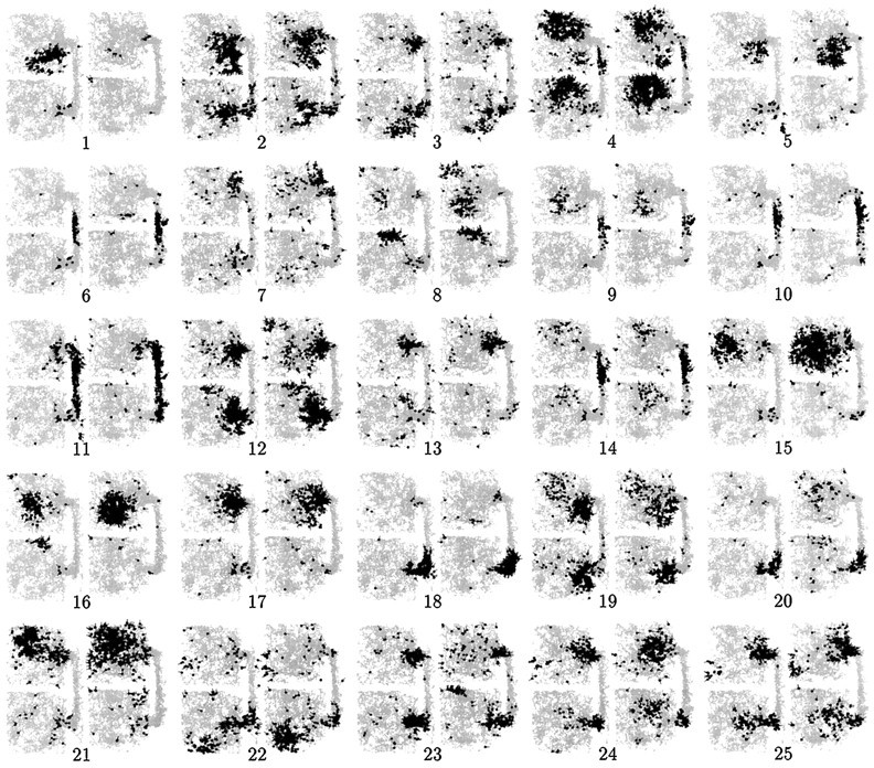
Spatial firing plots for 25 simultaneously recorded CA1 pyramidal cells from rat 1, during the first and second sessions. The two boxes were interchanged between sessions. Light gray represents the rat’s trajectory; black pointsrepresent the rat’s location at moments when the cell spiked. For this rat, the majority of cells showed distinct firing patterns in the N and S boxes, but there were a significantly above-chance number of cases of similar firing patterns (e.g., cells 2, 4, 12, 15, 19, 24, and 25). There were occasional instances of fields appearing or disappearing between sessions (e.g., cell 1), but no cases of fields switching sides when the boxes were interchanged. This implies that the different firing fields in N and S were not caused by differences in the physical features of the two boxes.

Fig. 3.

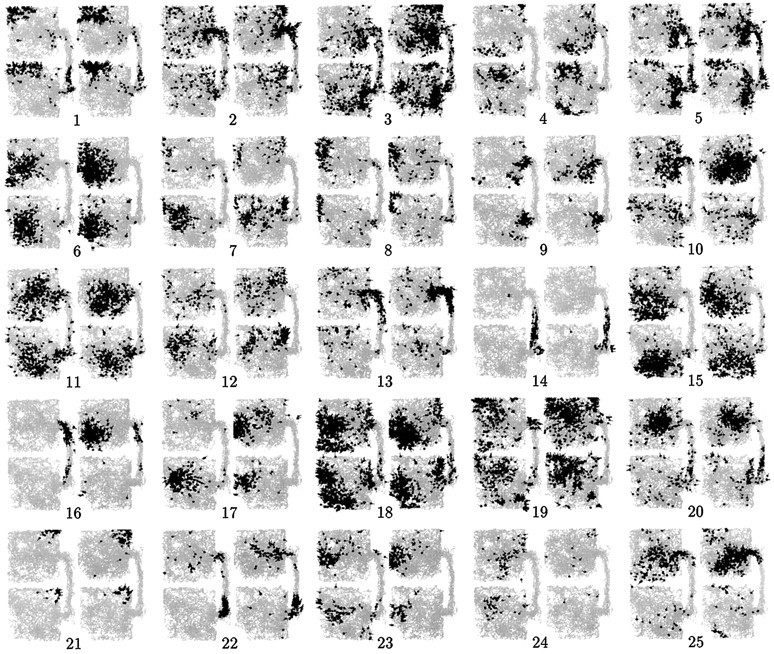
Spatial firing plots for 25 simultaneously recorded CA1 pyramidal cells from rat 2, during the first and second sessions. For this rat, the majority of cells showed similar firing patterns in the N and S boxes, but there were several instances of clearly distinct firing patterns on the two sides. In most cases these differences were maintained across sessions (e.g., cells 4, 7, 10, 20, and 25), although there were a few exceptions (e.g., cell 17). The reliable maintenance of robust differences indicates that the differences in this rat were not merely attributable to idiosyncracies of sampling. The N–S firing patterns for rats 3 and 4 resembled those for rat 2, albeit with a slightly higher level of differential N–S activity.

For each rat, at least 3 d of recording included two sessions of 12–15 min each, with the locations of boxes A and B interchanged between sessions. As illustrated by Figures 2 and 3, in no case did any field that was confined to one side during the first session switch to the corresponding location on the opposite side during the second session; that is, no cell was tied to one of the physical boxes. There were occasional instances of fields disappearing for the second session, or appearing anew, but no instances of fields moving to the opposite side. This was true for all four of the rats, although the number of meaningful examples was relatively small for rats 2, 3, and 4, because of the overall symmetry of place fields between the two sides in these rats.

Previous studies have indicated that place cell firing shows strong head direction dependence when rats travel along stereotyped trajectories, but weak or nonexistent directionality when they move in a nonstereotyped way in an open region of space (Markus et al., 1994;Muller et al., 1994). In the current experiment, the apparatus consisted of two open regions connected by a linear corridor. No attempt was made to quantify directionality, but it was generally observed that place cell activity was largely nondirectional inside the two boxes, whereas in the corridor there was a mixture of directional and non-directional fields, with numerous cells firing exclusively when the rat passed through the place field in one of the two possible directions.

The relations between N and S firing fields are described more quantitatively in Figure 4. Figure4A shows, for one late data set from each rat, the distribution of correlations between N and S firing fields. Only cells with spatial firing rates exceeding 1 Hz at some location on both sides are included (see Materials and Methods). Figure 4Aalso shows distributions generated by correlating N and S firing fields taken from different cells, reflecting the distribution that would be expected if the N and S fields were completely independent of each other. For each rat, the observed distribution differed significantly from the shuffled distribution (p < 0.005 for each; Kolmogorov–Smirnov test). Thus, even for rat 1, the number of symmetrical fields, although small, was significantly greater than chance.

Fig. 4.

Relations between firing fields in the N and S boxes. A, For each rat, the top plot shows the distribution of N–S correlations across all cells recorded during a single session on one of the later days. As a control, the distribution obtained by taking N and S firing rate maps from different, randomly chosen cells is shown below, reflecting the distribution that would be expected if the N and S firing fields of a cell were unrelated. For each rat, the observed distribution of N–S correlations differed significantly from the mixed-cell control (p < 0.005; Kolmogorov–Smirnov test). B, Distribution of N–S correlations for the first recording session of every day, from each of the four rats. Each point shows the N–S correlation of one cell, and each vertical streak shows values from one session. The horizontal coordinates are randomized slightly to make the points easier to distinguish. For rat 1, the distributions from different sessions were statistically indistinguishable. For rats 2, 3, and 4, in contrast, there was significant variability across sessions, as shown by ANOVAs (p < 0.01 for each; F test).C, Mean levels of N–S correlation for the first and last available recording sessions for each rat. For rats 1, 2, and 4, the first session came from day 1 in the apparatus; for rat 3, it came from day 5. The last session for each rat was session 1 of the day of the probe session. There was no apparent tendency for the level of N–S correlation to increase or decrease as a function of experience.

An ANOVA on the distributions shown in Figure 4Aconfirms that there were significant individual differences between rats in the level of N–S correlation (p < 0.001; F test). Not only did the rats differ from each other, but for three of them, there was significant variability across days in the level of N–S correlation. Figure 4Bshows the distribution of N–S correlations for all usable recording sessions (only the first session from any given day, however) from each rat. The distributions for rats 2, 3, and 4 varied significantly (p < 0.01 for each; F test), but the distributions for rat 1 were statistically indistinguishable across days. Despite this variability, there was no evidence for any gradual increase or decrease in the levels of N–S correlation as a function of experience in the environment. Figure 4C shows the mean level of N–S correlation for each rat on the first and last days of recording. There was not even a hint of a trend toward a difference. As described in previous reports (Hill, 1978; Wilson and McNaughton, 1993), spatially specific firing was observed from the very first entry of the rat into the environment. It was not possible to track individual cells from day to day, but in terms of population statistics there were no apparent changes as a function of experience.

To control for sensitivity to extra-maze cues, each rat on the final day of recording was given a probe session in which, contrary to the procedure on every previous session, the two boxes were reassembled for the second session in the same locations rather than interchanged, and the rat was started during the second session inside the S box. The question was whether the rat’s “expectation” that he would start in the N box would be enough to cause the N hippocampal map to be instantiated during the initial stay inside the S box. If so, this would be evidence that the differences between the N and S maps were not caused by sensitivity to extra-maze cues.

The data from the probe session were analyzed in three ways. First, firing rate maps from the S2a subsession (the first stay inside the S box during session 2) were correlated with the N and S firing rate maps from session 1. For comparison, firing rate maps from the S2b subsession (composed of all remaining visits to the S box during session 2) were also correlated with the N and S firing rate maps from session 1. Second, cells that showed clearly distinct spatial firing patterns in the N and S boxes during session 1 were examined individually to see whether their spatial firing patterns during the S2a subsession more closely resembled the N or S patterns. Third, the technique of Bayesian trajectory reconstruction was used to see whether the rat’s reconstructed position, during the initial stay in the S box, better matched his actual position or the corresponding position in the N box.

For rat 1 (with 30 pyramidal cells), the outcome of each analysis was clear and unambiguous: the N1 map was instantiated during the S2a subsession, and the session 1 maps were reinstantiated in both the N and S boxes as soon as the rat first left the S box. As shown in Figure5, the firing fields of cells during S2a correlated on average much better with their N fields during session 1 than with their S fields (p < 10⁻⁵; paired t test). For S2b, on the other hand, the correlation was better with the S fields (p < 0.005). Approximately 12 cells showed clearly distinctive spatial patterns in the N and S boxes during session 1, and without exception their firing patterns during S2a matched N better than S, whereas the opposite was true for S2b; two examples are shown in Figure 5B. As shown in Figure5C, the reconstructed trajectory fell in the N box during most of the S2a period, but reverted to match the rat’s actual location as soon as the rat passed through the corridor. During the S2a period, 87 samples of 1 sec each reconstructed to points in the N box, and only 23 reconstructed to points in the S box.

Fig. 5.

Evidence for map shifting during the probe session. A, Two examples of the behavior of individual cells from rat 1. For each cell, spatial firing plots are shown for sessions 1, 2a, and 2b. In both cases (and this was typical), the plot for session 2a resembles the N portion of the plot for session 1 much better than the S portion, whereas the plot for session 2b closely matches the plot for session 1. B, Trajectory reconstructions for the first 5 min of the probe session, for rats 1, 2, and 3. In each plot, the horizontal coordinate represents time, and the vertical coordinate represents the Y coordinate of the rat’s position, with the light gray line at the level of the wall between the two boxes. The solid line represents the rat’s actual position, and the small rectangles represent positions reconstructed from 1 sec samples of population activity, using firing rate maps from the previous session as the basis for reconstruction. For rats 1 and 3, the reconstructed locations during the initial stay in the S box fell mostly into the N box, but as soon as the rat passed through the corridor, the reconstructions reverted to mostly match the rat’s actual position. For rat 2, the reconstructions were at all times distributed almost evenly between the N and S boxes, regardless of the rat’s actual position. Trajectory reconstruction was not performed for rat 4 because of the small number of cells available.C, Correlation plots of firing rate maps derived from the S2a and S2b subsessions with maps for the same cells from the N and S boxes in session 1. Each point represents one cell. The horizontal coordinate is the correlation of the cell’s N1 firing rate map with the S2a map (top panel) or S2b map (bottom panel). The vertical coordinate is the correlation of the S1 map with the S2a map or S2b map. Thus, points lying below the diagonal indicate greater resemblance to N1 than to S1. For all four rats, the majority of points in the top plots lie below the diagonal, indicating that the population representation during S2a aligned better with N1 than with S1; however, the difference was statistically significant only for rat 1 (p < 0.00001;t test). Again for all four rats, the majority of points in the bottom plots lie above the diagonal, indicating that the population representation during S2b aligned better with S1 than with N1 (p < 0.01 for each; t test).

For the other three rats the analysis was more problematic, because the maps in the N and S boxes were so similar that it was difficult to tell which one the pattern during S2a more closely resembled. For rat 3 (30 pyramidal cells), the evidence indicates that the outcome was the same as for rat 1. First, the correlation of S2a with N1 was stronger than the correlation of S2a with S1, although the difference was not statistically significant in a t test. Second, only three cells showed clearly distinct fields between N1 and S1, but each of them showed an S2a field closely resembling the N1 field. Third, the reconstructed trajectory during the S2a period fell mostly into the N box, with 53 samples reconstructing to points in N and 30 to points in S. For this rat, as for rat 1, the firing patterns during S2b reverted to match the firing patterns during session 1.

For rat 2 (33 pyramidal cells), which had the most similar fields in N and S, none of the three analyses led to any sort of strong conclusion. The firing rate map correlations of S2a with N1 were on the whole stronger than the correlations of S2a with S1, but the difference was not statistically significant. There were four cells with distinctive fields during session 1, and their behavior in S2a was ambiguous, with one showing a firing pattern resembling its N1 field and the other three more closely resembling their S1 fields. The trajectory analysis was completely ambiguous, with 45 samples from S2a reconstructing to points in the N box, and 48 to points in the S box. For rat 4, also, no strong conclusion could be drawn, mainly because of the small number of cells in the data set (15 pyramidal cells).

In summary, then, the evidence indicates that two of the four rats showed the N1 place field maps in the S box during the first visit of session 2 and reverted back to the S1 maps as soon as they passed through the doorway and, on looking down the corridor, presumably learned that they had been started on the other side. The other two rats may have done the same thing, but the data were not strong enough to support this.

In light of recent theoretical ideas, an important question is whether the observed partial symmetry of place fields across the two boxes might be a result of confusion between what were actually orthogonal maps. If there were actually two or more orthogonal place-field maps, only one of which could be active at a time, but the visual similarity of the two sides occasionally caused the system to instantiate the “wrong” map, this would lead to the appearance of cells firing at the same location in both boxes, as was observed. The data speak against this explanation, but they do not definitively refute it.

First, the map-confusion hypothesis predicts that there should be examples of cells whose activity overlapped spatially but not temporally, that is, pairs of cells whose place fields overlapped spatially but did not fire spikes simultaneously. No examples of this type were found. Figure6A shows an illustration of the general finding: when symmetric and asymmetric cells had spatially overlapping fields, they always showed at least some degree of temporally correlated activity, on a time scale of 10 msec or less.

Fig. 6.

Data relating to the question of multiple interfering maps. A, Left, Spatial firing plots for three simultaneously recorded cells from rat 1, two having asymmetric firing fields (cells 1 and 3) and one having a symmetric field (cell 2). Right, Temporal cross-correlation plots for each pair of these three cells. Horizontal axis: seconds. Vertical axis: counts. This example illustrates the general observation that when symmetric and asymmetric fields overlapped spatially, the spike trains of the cells also overlapped temporally, indicating that the cells were unlikely to belong to separate, mutually exclusive maps.B, Trajectory reconstructions for 10 min periods from rats 1, 2, and 3. See legend of Figure 5 for explanation. In this plot, the times when the rat was inside the corridor are not shown. The reconstructions are based on populations of 38, 32, and 31 cells, respectively.

Second, the map-confusion hypothesis predicts that when the Bayesian technique is used to reconstruct the rat’s location on the basis of population activity samples, there should occasionally be periods of time when the reconstructed location lies mostly in the opposite box from the actual location, as occurred for rats 1 and 3 during the probe session, described above. As illustrated in Figure 6Bfor nonprobe sessions from three of the rats, there were of course errors in reconstruction for all of the rats, particularly rat 2 (rat 4 was not even attempted). For rat 1 these consisted for the most part of isolated samples, not concentrated in any particular part of the environment. For rats 2 and 3, there were a number of clusters of 10–20 samples in which the position repeatedly reconstructed to the “wrong” side. It is possible that these represented true failures of the system to accurately represent the rat’s location. Alternatively, it is also possible that they were merely reconstruction errors attributable to limited sampling and would go away if a larger number of cells were available. Thus, the data do not rule out the occurrence of genuine map-confusions for rats 2, 3, and 4, in which the N and S maps were very similar, but such an explanation is unlikely to hold for rat 1.

DISCUSSION

The line of thought that led to the current experiment originated from a provocative study by Quirk et al. (1992), which examined the spatial firing properties of neurons from the medial entorhinal cortex. In that study, two types of apparatus were used: first, a gray cylinder with a white cue card on the wall, and second, a similar-sized gray box with one white wall. It was found that entorhinal cells showed similar firing fields in the two environments, in contrast to an earlier study using a similar procedure (Kubie and Ranck, 1983) in which hippocampal place cells showed completely different firing patterns in the two environments. The general interpretation of these findings was that the hippocampal system transforms similar input representations into very different internal representations, a so-called “orthogonalization” process. The original aim of the current study was to gain a better understanding of this orthogonalization process, by comparing hippocampal and entorhinal representations of a pair of visually identical but spatially separated regions, the expectation being that the hippocampal representations would be orthogonal and the entorhinal ones at least partially overlapping. As it turned out, the main result of the study was to demonstrate that hippocampal “orthogonalization” is considerably less thorough and systematic than has hitherto been supposed.

The current data show that when rats moved back and forth between two environments that were similar both visually and in terms of behavioral demands, the spatial representations activated in the CA1 region of the hippocampus were neither identical nor completely distinct. Moreover, there were large variations between different individual rats, and even between different recording sessions from the same rat, in the degree of similarity. Thus the factors controlling the similarity of spatial firing patterns in the hippocampus are likely to be subtle and ephemeral. These findings raise important questions about earlier observations of nonorthogonality in entorhinal cortex (Quirk et al., 1992) and subiculum (Sharp, 1997). In neither of these studies were hippocampal recordings included as part of the same experiment; rather, comparisons were made with previous studies using similar types of apparatus. Might it not be the case that entorhinal and subicular correlations between environments are as variable as hippocampal correlations? It would clarify the issue to replicate these experiments while recording hippocampal units in exactly the same paradigm—ideally, while recording simultaneously from both areas in the same animals.

In the current study, two control manipulations were performed to test the possibility that the differences between representations were caused by physical differences between the two box areas. First, the apparatus was dismantled between recording sessions and reassembled with the two physical boxes interchanged. In every unambiguous case, place fields stayed on the same side of the apparatus and failed to follow the physical box in which they were first seen. Second, on the final day of recording, each rat was placed, during the second recording session, initially in the south box, after having been started in the north box on all previous sessions. For two of the four rats, it was clear that the north hippocampal map was instantiated during the initial period in the south box, whereas the south map was present during subsequent visits (after the rat had the chance to go through the corridor and discover which box he had actually been started in). For the other two rats, the north and south maps were too similar to make it possible to say for certain what happened. Taken together, these results make it unlikely that the firing patterns were controlled either by internal features that distinguished the two boxes from each other or by external room cues that distinguished the north region from the south region.

It is likely, then, that the differences between the north and south maps resulted from a combination of the rat’s expectations and a mechanism for remembering the rat’s movements through the corridor. The word “expectations” means, concretely, a learned association of the transfer box, or the act of being transferred, with the part of the environment in which the rat was initially placed in every session except the last. The mechanism for remembering movements could be a full-scale path integration system, as has been shown by earlier studies to exist in the rat (for review, see McNaughton et al., 1996), but a less precise sort of memory would also be sufficient to account for the present findings (e.g., “I just left the N box and turned south so the one I’m entering must be the S box”).

The data from this experiment provide compelling evidence that two distinct hippocampal maps can overlap without being identical. This is consistent with the findings of several previous studies. Markus et al. (1995) found that, when rats were required to shift from random foraging to directed running between specified points, even though no physical feature of the apparatus changed, some place cells developed new fields, but others, simultaneously recorded, kept the same fields.Tanila et al. (1997), studying small ensembles of place cells on a plus maze, found that when a rotational mismatch was created between local and distal cues, the majority of fields rotated as a consistent ensemble, but on average about 20% of fields either remapped randomly or else rotated their fields in discordance from the majority. Numerous other studies (e.g., Muller and Kubie, 1987; Shapiro et al., 1998) have described different hippocampal cells responding differently to some manipulation, but most do not impact on the issue in question, because they did not record from multiple cells simultaneously. Without simultaneous recordings, it is difficult to say whether a shift in firing is caused by all cells shifting together or by individual cells shifting differently from others.

There have been previous studies of place cells in symmetric environments, but the symmetry was rotational [for example, a gray cylinder with two diametrically opposing white cue cards (Sharp et al., 1990)] rather than translational as in the current experiment. It may well make a difference. The brain of the rat contains a “head direction” system that is intimately connected, both anatomically and functionally, with the hippocampus (Taube et al., 1990; Knierim et al., 1995; Taube, 1995). The head direction representation is dynamically stable, and only partially controlled by visual input, so it may be able to disambiguate views that are visually identical but rotated with respect to each other. With this in mind, it was considered important in the current experiment to ensure that the two boxes were identically oriented as well as visually identical, and to avoid disorienting the rats rotationally.

The observation of partially overlapping maps is a challenge to the theory that hippocampal maps are preconfigured in relation to the path-integrator mechanism and bound to exteroceptive sensory cues only as a product of learning (McNaughton et al., 1996; Samsonovich and McNaughton, 1997). If this theory were correct, and different maps were allocated for the N and S boxes, then there is no obvious reason why they would have any more in common than any other two preconfigured maps. If on the other hand the same map were allocated for both, there is no obvious reason why some cells would show different fields in N and S.

There are at least two possible ways of accounting for partial overlap. First, it may be possible to alter the original “multichart” model of Samsonovich and McNaughton (1997) into a model in which the charts are nonorthogonal and selected in a nonrandom way, such that similar-appearing environments predispose the system to allocate similar charts. One specific possibility is a “hierarchical multichart” model in which the hippocampus contains a hierarchy of maps, whose overlap depends on their relative locations in the hierarchy. A hierarchical structuring of attractors has been shown to exist in some simple neural network structures, including the Hopfield model (Amit, 1989), and can be produced in the model of Samsonovich and McNaughton (1997) by making modest changes in the structure of the model (A. Samsonovich, personal communication).

Second, the primary “cognitive map” may lie outside the hippocampus proper [perhaps in the subiculum (Sharp, 1997; Redish and Touretzky, 1997)], and hippocampal activity may be determined by a conjunction of map information and other information. Figure7 illustrates schematically how this could work. Suppose the hippocampal network H receives input from a map network M and a network C representing other information (C stands for “context”). Each hippocampal unit receives input from one map unit and one context unit, and fires only when both inputs are active. If the set of active C units is fixed and unchanging, there is a one-to-one relationship between patterns in the M layer and patterns in the H layer, so that the H units appear to form a map. A change in the set of active C units would cause a corresponding change in the set of active H units, even if the set of active M units remained identical, resulting in the appearance of a different hippocampal “map.” If only a few C units changed their activity, only a few H units would change their relationship to the M units, resulting in the appearance of partially overlapping hippocampal maps.

Fig. 7.

Schematic illustration of the concept of conjunctive coding. The idea is that each unit in the hippocampal layer H is linked to one unit in the map layer M and one unit in the context layer C. The hippocampal unit fires if and only if both inputs are active. So long as the same set of units remains active in the C layer, there is a fixed relationship between patterns in M and patterns in H. A change in the set of active C units will induce a correspondingly large change in the relationship between M patterns and H patterns. Thus, a small change in C will lead to the appearance of “partial remapping” in H.

In reality the hippocampal network is much more complicated than the simplification portrayed in Figure 7, but the general notion oforthogonalization by conjunctive coding is valid for a broad range of architectures. In a more realistic scenario, in which each hippocampal unit receives input indirectly from large groups of M units and C units, a small change in the C pattern would cause a perturbation of the observed hippocampal map, whose size depends on the parameters of the network. As the C pattern is changed more and more, at some level the hippocampal map would become completely orthogonal to what it was originally. The factors that influence this orthogonization process have been studied computationally by O’Reilly and McClelland (1994)and others (Marr, 1971; McNaughton, 1989).

Whatever the explanation is of partial remapping, the results of the current experiment demonstrate that hippocampal activity is influenced by subtle and changeable factors. Situations that are virtually identical in all sensory and behavioral respects can be associated with different hippocampal activity patterns, and it appears that the pattern present at a given time may be determined at least in part by an animal’s expectations.

REFERENCES

- 1.Amit DJ. Modelling brain function. Cambridge UP; New York: 1989. [Google Scholar]
- 2.Barnes CA, Suster MS, Shen J, McNaughton BL. Multistability of cognitive maps in the hippocampus of old rats. Nature. 1997;388:272–275. doi: 10.1038/40859. [DOI] [PubMed] [Google Scholar]
- 3.Gothard KM, Skaggs WE, McNaughton BL. Dynamics of mismatch correction in the hippocampal ensemble code for space: interaction between path integration and environmental cues. J Neurosci. 1996;16:8027–8040. doi: 10.1523/JNEUROSCI.16-24-08027.1996. [DOI] [PMC free article] [PubMed] [Google Scholar]
- 4.Hill AJ. First occurrence of hippocampal spatial firing in a new environment. Exp Neurol. 1978;62:282–297. doi: 10.1016/0014-4886(78)90058-4. [DOI] [PubMed] [Google Scholar]
- 5.Knierim JJ, Kudrimoti HS, McNaughton BL. Place cells, head direction cells, and the learning of landmark stability. J Neurosci. 1995;15:1648–1659. doi: 10.1523/JNEUROSCI.15-03-01648.1995. [DOI] [PMC free article] [PubMed] [Google Scholar]
- 6.Kubie JL, Ranck JB., Jr . Sensory-behavioral correlates of individual hippocampal neurons in three situations: space and context. In: Seifert W, editor. Neurobiology of the hippocampus. Academic; New York: 1983. pp. 433–447. [Google Scholar]
- 7.Markus EJ, Barnes CA, McNaughton BL, Gladden VL, Skaggs WE. Spatial information content and reliability of hippocampal CA1 neurons: effects of visual input. Hippocampus. 1994;4:410–421. doi: 10.1002/hipo.450040404. [DOI] [PubMed] [Google Scholar]
- 8.Markus EJ, Qin YL, Leonard B, Skaggs WE, McNaughton BL, Barnes CA. Interactions between location and task affect the spatial and directional firing of hippocampal neurons. J Neurosci. 1995;15:7079–7094. doi: 10.1523/JNEUROSCI.15-11-07079.1995. [DOI] [PMC free article] [PubMed] [Google Scholar]
- 9.Marr D. Simple memory: a theory for archicortex. Philos Trans R Soc Lond B Biol Sci. 1971;262:23–81. doi: 10.1098/rstb.1971.0078. [DOI] [PubMed] [Google Scholar]
- 10.McNaughton BL. Neuronal mechanisms for spatial computation and information storage. In: Nadel L, Cooper LA, Culicover P, Harnish RM, editors. Neural connections, mental computations. MIT; Cambridge, MA: 1989. pp. 285–350. [Google Scholar]
- 11.McNaughton BL, O’Keefe J, Barnes CA. The stereotrode: a new technique for simultaneous isolation of several single units in the central nervous system from multiple unit records. J Neurosci Methods. 1983;8:391–397. doi: 10.1016/0165-0270(83)90097-3. [DOI] [PubMed] [Google Scholar]
- 12.McNaughton BL, Chen LL, Markus EJ. “Dead reckoning,” landmark learning, and the sense of direction: a neurophysiological and computational hypothesis. J Cognit Neurosci. 1991;3:190–202. doi: 10.1162/jocn.1991.3.2.190. [DOI] [PubMed] [Google Scholar]
- 13.McNaughton BL, Barnes CA, Gerrard JL, Gothard K, Jung MW, Knierim JJ, Kudrimoti H, Qin Y, Skaggs WE, Suster M, Weaver KL. Deciphering the hippocampal polyglot: the hippocampus as a path integration system. J Exp Biol. 1996;199:173–185. doi: 10.1242/jeb.199.1.173. [DOI] [PubMed] [Google Scholar]
- 14.Muller RU, Kubie JL. The effects of changes in the environment on the spatial firing of the hippocampal complex-spike cells. J Neurosci. 1987;7:1951–1968. doi: 10.1523/JNEUROSCI.07-07-01951.1987. [DOI] [PMC free article] [PubMed] [Google Scholar]
- 15.Muller RU, Bostock E, Taube JS, Kubie JL. On the directional firing properties of hippocampal place cells. J Neurosci. 1994;14:7235–7251. doi: 10.1523/JNEUROSCI.14-12-07235.1994. [DOI] [PMC free article] [PubMed] [Google Scholar]
- 16.O’Keefe J, Nadel L. The hippocampus as a cognitive map. Clarendon; Oxford: 1978. [Google Scholar]
- 17.O’Keefe J, Recce ML. Phase relationship between hippocampal place units and the EEG theta rhythm. Hippocampus. 1993;3:317–330. doi: 10.1002/hipo.450030307. [DOI] [PubMed] [Google Scholar]
- 18.O’Reilly RC, McClelland JL. Hippocampal conjunctive encoding, storage, and recall: avoiding a trade-off. Hippocampus. 1994;4:661–682. doi: 10.1002/hipo.450040605. [DOI] [PubMed] [Google Scholar]
- 19.Press WH, Teukolsky SA, Vetterling WT, Flannery BP. Numerical recipes in C. Cambridge UP; Cambridge: 1992. [Google Scholar]
- 20.Quirk GJ, Muller RU, Kubie JL, Ranck JB., Jr The positional firing properties of medial entorhinal neurons: description and comparison with hippocampal place cells. J Neurosci. 1992;12:1945–1963. doi: 10.1523/JNEUROSCI.12-05-01945.1992. [DOI] [PMC free article] [PubMed] [Google Scholar]
- 21.Redish AD, Touretzky DS. Cognitive maps beyond the hippocampus. Hippocampus. 1997;7:15–35. doi: 10.1002/(SICI)1098-1063(1997)7:1<15::AID-HIPO3>3.0.CO;2-6. [DOI] [PubMed] [Google Scholar]
- 22.Samsonovich A, McNaughton BL. Path integration and cognitive mapping in a continuous attractor neural network model. J Neurosci. 1997;17:5900–5920. doi: 10.1523/JNEUROSCI.17-15-05900.1997. [DOI] [PMC free article] [PubMed] [Google Scholar]
- 23.Shapiro ML, Tanila H, Eichenbaum H. Cues that hippocampal place cells encode: dynamic and hierarchical representation of local and distal stimuli. Hippocampus. 1997;7:624–642. doi: 10.1002/(SICI)1098-1063(1997)7:6<624::AID-HIPO5>3.0.CO;2-E. [DOI] [PubMed] [Google Scholar]
- 24.Sharp PE. Subicular cells generate similar spatial firing patterns in two geometrically and visually distinct environments: comparison with hippocampal place cells. Behav Brain Res. 1997;85:71–92. doi: 10.1016/s0166-4328(96)00165-9. [DOI] [PubMed] [Google Scholar]
- 25.Sharp PE, Kubie JL, Muller RU. Firing properties of hippocampal neurons in a visually symmetrical environment: contributions of multiple sensory cues and mnemonic processes. J Neurosci. 1990;10:3093–3105. doi: 10.1523/JNEUROSCI.10-09-03093.1990. [DOI] [PMC free article] [PubMed] [Google Scholar]
- 26.Skaggs WE, McNaughton BL, Wilson MA, Barnes CA. Theta phase precession in hippocampal neuronal populations and the compression of temporal sequences. Hippocampus. 1996;6:149–172. doi: 10.1002/(SICI)1098-1063(1996)6:2<149::AID-HIPO6>3.0.CO;2-K. [DOI] [PubMed] [Google Scholar]
- 27.Tanila H, Shapiro ML, Eichenbaum H. Discordance of spatial representation in ensembles of hippocampal place cells. Hippocampus. 1997;7:613–623. doi: 10.1002/(SICI)1098-1063(1997)7:6<613::AID-HIPO4>3.0.CO;2-F. [DOI] [PubMed] [Google Scholar]
- 28.Taube J. Head direction cells recorded in the anterior thalamic nuclei of freely moving rats. J Neurosci. 1995;15:70–86. doi: 10.1523/JNEUROSCI.15-01-00070.1995. [DOI] [PMC free article] [PubMed] [Google Scholar]
- 29.Taube JS, Muller RU, Ranck JB., Jr Head direction cells recorded from the post-subiculum in freely moving rats. I. Description and quantitative analysis. J Neurosci. 1990;10:420–435. doi: 10.1523/JNEUROSCI.10-02-00420.1990. [DOI] [PMC free article] [PubMed] [Google Scholar]
- 30.Thompson LT, Best PJ. Place cells and silent cells in the hippocampus of freely behaving rats. J Neurosci. 1989;9:2382–2390. doi: 10.1523/JNEUROSCI.09-07-02382.1989. [DOI] [PMC free article] [PubMed] [Google Scholar]
- 31.Wiener SI. Spatial, behavioral and sensory correlates of hippocampal CA1 complex spike cell activity: implications for information processing. Prog Neurobiol. 1996;49:335–361. doi: 10.1016/0301-0082(96)00019-6. [DOI] [PubMed] [Google Scholar]
- 32.Wilson MA, McNaughton BL. Dynamics of the hippocampal ensemble code for space. Science. 1993;261:1055–1058. doi: 10.1126/science.8351520. [DOI] [PubMed] [Google Scholar]
- 33.Zhang K, Ginsburg I, McNaughton BL, Sejnowski TJ. Interpreting neuronal population activity by reconstruction: a unified framework with application to hippocampal place cells. J Neurophysiol. 1998;79:1017–1044. doi: 10.1152/jn.1998.79.2.1017. [DOI] [PubMed] [Google Scholar]
- 34.Zipser D. A computational model of hippocampal place fields. Behav Neurosci. 1985;99:1006–1018. doi: 10.1037//0735-7044.99.5.1006. [DOI] [PubMed] [Google Scholar]