Feature Extraction by Burst-Like Spike Patterns in Multiple Sensory Maps

Abstract

In most sensory systems, higher order central neurons extract those stimulus features from the sensory periphery that are behaviorally relevant (e.g., Marr, 1982; Heiligenberg, 1991). Recent studies have quantified the time-varying information carried by spike trains of sensory neurons in various systems using stimulus estimation methods (Bialek et al., 1991; Wessel et al., 1996). Here, we address the question of how this information is transferred from the sensory neuron level to higher order neurons across multiple sensory maps by using the electrosensory system in weakly electric fish as a model. To determine how electric field amplitude modulations are temporally encoded and processed at two subsequent stages of the amplitude coding pathway, we recorded the responses of P-type afferents and E- and I-type pyramidal cells in the electrosensory lateral line lobe (ELL) to random distortions of a mimic of the fish’s own electric field. Cells in two of the three somatotopically organized ELL maps were studied (centromedial and lateral) (Maler, 1979; Carr and Maler, 1986). Linear and second order nonlinear stimulus estimation methods indicated that in contrast to P-receptor afferents, pyramidal cells did not reliably encode time-varying information about any function of the stimulus obtained by linear filtering and half-wave rectification. Two pattern classifiers were applied to discriminate stimulus waveforms preceding the occurrence or nonoccurrence of pyramidal cell spikes in response to the stimulus. These signal-detection methods revealed that pyramidal cells reliably encoded the presence of upstrokes and downstrokes in random amplitude modulations by short bursts of spikes. Furthermore, among the different cell types in the ELL, I-type pyramidal cells in the centromedial map performed a better pattern-recognition task than those in the lateral map and than E-type pyramidal cells in either map.

Any comprehensive characterization of sensory information processing by neuronal networks has to rely on a wide range of experimental and theoretical approaches (Reichardt and Poggio, 1976; Marr, 1982; Koch, 1998). Knowledge of the anatomy of sensory pathways and of the microstructure of neuronal circuits as well as of electrophysiological response properties of single neurons and their involvement in behavior are required (Heiligenberg, 1991). In addition, a quantitative understanding of the encoding and processing of sensory information in single and multiple neuronal spike trains is also needed. Information theoretical approaches and methods drawn from statistical signal processing have long been applied to examine the latter aspects (Marmarelis and Naka, 1972; Marmarelis and McCann, 1973). However, in many cases, the functional and behavioral significance of such studies remained unclear. Because the electrosensory system is relatively simply structured and the role of its circuitry in processing behaviorally relevant signals across multiple parallel sensory pathways is well known, it represents an ideal model to investigate, in a quantitative manner, the computational mechanisms underlying the encoding and processing of sensory information at the single neuron and network level (Konishi, 1991).

Weakly electric fish generate electric fields for the active detection of objects and for communication (for review, see Heiligenberg, 1991;Bastian, 1994; Metzner and Viete, 1996a,b). In Eigenmannia, electric signals that follow an almost sinusoidal time course are produced by continuous discharges of an electric organ at a rate between 150 and 600 Hz. Two types of electroreceptors exist to monitor electric fields: low-frequency ampullary and high-frequency tuberous (Zakon, 1986; Heiligenberg, 1993). Tuberous electroreceptors and their associated primary afferents are tuned to the dominant spectral frequency range of the animal’s own electric organ discharge (EOD) and consist of two subclasses. T-type afferents fire phase-locked to the zero-crossings of the EOD waveform. P-type afferents, on the other hand, fire intermittently, with highly fluctuating response latencies, and they encode changes in the electric field amplitude (Scheich et al., 1973; Bastian and Heiligenberg, 1980; Bastian, 1981a, 1986b;Wessel et al., 1996).

All electroreceptor afferents terminate in the electrosensory lateral line lobe (ELL) of the hindbrain in a somatotopic manner. The ELL consists of four mediolaterally adjacent segments or “maps” (Fig.1). The medial segment receives input from ampullary afferents, whereas the three remaining segments (centromedial, centrolateral, and lateral) are each innervated by one collateral of tuberous afferents (Heiligenberg and Dye, 1982; Carr and Maler, 1986). Tuberous afferents excite basilar pyramidal cells directly and inhibit nonbasilar pyramidal cells indirectly via granule cells. Thus, an increased firing rate in a P-type afferent, reflecting a rise in stimulus amplitude, will excite a basilar (E-type) pyramidal cell and inhibit a nonbasilar (I-type) pyramidal cell (Bastian and Heiligenberg, 1980; Saunders and Bastian, 1984).

Fig. 1.

A, Frontal section through the hindbrain (right half) of Eigenmannia showing the four segments, or maps, of the electrosensory lateral line lobe (ELL). MS, Medial (ampullary) segment; three tuberous segments: CMS, centromedial, CLS, centrolateral, LS, lateral;Cer, cerebellum, VIII, octavolateral nerve (containing the electrosensory afferents); layers of the tuberous ELL segments: dnl, deep neuropil layer (contains collaterals of electrosensory afferents), sl, spherical cell layer (contains phase coding cells; serves as landmark), gl, granule cell layer (contains inhibitory interneurons), pl, pyramidal cell layer (contains E- and I-units shown in B),ml, molecular layer (contains apical dendrites of pyramidal cells). B, Camera lucida drawings of an E-type (top) and I-type (bottom) pyramidal cells that were labeled intracellularly with neurobiotin.

Several computational mechanisms for the transfer of electric field amplitude information were suggested from the mean response characteristics of pyramidal cells. For instance, pyramidal cells may combine half-wave rectification with transmission of time-varying information on temporal changes in the stimulus waveform (such as the first derivative of the electric field amplitude modulation) (Enger and Szabo, 1965; Bastian 1986b). Alternatively, they might convey time-varying information on specific frequency ranges contained in the amplitude modulations of the stimulus (Maler, 1989; Rose and Call, 1992, 1993; Fortune and Rose, 1997). The aim of the present study was to test these hypotheses and determine how amplitude modulations are temporally encoded and processed between the first two stages in the segregated pathways (Metzner and Juranek, 1997) of the electrosensory system.

A short report of parts of our results has been published previously (Gabbiani et al., 1996).

MATERIALS AND METHODS

Preparation. Thirty-five adult specimens ofEigenmannia species from 12 to 20 cm body length were used in this study. The fish had either been bred and raised in the laboratory or were purchased from a tropical fish wholesaler (Bailey’s, San Diego, CA). They were immobilized by intramuscular injection of Flaxedil (<5 μg/gm body weight) (gallamine triethiodide; Sigma, St. Louis, MO), gently suspended in the center of the experimental aquarium (water conductivity, 90–110 μS/cm, pH 7; temperature, 26–28°C) by a foam-lined forceps with only the dorsal surface of their head protruding above the water surface, and respirated with a stream of aquarium water via a silicone-coated glass tube inserted in their mouth. A small plexiglass rod was glued to the parietal bone under local anesthesia (2% lidocaine; Western Medical Supplies, Arcadia, CA) to further stabilize the fish. The experimental tank was situated on a vibration isolation table (Newport, Fountain Valley, CA). Although Flaxedil strongly attenuated the fish’s EOD, residual signals (amplitude, 50 μV to 1 mV) locked to the spinal command neurons could still be monitored with a suction electrode fitted over the tip of the tail. Curarization reduced the EOD amplitude below the threshold level of electroreceptors. The electrosensory system was stimulated using an EOD mimic consisting of a sinusoidal stimulus (S1) that was applied between an electrode in the mouth and an electrode near the tip of the tail and is described in more detail below.

Electrophysiology. For recordings of receptor afferents, the posterior branch of the anterior lateral line nerve just rostral to the operculum was exposed. This allowed us to record extracellularly the activity of single P-type electroreceptor afferents. For intracellular recordings from pyramidal cells, the ELL was reached by removing part of the occipital bone overlying the caudal cerebellum (∼3 mm²) under local anesthesia (lidocaine). Intracellular signals were recorded with glass micropipettes filled with 3 m KCl (resistance, 40–60 MΩ for extracellular and 70–130 MΩ for intracellular recordings; borosilicate glass was pulled on a Sutter P-87 (Flaming-Brown, Novato, CA). Penetrations were obtained by applying brief overcompensation of capacitance neutralization or slight mechanical tapping of the headstage and of the microdrive or both. Cell membrane potentials were sometimes stabilized during data acquisition by passage of a weak, hyperpolarizing current (corresponding to a hyperpolarization of the membrane potential of ∼5 mV). Recording signals were amplified with an intracellular electrometer (World Precision Instruments, WPI 767, Sarasota, FL) and stored on a video tape using a PCM recording adapter (sample rate, 40 kHz; Vetter 3000A, Rebersburg, PA). They were subsequently converted from analog to digital using a commercial data analysis system (sample rate, 2 or 4 kHz/channel; Datawave, Denver, CO).

Anatomy. The ELL is highly laminated (Fig. 1), and the somata of large pyramidal cells are situated in a central layer that extends dorsoventrally over a distance of 200 μm. GABAergic polymorphic cells and few small pyramidal cells are found in the ventral region of this pyramidal cell layer and appear to make only intrinsic connections within the ELL (Bastian et al., 1993; Maler and Mugnaini, 1994). We recorded only from the large pyramidal cells of the centromedial (CMS) and lateral (LS) segments that are situated in the central pyramidal cell layer and project to higher order structures. This layer can be identified easily by anatomical and physiological criteria. For instance, the center of the pyramidal cell layer is located ∼200 μm dorsal to the spherical cell layer, which is only ∼100 μm thick and physiologically very distinct. Spherical cells are innervated by T-receptor afferents and fire, in contrast to pyramidal cells, strictly phase-locked to the EOD mimic even at the low stimulus amplitudes used in this study. This very reliable landmark allowed us to limit data collection to the pyramidal cell layer and in some cases to the molecular layer that contains the large apical dendritic trees of pyramidal cells (Carr and Maler, 1986). Pyramidal cell activity was recorded with electrodes filled with neurobiotin (2% in 3 m KCl) (Vector Laboratories, Eugene, OR) for intracellular labeling (Metzner and Heiligenberg, 1991; Heiligenberg et al., 1996). In all cases, the subsequent histological analysis revealed label in pyramidal cells only (Fig. 1). If no intracellular labeling could be performed, the recording site was histologically verified by setting electrolytic lesions at the conclusion of the experiment using a high-frequency current (Hyfrecator 733; Bircher Medical Systems, Irvine, CA) (bipolar setting at 15 W for 10 sec) (Metzner, 1993). The current was applied through a low-impedance recording electrode (<20 MΩ) positioned at the most lateral (in the case of the centromedial ELL segment) and most medial recordings (in the case of the lateral ELL segment) at the depth of the pyramidal cell layer. The fish was euthanized with MS-222 (tricaine-methane sulfonate; Sigma) and perfused with 4% paraformaldehyde in 0.1 m phosphate buffer. Brains were post-fixed overnight and then cut on a vibratome in sections of 50 μm thickness. Sections were mounted, dehydrated, counterstained with neutral red or cresyl violet (Nissl stain), and coverslipped. The nomenclature of brain structures used for the light-microscopic analysis follows Maler et al. (1991).

Stimulation protocols. The stimulus presentation followed the convention described in Wessel et al. (1996). Briefly, the voltage V(t) of the electric field mimic had a mean amplitudeA₀ and a carrier frequencyf_carrier and was modulated randomly (random amplitude modulations, RAMs) according to V(t) = A₀ [1 + s(t)] cos (2πf_carriert). The carrier frequency was set at the fish’s electric organ frequency before immobilization and was above 350 Hz in all fish used for our experiments. The mean amplitude A₀ took values between 1 and 5 mV/cm near and perpendicular to the head of the fish. The stimulus s(t) had a flat power spectrum up to a cut-off frequency,f_c, which in the present study was varied between 2 and 40 Hz. This white noise was generated by playing a blank tape on a tape recorder [bandwidth, DC to 10 kHz, signal-to-noise ratio (SNR) = 50 dB; Racal Instruments, UK], which was subsequently filtered by a flat-amplitude, low-pass filter (two four-pole Butterworth filters in series; Wavetek Rockland 452, San Diego, CA). The SD, ς, of the stimulus was varied between 0.1 and 0.45 V, corresponding to variations between 10 and 45% of the mean electric field amplitude. This range of values was slightly higher than the one used in Wessel et al. (1996) and led to more reliable responses in pyramidal cells. For the lower range of cut-off frequencies,f_c, used in this study as compared withWessel et al. (1996), A(t) = A₀[1 + s(t) ] remained positive up to ς = 0.45 V, i.e., no phase changes were introduced in the voltageV(t) relative to the carrier signal cos(2πf_carriert).

At the beginning of each recording, the response of the cell to sinusoidal amplitude modulations between 2 and 10 Hz of a stimulus with a carrier frequency similar to the animal’s own EOD frequency was determined. This allowed us to easily classify the cell as E- or I-unit (Metzner and Heiligenberg, 1991). Subsequently, the response of the cell to RAMs was tested. Each stimulus configuration was presented for 2.5 min. Various stimulus configurations were tested by changing the parameters f_c,A₀, and ς pseudorandomly between stimulus presentations, as time permitted. At least three configurations were required to include a cell recording into our data base. The maximum time we recorded intracellularly from a pyramidal cell was 101 min.

Spike train analysis. To study the spontaneous activity of pyramidal cells, the spike peak occurrence times were selected and resampled at 2 kHz. Interspike interval (ISI) distributions, including means and coefficients of variation (CVs), autocorrelation functions, power spectra, and variance versus mean spike count curves were computed using standard methods, as described in Gabbiani and Koch (1998). The analysis of stimulus-driven activity was also performed on spike occurrence times and stimuli initially digitized at 2 kHz. For very low stimulus cut-off frequencies (≤5 Hz), the sampling rate was divided by a factor of 4, and the recording time was multiplied by the same factor, to improve temporal averaging at the expense of spectral frequency resolution.

Linear stimulus estimation. Linear estimation of the stimulus from the spike trains of pyramidal cells and P-receptor afferents was performed and quantified as described in detail in Wessel et al. (1996) and Gabbiani and Koch (1998, Sec 9.7). Briefly, the autocorrelation function of the spike train and the cross-correlation with the stimulus were computed and used to obtain a Wiener–Kolmogorov filter that was then convolved with the spike train, yielding an optimal linear estimate of the stimulus in the mean square sense (Gabbiani and Koch, 1998). The accuracy of this stimulus estimation method and of the one described in the following paragraph were assessed by computing the root mean square error, ε, between the estimate and the stimulus. The coding fraction was then defined from the root mean square error, ε, and the SD, ς, of the stimulus as γ = 1 − ε/ς. The coding fraction takes the maximum value of 1 when the stimulus is perfectly estimated (ε = 0) and the minimum value of 0 when estimation is at chance level (ε = ς) (Gabbiani and Koch, 1996). Thus, the coding fraction γ provides an objective estimate of the time-varying information encoded in a neuronal spike train, as assessed by an ideal observer. The accuracy of stimulus estimations was further characterized in the frequency domain by computing signal-to-noise ratios (SNRs) as a function of stimulus frequency (see Fig. 6). A value of 1 for SNR(f) at a given frequency, f, means that estimation of this particular frequency is at chance level, whereas perfect estimation corresponds to an infinite SNR (Gabbiani and Koch, 1996). In addition to the stimulus itself, three linear and non-linear functions of the stimulus were estimated by the same method. These included, after subtraction of the mean stimulus, first, positively and negatively half-wave rectified stimuli; second, the temporal derivative of the stimulus; and third, positively and negatively half-wave rectified temporal derivatives. Temporal derivatives were computed by linear convolution of the stimuli with a digital differentiation filter. To suppress the amplification of high-frequency noise inherent to such a numerical computation, the differentiation filter was convolved with a carefully selected Kaiser window, as explained in Hamming (1989, Sec 9.7) and Oppenheim and Schaffer (1989).

Fig. 6.

Spontaneous activity of an E-type pyramidal cell in CMS (no external stimulus present). A, ISI distribution, with a mean interspike interval of 60 msec and a CV equal to 1.56. Thearrow indicates the maximal interspike interval (t_max = 19 msec) between two spikes assigned to the same burst event. The range of values for the mean and CV observed in 36 cells is given in the inset. B, The autocorrelation function of the spike train (thick line) showed a peak at the preferred intraburst interspike interval (15 msec). This peak disappears in the autocorrelation function of the events (thin line), which consist of the original isolated spikes and one spike for each burst in the spike train (Bair et al., 1994). The δ function singularity of both autocorrelation functions at t = 0 has been subtracted. C, The probability distribution of the number of spikes per event was always well fitted by a straight line in logarithmic coordinates (Pearson correlation coefficient r = −0.998; observed range, from −0.957 to −0.999). The arrow indicates a single burst event containing 16 spikes that was not included in the fit and was classified as an outlier (total number of events, 1012). D, Plot of the slope, a, versus the intercept parameter,b, describing the statistics of spikes per event (dashed line, best linear fit). Different symbolsindicate responses obtained from different pyramidal cell types and ELL maps (n = 32 pyramidal cells).E_CMS, E-units in centromedial map; E_LS, E-units in lateral map; I_CMS, I-units in centromedial map; I_LS, I-units in lateral map.

Nonlinear stimulus estimation. The (half-wave-rectified) stimulus and its (half-wave-rectified) temporal derivative were also estimated from the spike trains of pyramidal cells by a quadratic algorithm, which took possible nonlinear interactions in the encoding of detailed time-course information into account that could have taken place between two spike occurrence times. The implementation used a straightforward modification of the fast orthogonal method described inKorenberg (1988). Because of the computational burden of such general quadratic algorithms (Koh and Powers, 1985), the stimuli and spike trains were first resampled with a resolution of 20 msec, corresponding to a sample rate of 50 Hz. This sampling rate was sufficient to resolve the time-course of stimuli with a cut-off frequency below 25 Hz (see Fig. 6B, C). During the resampling of pyramidal cell spike trains, two spikes occurring in the same 20 msec bin were replaced by a single event of doubled amplitude {i.e., δ(t − t₁) + δ(t − t₂) → 2 δ(t − t₃) for t₁,t₂ in [t₃ − 10 msec;t₃ + 10 msec], where δ(t − t_i) represents the occurrence of a spike att_i, i = 1, 2, 3}. The down-sampling allowed us to use linear and quadratic filters of manageable size (31 and 31 × 31 elements, respectively) to cover the time windows of interest (±300 msec around each spike). Linear estimation of the stimulus from resampled pyramidal spike trains were first compared with those obtained at a sampling rate of 2 kHz. The estimation filters and the fraction of the stimulus encoded that were obtained with these two methods were identical, indicating that temporal modulations in the instantaneous firing rate of pyramidal cells below 20 msec did not carry substantial information about the stimulus time-course. In contrast, stimulus estimations from 50 Hz down-sampled P-receptor afferent spike trains were substantially worse than those obtained at a 2 kHz sampling rate, indicating that modulations in the instantaneous firing rate of P-receptor afferents at time scales shorter than 20 msec carried substantial information. Therefore, quadratic estimation methods were not pursued further with P-receptor afferent spike trains.

Feature extraction. We assessed the ability of pyramidal cell and P-receptor spikes to convey information about the presence of temporal features, such as up- and downstrokes in random modulations of the electric field amplitude, by discriminating stimulus waveforms preceding the occurrence or nonoccurrence of spikes in response to the stimulus by using two pattern classifiers (Fisher and Euclidian, respectively). In the following, we will first explain how the stimulus waveforms were obtained and then describe how the two classifiers were defined and how the classification error characterizing their performance was computed.

Each spike train and the corresponding stimulus s(t) were binned using three bin sizes between Δt = 0.5 msec (corresponding to the sampling rate of 2 kHz for the spike occurrence times) and a maximal bin size Δt_max. The maximal bin size was determined from the requirement that no more than one spike should fall in a given bin. In general, this requirement was slightly alleviated by the fact that in <1.8% of all spike occurrences, two spikes were allowed to fall in the same bin. This accounted for the rare occurrence of exceptionally close spikes and for an unfavorable placement of the bins with respect to the spike train. For spikes of pyramidal cells, Δt ranged between 3 and 15 msec, whereas for P-receptor afferents Δt ranged from 0.5 to 4.5 msec because of their higher firing rates (see Fig. 7A). The wave-form of the RAM that preceded the bin [t − Δt;t] was defined as the 101 dimensional stimulus vector s_t = (s(t − 100 Δt), …, s(t) ), and the variable λ_t took the value 1 or 0 depending on whether a spike occurred in the bin [t− Δt;t]. Let P (s‖λ = 1) and P(s‖λ = 0) be the two distributions of stimulus vectors conditioned on the occurrence or nonoccurrence of a spike in a bin of size Δt. The collection of stimulus vectors belonging to these distributions was determined from the experimental data by considering successively each time point t = n Δt for n ranging from 101 to the largest integer smaller than T /Δt, with T being the duration over which one particular stimulus configuration was presented (see above; usually, T = 140 sec). Each vectors_t was assigned to P(s‖λ = 1) or to P(s‖λ = 0) according to whether (λ_t = 1) or not (λ_t = 0) a spike occurred in the bin [t − Δt;t] (Fig.2).

Fig. 7.

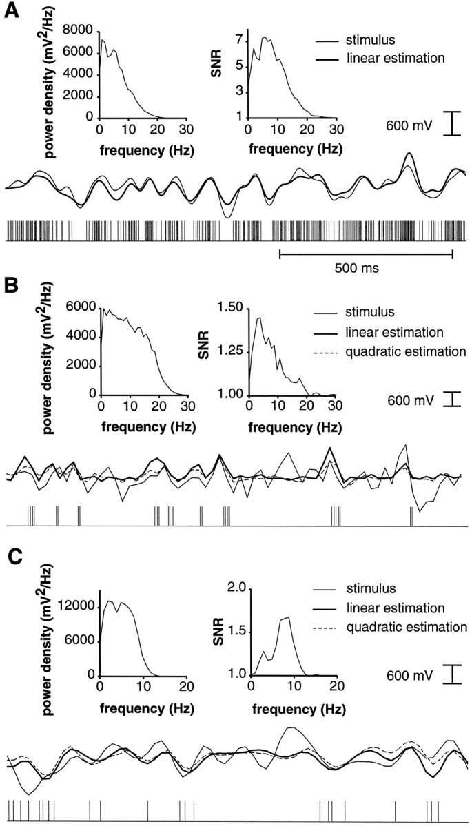
Examples of linear and quadratic stimulus estimations for responses of P-receptor afferents (A), E-type (B), and I-type pyramidal cells (C). For all three examples (A–C), spike trains are symbolized in each bottom row, the corresponding RAMs (= stimuli) are indicated in the center and superimposed with their linear, and inB and C only, quadratic estimates obtained from the spike trains. Each top row contains two graphs showing the power spectral density of the stimulus as a function of stimulus frequency (left graphs) and SNR in the frequency domain for linear estimation (right graphs). A, P-receptor afferents encoded the detailed time-course of the stimulus by modulating their instantaneous firing frequency. Note the much higher sustained firing rate than that observed in pyramidal cells (seeB and C) (mean firing rate: 221 Hz; coding fraction γ = 0.76; stimulus parameters: A₀ = 1.2 mV, ς = 0.26 V, f_c = 9 Hz).B, Linear and quadratic estimation for an E-type pyramidal cell from CMS (E_cms; mean firing rate: 17 Hz; γ_lin = 0.09; γ_quadr = 0.13; stimulus parameters: A₀ = 3.0 mV, ς = 0.32 V,f_c = 18 Hz). The stimulus was resampled at a 50 Hz sampling rate to compute the quadratic estimate (see Materials and Methods). The stimulus as well as the linear and quadratic estimates are therefore illustrated at this sampling rate. C, Same as in B for an I-type pyramidal cell from CMS (I_cms; mean firing rate: 13 Hz; γ_lin = 0.11; γ_quadr = 0.15; stimulus parameters: A₀ = 5.0 mV, ς = 0.34 V,f_c = 9 Hz).

Fig. 2.

Schematization of the data analysis performed for the feature extraction method. Center panel, Each stimulus and spike train was subdivided into short bins (labeleda–r) containing at most one spike. The collection of stimuli preceding each bin was separated into two distributions, P(s‖λ = 1) and P(s‖λ = 0), according to whether a spike occurred in the corresponding bin (c, d, g, j, k, m, q, r) or not (a, b, e, f, h, i, l, n–p). In the example depicted here, spikes occur preferentially after a RAM upstroke (as for E-type pyramidal cells). The separation of the two distributions and, thus, the ability of spikes to reliably convey the presence of an upstroke was then assessed using a linear classifier. Side boxes, Means m₀ (left, top graph) andm₁ (right, top graph) of the stimulus preceding no spike occurrence (left box) and the occurrence of a spike (right box) for an E-unit in the CMS as well as the covariance matrices, Σ₀ (left, bottom graph) and Σ₁ (right, bottom graph) characterizing the second order variations of P(s‖λ = 0) and P(s‖λ = 1) aroundm₀ and m₁ (stimulus parameters: A₀ = 3.0 mV/cm, f_c = 44 Hz, ς = 0.32 V; bin size Δt = 3.5 msec). Note the difference in scale between the two top panels. Because our stimuli are stationary and zero mean, the means m₀ andm₁ are related according to p₀m₀ + p₁m₁ = 0 (with p₁ = probability of a spike in bin Δt , and p₀ = probability of no spike occurrence in bin Δt ).

The separation of the distributions P(s‖λ = 0) and P(s‖λ = 1) in stimulus space was assessed by the ability of a statistical pattern classifier to discriminate among them. Consider a linear classifier of the form:

$$h_{\mathbf{\text{f}},\theta }(\mathbf{\text{s}})={\mathbf{\text{f}}}^T·\mathbf{\text{s}}-\theta ,$$ Equation 1

where the dot denotes matrix multiplication and the notationx^T for a vector x denotes the transposed vector, obtained by exchanging the rows and columns ofx. According to Equation 1, for a fixed feature vectorf and threshold θ, a stimulus s is classified as belonging to class 1 (i.e., the class of stimuli eliciting a spike) or class 0 (i.e., the class of stimuli eliciting no spike) by projecting s onto f and comparing the value of the projection to the threshold θ. Iff^T·s is larger than threshold [corresponding to h_f,θ(s) > 0], then sis assigned to class 1; otherwise s is assigned to class 0.

Fisher classifier. The performance of the classifier of Equation 1 relies on an appropriate choice of the feature vectorf and the threshold θ. The optimal feature vectorf was determined by maximizing Fisher’s linear discriminant function. Let m₀ and m₁be the mean values of the conditional distributions P(s‖λ = 0) and P(s‖λ = 1), respectively, and denote by Σ₀ and Σ₁ the corresponding covariances:

$${\mathrm{\Sigma }}_i=\langle (\text{s}-{\mathbf{\text{m}}}_i)·(\text{s}-{\mathbf{\text{m}}}_i{)}^T{\rangle }_i,$$ Equation 2

where the average 〈·〉_i is over the distribution P(s‖λ = i),i = 0, 1 (Figs. 2, 4A–D). The covariance matrices defined in Equation 2 characterize to a first approximation the variances and the correlations among the components of the stimulus vector s for the two classesi = 0, 1. Estimates ofm₀, m₁, Σ₀, and Σ₁ were obtained using maximum likelihood estimators. The feature vector f used to separate the distributions P(s‖λ =i), i = 0, 1 was obtained by maximizing the signal-to-noise ratio:

$$SNR(\mathbf{\text{f}})=\frac{[{\mathbf{\text{f}}}^T·({\mathbf{\text{m}}}_1-{\mathbf{\text{m}}}_0){]}^2}{{\mathbf{\text{f}}}^T·\left(\frac{1}{2}{\mathrm{\Sigma }}_0+\frac{1}{2}{\mathrm{\Sigma }}_1\right)·\mathbf{\text{f}}}.$$ Equation 3

This function constrains only the direction of f in stimulus space because it is independent of the magnitude off: SNR(αf) =SNR(f) for α ≠ 0. Therefore, to obtain the optimal direction for f it is sufficient to maximizeSNR(f) over a subset of vectors having constant norm, as explained in the next paragraph. To clarify the significance of maximizing the signal-to-noise ratio of Equation 3, let us denote by P(f^T·s‖λ = 1) and P(f^T·s‖λ = 0) the two one-dimensional distributions of stimuli projected ontof (Fig. 3). Their means, μ_i, and variances, ς_i², are given by:

$${\mu }_i=\langle {\mathbf{\text{f}}}^T·\mathbf{\text{s}}{\rangle }_i={\mathbf{\text{f}}}^T·{\mathbf{\text{m}}}_i,$$ Equation 4

$${\varsigma }_i^2=\langle [{\mathbf{\text{f}}}^T·(\mathbf{\text{s}}-{\mathbf{\text{m}}}_i)][(\mathbf{\text{s}}-{\mathbf{\text{m}}}_i{)}^T·\mathbf{\text{f}}]{\rangle }_i={\mathbf{\text{f}}}^T·{\mathrm{\Sigma }}_i·\mathbf{\text{f}},$$ Equation 5

for i = 0, 1. Therefore, the numerator of Equation 3 is the squared distance between these means, (μ₁ − μ₀)², whereas the denominator is equal to 1/2(ς₀² + ς₁²). Thus, Equation 3 selects an optimal direction in stimulus space by attempting to maximize the distance between the means of the projected distributions while minimizing the sum of their variances. Both of these criteria in general will contribute to the discrimination performance, as illustrated in a two-dimensional example in Figure 3 (Jolliffe, 1986, Sec 9.1; Bishop, 1995, Sec 3.6.1).

Fig. 4.

Computation of the optimal feature vectorf exemplified for an I-type pyramidal cell in LS (stimulus parameters: A₀ = 1.25 mV/cm, f_c = 12 Hz, ς = 0.29 V; Δt = 7 msec). A, B, Mean stimuli m₀ and m₁preceding no spike occurrence and a spike, respectively. In these two panels and the following ones, error bars always represent SD over 10 repetitions of the same experiment. C, D, Covariance matrices Σ₀ and Σ₁ of the distributions P(s‖λ = 0) and P(s‖λ = 1). Insets, Mean value and SD of the estimated covariances along the main diagonals and the t = 0 axis. E, Eigenvalues of 1/2Σ₀ + 1/2Σ₁ sorted in decreasing order of magnitude. In E–G, arrows indicate the last eigenvalue taken into account for the computation of f (eigenvalue number = 17). F, Normalized value of the projection ofm₁ − m₀ onto the eigenvectors of 1/2Σ₀ + 1/2Σ₁. The sum of the first 17 eigenvectors weighted by the corresponding normalized projection yields f. G, Value of the signal-to-noise ratio, SNR, as a function of the number of eigenvalues considered for the computation of f. SNR saturates when 17 eigenvectors are taken into account. Thus, eigenvectors with eigenvalue numbers larger than 17 do not contribute significantly to the discrimination performance. H, Feature vector obtained by the Fisher method (solid line) and Euclidian feature vectorf = m₁ −m₀ obtained directly from A andB (dashed line).

Fig. 3.

Graphic illustration of the principle underlying the selection of the optimal feature vector f using the Fisher discriminant function (see Eq. 3). In this two-dimensional example, the circles and squares are sample points drawn from two Gaussian distributions with different mean vectors, m_i, and identical covariance matrices, Σ_i (i = 0, 1), representing P(s‖λ = 0) and P(s‖λ = 1), respectively. For each direction f in stimulus space one computes the means, μ_i, and the variances, ς_i², of the two distributions P(f^T·s‖λ = 1) and P(f^T·s‖λ = 0) projected onto f. The optimal direction selected by Eq.3 is the one that maximizes the squared distance between these means, divided by the sum of their variances. In this particular example, the squared distance between the means, μ_i, is maximized, and the sum of the variances, ς_i², is minimized for the direction shown.

The solution vector f to Equation 3 can be obtained by the method of Lagrange multipliers, i.e., by maximizing the numerator of Equation 3 and keeping the denominator constant (Anderson, 1984, Sec 6.4; Bishop, 1995, Sec 3.6.1 and appendix C). The resulting condition for f is

$$\frac{1}{2}({\mathrm{\Sigma }}_0+{\mathrm{\Sigma }}_1)·\mathbf{\text{f}}={\mathbf{\text{m}}}_1-{\mathbf{\text{m}}}_0.$$ Equation 6

This equation can be solved immediately if the covariance matrices Σ_i (i = 0, 1) are invertible:f = 2(Σ₀ + Σ₁)⁻¹ (m₁ −m₀). If the covariance matrices Σ_i are not invertible, then the two distributions of stimuli are concentrated on a linear subspace of the original stimulus space, and the discrimination problem has to be considered and solved on the common subspace on which Σ₀and Σ₁ are invertible (apart from trivial cases, seeAnderson and Bahadur, 1962, footnote 3). Because in the present case the matrices Σ_i were not always invertible, this latter requirement was implemented as follows: the matrix 1/2(Σ₀ + Σ₁) was diagonalized numerically. The eigenvalues λ_i and the corresponding eigenvectors e_i were arranged in decreasing order of magnitude: λ₁ ≥ λ₂ ≥ … ≥ λ₁₀₁ ≥ 0. The firstn largest eigenvalues accounting for 99% of the variance were retained, i.e., n was the smallest integer such that:

$$\frac{\sum _{i=1}^n{\lambda }_i}{\sum _{j=1}^{101}{\lambda }_j}\ge 0.99.$$ Equation 7

The projection of m₁ −m₀ onto the first n eigenvectors of 1/2(Σ₀ + Σ₁) was computed: v_i = (m₁ −m₀)^T·e_i, for i = 1, …,n. The optimal feature vectorf was then obtained from

$$\mathbf{\text{f}}=\sum _{i=1}^n\frac{{\upsilon }_i}{{\lambda }_i}{\mathbf{\text{e}}}_i$$ Equation 8

(Fig. 4E, F) (Press et al., 1992, Sec 2.6; Bishop, 1995, Sec 3.4.3 and 3.6.2). The number of eigenvalues retained ranged from 3 to 101 and depended on the cut-off frequency of the stimulus as well as on the sampling step Δt. This relationship can be understood by considering the matrix p₀Σ₀ + p₁Σ₁, where p₁ is the probability of spike occurrence in a bin Δt and p₀ the probability of no spike occurring in Δt. This matrix is a continuous deformation of 1/2Σ₀ + 1/2Σ₁ and represents the covariance of the stochastic process s(t). A classical result states that for the stationary stimuli s(t) used in these experiments, the eigenvalues of p₀Σ₀ + p₁Σ₁ are asymptotically related to the power spectrum of s(t) (Greenander and Szegö, 1958, Chap 5). The number of non-zero eigenvalues is therefore determined by the cut-off frequency of s(t) and the sampling step Δt. Furthermore, the eigenvectors of p₀Σ₀ + p₁Σ₁ are expected to be oscillating functions of time, which is a characteristic that is also observed for the eigenvectors of 1/2Σ₀ + 1/2Σ₁. The oscillatory behavior of the eigenvectors of 1/2 Σ₀ + 1/2Σ₁ translated into an oscillatory behavior of the feature vector f, which was more or less pronounced depending on the value of the projections ofm₁ − m₀ onto these eigenvectors (Fig. 4F, H).

Quantification of the classifier performance. To quantify the classifier performance, we computed the projection of eachs_t onto f. This was used to determine the two conditional distributions P (f^T·s‖λ = 1) and P (f^T·s‖λ = 0) (Fig. 5A). The probability of correct detection (P_D), i.e., the probability of correctly identifying a stimulus vectors as eliciting a spike and the probability of false-alarm ( P_FA), i.e., the probability of incorrectly classifying a stimulus vector s as eliciting a spike were obtained for successive values of the threshold θ by numerically integrating the tails of the two distributions P(f^T·s > θ‖λ = 1) and P(f^T·s > θ‖λ = 0) using a trapezoidal rule. P_D was then plotted as a function of P_FA (Fig. 5B). This plot is called a receiver operating characteristic (ROC) curve (Green and Swets, 1966).

Fig. 5.

Quantification of the feature extraction performance (same example as in Fig. 4). A, Distributions P(f^T·s‖λ = 0) (left curve) and P(f^T·s‖λ = 1) (right curve) of the stimulus projected onto the feature vector f. The distributions were computed using 241 bins centered at the mean of each distribution and covering ±3 SD. The last bin on each side represents the tail of the distribution. Note the large tail for negative values of f. Error bars represent SD over 10 repetitions of the same experiment. B, The probability of correctly identifying a stimulus vector s as eliciting a spike plotted as a function of the probability of incorrectly classifying a stimulus vector s as eliciting a spike (= false alarm). This plot, which is called an ROC curve, corresponds to the performance of the linear classifier h_f,θ (s) for different values of the threshold θ. Decreasing the threshold increases the probability of false alarm. Dashed line, Chance level.C, Probability of misclassification 1/2 P_FA + 1/2(1 − P_D) plotted as a function of the probability of false alarm, P_FA. The minimum, min_PFA[1/2P_FA+ 1/2(1 − P_D)] yields the value of ε used to characterize the performance of single spikes to convey information on the presence of temporal features in the stimulus. Dotted line, Performance of the Euclidian classifier (see Fig. 4H). D, Minimum probability of misclassification min_PFA[(1 − p₁)P_FA + p₁(1 − P_D)] as a function of the prior probability of a spike in a bin, p₁. The choice p₁ = 1/2 used to compute ε (seeC) corresponds to the least favorable prior (i.e., the highest possible value for the probability of misclassification).Inset, Dependence of ε on the bin size Δt. Although ε decreases with bin size in this example, increases and minima for intermediate bin sizes were also observed.

The overall probability of misclassifying a stimulus as eliciting a spike or not, ε, was obtained as the minimum of:

$$\frac{1}{2}{P}_{FA}+\frac{1}{2}(1-P_D),$$ Equation 9

over the whole range of values determined by P_FA ∈[0;1] and the function P_D(P_FA) (Fig.5C). In this equation, P_FA represents the probability of false positives (= false alarm), whereas (1 − P_D) is the probability of false negatives. A value of ε = ½ corresponds to a discrimination performance at chance level. Conversely, ε = 0 indicates that it is possible to perfectly predict the occurrence or nonoccurrence of a spike by projecting the stimulus vector s onto f. Thus, ε is a measure of how well the projection of s onto the feature vector f predicts the occurrence or nonoccurrence of a spike. This in turn can be interpreted as a measure of how accurately spikes of P-receptor afferents and pyramidal cells convey information on the presence or absence of temporal features, such as upstrokes or downstrokes in the RAM wave-form. Note that the error rate ε does not correspond to the minimum error achieved in predicting the occurrence of a spike by an ideal observer who has complete knowledge of the statistical properties of the stimulus and the spike occurrence probability (Bayes rule) (Poor, 1994) because the prior probability p₁ of a spike in a bin Δt was not taken into account. Instead, the error rate ε corresponds to the minimum error achieved by an ideal observer having no access to p₁, i.e., the minimum error rate under the least favorable priors, or minimax rule (Fig. 5D) (Poor, 1994). The error rate ε was computed by using a resubstitution method (i.e., the same data set was used to compute f and ε). In a series of test cases, we verified that the downward bias of ε was negligible by comparing ε to the error rate obtained by a cross-validation method (Fukunaga, 1990). This result was in accordance with theoretical analyses on the dependence of the bias of Fisher discriminants with sample size (Raudys and Jain, 1991). Ultimately, the bin size Δt that yielded the lowest value of ε was retained. An example of the dependence of ε on Δt is illustrated in Fig. 5D (inset).

Euclidian classifier. The performance of the Fisher classifier was compared with the performance of the Euclidian classifier, which was obtained by using the feature vectorf = m₁ −m₀ without taking into account the covariances of P(s‖λ = 0) and P(s‖λ = 1) (Figs. 4H,5C). This feature vector is considerably easier to compute and coincides with the Fisher feature vector when the two covariance matrices Σ₀ and Σ₁ are proportional to the identity matrix, that is, when no correlations exist among different components of s (see Eq. 2). This follows from Equation 1, because in this case the matrix multiplication on the left side reduces to multiplication by a scalar. Although our covariance matrices were usually not proportional to the identity matrix (Figs. 2,4D,E), comparison of the performance achieved by these two methods served as a measure of the influence of correlations between components of s on the classification performance. More general classification schemes such as linear logistic discrimination (Efron, 1975) or nonlinear classifiers (Fukunaga, 1990) were not considered.

Information conveyed by bursts of spikes. Pyramidal cells exhibited a marked tendency to fire short bursts of spikes in their spontaneous activity as well as in response to electric field RAMs. Therefore, we separated their spikes into two subclasses consisting of isolated spikes (denoted by λ = 1_isol) and of spikes belonging to bursts (denoted by λ = 1_burst) based on the shape of the interspike interval distribution (see Results). An additional subclass consisting of spikes belonging to bursts of three or more spikes was also considered (λ = 1_burst3). To investigate how the occurrence of upstrokes and downstrokes in the RAM waveform was signaled by isolated spikes versus spikes belonging to bursts, we applied the techniques described above to study the separation between P(f^T·s‖λ = 0) and P(f^T·s‖λ = 1_isol) as well as the separation between P(f^T·s‖λ = 0) and P(f^T·s‖λ = 1_burst) or the separation between P(f^T·s‖λ = 0) and P(f^T·s‖λ = 1_burst3).

Comparison across cell types and maps. We compared the performance of the different pyramidal cell types, i.e., E-units versus I-units as well as units from CMS versus LS, by computing the median probabilities of misclassification for each class and testing them for statistically significant differences using nonparametric methods (Wilcoxon rank sum test) (Lehmann, 1975).

Information conveyed by periods of silence in P-receptor afferent spike trains. The encoding of RAM downstrokes by periods of silence in P-receptor afferent spike trains was studied using similar feature extraction methods. Briefly, temporal stimulus waveforms (300 msec long; sampling step Δt = 5 msec) were separated into two classes according to whether a 50 msec period of nonspiking occurred in P-receptor afferent spike trains. This time window reached from 250 to 300 msec, corresponding to the most recent 50 msec of the 300-msec-long stimulus waveform. The two classes were subsequently classified by projection onto a Euclidian feature vector.

RESULTS

We recorded the activity of a total of 236 pyramidal cells by using both intracellular and extracellular recording techniques and of 20 P-receptor afferents extracellularly. Recordings of 61 pyramidal cells and 18 P-receptor afferents were suited for data analysis.

Spontaneous activity of pyramidal cells

Pyramidal cell recordings in vitro often reveal spontaneous slow rhythmic discharges (Mathieson and Maler, 1988; Turner et al., 1996). We recorded the spontaneous activity of pyramidal cellsin vivo and analyzed a total of 36 cells (17 E-units from CMS, 9 I-units from CMS, 6 E-units from LS, and 4 I-units from LS). The spontaneous activity was measured in the complete absence of an electric field, i.e., no carrier signal was presented. Mean firing rates ranged between 7 and 43 Hz, and the CVs of the ISI distributions reached values between 0.4 and 2.2 (Fig.6A, inset). The variance of the spike count was a linear function of the mean when plotted in double-log coordinates, with slopes ranging from 0.8 to 1.6 (counting intervals: 10–5010 msec, corresponding to mean spike counts between 1 and 200; Pearson correlation coefficients: 0.96–0.99). Although these values differ from the in vitro results (Turner et al., 1996) (see Discussion), they are consistent with values obtained in in vivo recordings in various other sensory systems (Teich et al., 1996). In the majority of cases analyzed (n = 32), pyramidal cells tended to fire short bursts of spikes separated by longer intervals of silence. This manifested itself in the interspike interval distributions by one or two prominent peaks, usually well separated from a tail of longer intervals (Fig.6A). The remaining four cases resembled the regularly spiking (n = 2) and the irregularly spiking pyramidal cells (n = 2) described in Turner et al. (1996). The tendency of pyramidal cells to fire in bursts was also obvious in the autocorrelation function of the spike trains: it exhibited a large peak at a delay corresponding to the preferred intraburst interspike interval (Fig. 6B).

On the basis of these observations, we defined bursts as events consisting of two or more spikes that were separated by a time interval shorter than a value t_max. This value, t_max, was determined for each spike train from its ISI distribution by selecting the first trough immediately following the large peak(s) described above (Fig. 6A, arrow) [note that this approach is similar to the one chosen byTurner et al. (1996)]. The distribution of the number, n, of spikes per event was then plotted for each spike train (Fig.6C) (n = 1 corresponds to isolated spikes and n ≥ 2 to bursts). The resulting distributions could be fitted well by an exponential function of the number of spikes per events, p_n, with p_n = e^an+b, except for one or two occasional outliers (Fig. 6C, arrow). The parameters a and b represent the slope and the intercept, respectively. For our sample, the distribution of values for these two parameters a and b is given in Fig.6D. The values for the slope a and the intercept b were well correlated (Pearson coefficientr = −0.97) following the relation a = α b + β, with α = −0.46 and β = −0.81 (Fig.6D, dashed line). Thus, points in the lower right of Fig. 6D represent pyramidal cells with a spontaneous activity that exhibited more isolated spikes, p₁= e^a+b, and relatively fewer bursts, p_n/ p₁ = e^a(n−1). Conversely, points in the upper left of the graph represent cells that showed more bursts in their spontaneous firing patterns. The graph suggests a slight tendency of cells in LS to fire more bursts during their spontaneous activity than did most cells in CMS.

Encoding of the time course of RAMs by P-receptor afferents and pyramidal cells

During stimulus presentation, the activity of pyramidal cells was modulated by the RAMs of the EOD mimic (Fig. 7B, C; see Fig. 9A, B). Nevertheless, the statistical properties of spike trains obtained during stimulation of pyramidal cells differed little from those recorded during spontaneous activity. Values of mean ISIs and CVs were similar to those observed during spontaneous firing, and pyramidal cells retained their characteristic bursting patterns (Gabbiani et al., 1996, their Fig. 1A). Furthermore, the pyramidal cell activity was more stable than the response of P-receptor afferents when stimulus parameters were varied between repetitive stimulations. Whereas changes in the mean stimulus amplitude, for instance, elicited large sustained changes in the mean firing rate of P-receptor afferents (Wessel et al., 1996, their Fig. 5), similar changes did not substantially alter the sustained responses of pyramidal cells (data not shown). These observations are consistent with the presence of adaptive mechanisms at the level of the ELL, such as gain control, which normalizes the response of pyramidal cells (Bastian, 1986a).

Fig. 9.

Responses of two pyramidal cells to electric field RAMs. A, Intracellular recording of an I-type pyramidal cell in CMS. A tight coupling between stimulus downstrokes and spike occurrences is apparent. On average, larger downstrokes lead to generation of short spike bursts rather than isolated spikes (stimulus parameters: A₀ = 2.5 mV/cm,f_c = 25 Hz, ς = 0.39V; for a bin size Δt = 3 msec, ε = 0.15). B, Intracellular recording of an E-type pyramidal cell in LS. Note that the spikes are less tightly coupled to the stimulus upstrokes than they are to the downstrokes in A (stimulus parameters: A₀ = 5.0 mV/cm, f_c = 25 Hz, ς = 0.29 V; for a bin size Δt = 9msec, ε = 0.33).

The ability of P-receptor afferents and E- and I-type pyramidal cells to convey information about the time-course of the stimulus was initially assessed by a simple linear estimation of the stimulus from the spike trains, as illustrated in Fig. 7A–C. P-receptor afferents exhibited higher firing rates than pyramidal cells, and a large fraction of the stimulus was recovered from trains of single spikes. The stimulus estimation results were similar to those described in Wessel et al. (1996) and are consistent with the encoding of detailed stimulus time-course by modulations of the instantaneous firing frequency of P-receptor afferents (Gabbiani and Koch, 1998, Sec 9.6.3 and 9.7.3). At the lower cut-off frequencies used in the present study, the fraction of the stimulus encoded reached values up to γ = 0.82, and occasionally signal-to-noise ratios as high as 100:1 were observed. In contrast, all E- and I-type pyramidal cells analyzed encoded the time-course of the stimulus only very poorly (Fig.7B,C) (Gabbiani et al., 1996, their Fig. 3C,D). The signal-to-noise ratios obtained by estimating the stimulus from pyramidal cell spike trains were always considerably smaller than those observed by estimation from P-receptor afferent spike trains. They typically peaked at a frequency that depended on the cell recorded from and on the cut-off frequency of the stimulus. Two such examples are shown in Figure 7B,C. When peak SNRs of pyramidal cells located in CMS were compared with those from LS, no statistically significant differences were found.

An alternative possibility to characterize pyramidal cell activity is to determine the information conveyed by their spike trains on the detailed time-course of positively half-wave rectified (E-type pyramidal cells) or negatively half-wave rectified RAMs (I-type pyramidal cells). Encoding of half-wave rectified stimuli by pyramidal cells would be consistent with their response properties to sinusoidal or step-wise amplitude modulations (Bastian and Heiligenberg, 1980;Saunders and Bastian, 1984). To investigate this idea, we estimated positively and negatively half-wave-rectified RAMs from pyramidal cell spike trains and computed the corresponding coding fractions, γ₊ and γ₋. A selectivity index, i_s, was defined as the ratio of the coding fraction for that part of the half-wave rectified stimulus facing in the preferred direction of the cell (up- or downstroke) over the coding fraction for the antipreferred direction. Thus, for E-type cells, it was i_s = γ₊/γ₋ (preferred direction = amplitude increase) and for I-type cells, it was i_s = γ₋/γ₊(preferred direction = amplitude decrease). The plot of this selectivity index (Fig.8A) shows that E-type and I-type cells were indeed more sensitive to amplitude increases and decreases, respectively. However, the fraction of the stimulus encoded in the preferred direction of the cells was not significantly higher than the coding fraction for the full stimulus, as shown in Figure8B. Thus, we conclude that the poor performance of pyramidal cells was not attributable to a good performance in their preferred direction counterbalanced by a poor performance in their antipreferred direction. Therefore, it is unlikely that E- and I-type pyramidal cell spike trains convey detailed time-course information on positively and negatively half-wave rectified stimuli, respectively.

Fig. 8.

Summarized results of linear and quadratic stimulus estimations for E- and I-type pyramidal cells from CMS and LS as well as (in C only) for P-receptor afferents. Only pyramidal cells encoding at least 8% of the full stimulus during one stimulus presentation are included (n = 25). In addition, for both pyramidal cells and P-receptor afferents, only the best value across all stimulus presentations is plotted. A, Selectivity index of pyramidal cell responses for temporal stimulus modulations in their preferred versus antipreferred direction. Pyramidal cells encoded temporal modulations of the stimulus amplitude up to 4.5 times better in their preferred direction than in their antipreferred direction. B, Fraction of the half-wave rectified stimulus encoded in the preferred direction of each cell versus the coding fraction for the full stimulus (diagonal line, identical performance in the two tasks). No significant increase was observed. Hence, pyramidal cells were not encoding amplitude modulations of the half-wave rectified stimulus in their preferred direction. C, Fraction of the temporal derivative of the stimulus encoded by P-receptor afferents and pyramidal cells. Pyramidal cells are significantly outperformed by P-receptor afferents.D, Fraction of the stimulus recovered by quadratic versus linear estimation for pyramidal cells (diagonal line, identical performance). The coding fraction for quadratic estimation is only marginally better than that for linear estimation in all pyramidal cell types of both ELL maps studied.

Yet another possibility is that pyramidal cells might encode detailed time-course information on a specific frequency band of the presented stimulus, subsequently followed by half-wave rectification. Because many of our cells were most sensitive to the highest frequencies contained in the RAMs (Fig. 7C), we tested this hypothesis by estimating the temporal derivative of the stimulus from pyramidal cell spike trains and comparing their performance to that of P-receptor afferents. As shown in Figure 8C, pyramidal cells again were clearly outperformed by P-receptor afferents. Similar results were obtained for half-wave rectified temporal derivatives (data not shown).

Because we observed that most pyramidal cells tended to fire in short burst-like spike patterns that were also seen in their spontaneous activity (see above), we finally considered the hypothesis that the information about the detailed time-course of one of the derived functions of the stimulus considered above might be encoded by means of nonlinear interactions between nearby spikes. This assumption was tested by estimating stimuli from pyramidal cell spike trains using a quadratic algorithm that enabled us to take such interactions between two subsequent spikes into account. As illustrated in Figure8C,D and quantified for 25 pyramidal cells in Figure8D, the fraction of the stimulus recovered from the spike trains improved only marginally with respect to that recovered by linear estimations. It was still well below the performance seen in P-receptor afferents (Fig. 8C). Identical results were obtained for half-wave rectified stimuli and (half-wave rectified) temporal derivatives (data not shown). Hence, the bursts, which were so obvious in pyramidal cell spike trains, did not convey detailed time-course information on the stimulus.

In summary, these results suggest that under the conditions of our experiments, pyramidal cells did not encode either detailed time-varying information or information about some simple transformed function of the time course of random modulations of the electric field amplitude.

Extraction of RAM upstrokes and downstrokes by pyramidal cells and P-receptor afferents

Although pyramidal cells did not encode significant information on the time course of the stimulus or of some transformed function of it, their responses to RAMs were nonetheless reliable. Figure 9 illustrates representative recordings from an I-type cell in CMS and an E-type cell in LS. As is particularly evident in Figure9A, this I-type cell encoded well the occurrence of downstrokes in the RAM by firing isolated spikes and even short spike bursts in response to pronounced downstrokes. In contrast, the response of the E-type cell shown on the right (Fig.9B) to upstrokes in the RAM was less accurate, which was a characteristic feature of our data sample and is explained in the next section.

To characterize the signaling of upstrokes and downstrokes by pyramidal cell spikes, we adapted methods of statistical pattern recognition and signal detection theory to identify an optimal feature vectorf that predicted the occurrence or nonoccurrence of a spike (Figs. 2-4). For I-type pyramidal cells, the optimal temporal feature vector predicting the occurrence of a spike was typically a downstroke preceded by a small upstroke 100 msec before a spike (Fig.4H). For P-receptor afferents and E-type pyramidal cells, the optimal temporal feature was reversed (compare the top left and right panels of Fig. 2 with Fig.4,A and B, respectively). The separation between the two conditional distributions of stimuli occurring before a spike or before no spike was characterized by the probability of misclassifying a stimulus vector as eliciting or not eliciting a spike after projecting it onto the feature vectorf. Similar results were obtained for feature vectors computed by maximizing a Fisher discriminant function and for a Euclidian classifier (see Materials and Methods). The performance of the Euclidian classifier was consistently below that of the Fisher discriminant, with a small but statistically significant average difference in misclassification error across our pyramidal cell sample equal to 1.5% ± 0.2 (mean ± SD; n = 28 pyramidal cells), i.e., 〈ε_Fisher − ε_Euclidian〉 = 0.015 (Fig. 5C).

As illustrated in Figure10,A,B (I-unit) andC,D (E-unit), pyramidal cells were able to reliably signal the occurrence of downstrokes or upstrokes in the RAM waveform. When projected onto the feature vector f, the distribution of stimuli occurring before spikes was clearly separated from the null distribution of stimuli preceding a bin that contained no spike. The separation increased further when only spikes belonging to burst-like spike patterns were considered, i.e., when we determined the separation between P(f^T·s‖λ = 1_burst) and P(f^T·s‖λ = 0). This indicated that spikes as part of bursts carried the most reliable information about the presence of up- and downstrokes in the RAM waveform. This observation was characteristic for our entire data sample (Gabbiani et al., 1996, their Fig. 3A,B).

Fig. 10.

Distribution of stimuli projected onto the optimal feature vector and corresponding ROC curves for an I-type (A, B) and an E-type pyramidal cell (C, D) as well as for a P-receptor afferent (E, F).A, I-unit in CMS (I_cms); same recording as in Fig. 9A. Distribution of projected stimuli occurring before a bin containing no spike (black), before an isolated spike (light gray), and before a spike belonging to a burst (dark gray). B, Corresponding ROC curve for the discrimination between the distribution of projected stimuli occurring before no spike and isolated spikes (isolated), all spikes (all), and spikes belonging to bursts (burst). The spikes occurring during burst discharges yield the best performance (ε_isol = 0.21, ε = 0.15, ε_burst = 0.12). C, D, Same plots as in A and B but for an E-unit in CMS (E_cms; stimulus parameters A₀ = 5 mV/cm, f_c = 18 Hz, ς = 0.4 V; bin size Δt = 7 msec; ε_isol = 0.42, ε = 0.36, ε_burst = 0.30).E, F, Distribution of projected stimuli for a P-receptor afferent occurring before a bin containing no spike (black) and a spike (light gray) (E) corresponding ROC curve (F) (stimulus parameters A₀ = 1.0 mV/cm, f_c = 20 Hz, ς = 0.29; bin size Δt = 1.5msec; ε = 0.39).

When we considered bursts of three or more instead of only two spikes, we observed only a small average increase in the separation between P(f^T·s‖λ = 1_burst3) and P(f^T·s‖λ = 0) (mean decrease in misclassification error: 〈ε_burst− ε_burst3〉 = 0.008 ± 0.018; mean ± SD;n = 32 pyramidal cells). In contrast, according to this criterion, spikes of P-receptor afferents conveyed the presence of upstrokes only poorly, which is illustrated in Figure10,E,F. The difference in conveying information about temporal features in the RAM waveform seen in P-receptor afferents and pyramidal cells firing in bursts was highly significant and is summarized in Fig.11A.

Fig. 11.

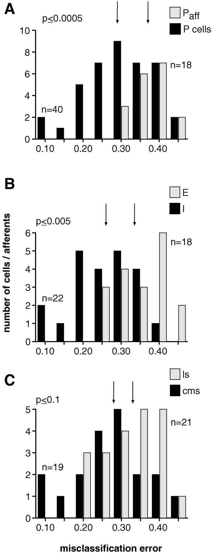
Comparison of the performance of different pyramidal cell types in various ELL maps and, in A only, of P-receptor afferents in the feature extraction task. A, Histogram of the best (lowest value across all stimulus presentations) misclassification error ε obtained for P-receptor afferents (P_aff; n = 18) and both types of pyramidal cells (P cells; n = 40; only spikes belonging to bursts are taken into account). Median value of distribution for P-receptor afferents (ε_median = 0.37) and for pyramidal cells (ε_median = 0.29) are indicated by the right and left vertical arrow, respectively. Higher values of the misclassification error indicate worse performance. The difference in median values is significant at the p ≤ 0.0005 level (Wilcoxon rank sum test).B, Distributions of the misclassification error for E-type (n = 18) and I-type pyramidal cells (n= 22) from both CMS and LS combined. Median value of distribution for I-units: ε_median = 0.26 (left vertical arrow) and for E-units: ε_median = 0.34 (right vertical arrow). Significance level: p ≤ 0.005.C, Distribution of the probability of misclassification for both E- and I-type pyramidal cells combined from LS (n= 21) versus those from CMS (n = 19). Median value of distribution for cells in CMS: ε_median = 0.28 (left vertical arrow) and for cells in LS: ε_median = 0.33 (right vertical arrow). Significance level: p ≤ 0.1.

Differences in feature extraction across pyramidal cell types and maps of the ELL

We investigated differences in the encoding of RAM up- and downstrokes among the various classes of ELL pyramidal cells from CMS and LS. We considered only those spikes that belonged to bursts because those encoded RAM up- and downstrokes best. By pooling I-type cells from CMS and LS and comparing their performance with E-type cells of the same segments, we found that I-type cells conveyed more accurately the presence of downstrokes than E-type cells encoded upstrokes (Fig.11B). Similarly, pyramidal cells in CMS extracted the temporal features in RAMs better than cells in LS (Fig.11C). The latter difference, however, was only significant at the p ≤ 0.1 level, and correspondingly, the overlap between the two distributions of misclassification errors was larger than between those of E- and I-type cells.

To further characterize the differences observed between E- and I-type pyramidal cells, pyramidal cells from CMS and LS, and pyramidal cells and P-receptor afferents, we performed pairwise comparisons among all possible classes of pyramidal cells and P-receptor afferents. The results are summarized in Table 1. The performance in the signaling of temporal features by the different cell classes inferred from Table 1 can be summarized by the following inequality (performance increased from left to right):

$$P_{\text{aff}}\ge E_{\text{ls}}\ge E_{\text{cms}}>I_{\text{ls}}>I_{\text{cms}}.$$ Equation 10

In Equation 10, the symbol X > Yindicates that the median misclassification error for cell class X was significantly larger than for cell class Y; or in other words, class Y performed the feature extraction task better than class X. On the other hand, the symbol X ≥ Y indicates that direct comparison between X and Y was not statistically significant and that the ordering was obtained by indirect comparisons with additional cell classes. Therefore, I-type pyramidal cells, especially those in CMS, extracted stimulus features better than E-type cells from either CMS or LS. In addition, the overlap between the distributions of misclassification errors of P-receptor afferents and pyramidal cells (Fig. 11A) is attributable largely to E-type pyramidal cells from LS (E_ls), whereas the overlap observed between pyramidal cells from CMS and LS (Fig.11C) resulted from pooling subgroups having intertwined performances (such as E_cms > I_ls > I_cms). The observed differences between pyramidal cells from CMS versus LS correlated with the different behavioral significance of ELL maps as discussed below.

Table 1.

Comparison of the performance of the two pyramidal cell types from CMS and LS as well as P-receptor afferents in the feature extraction task

	Paff	Els	Ecms	Ils	Icms
ɛmedian	0.37	0.38	0.30	0.29	0.23
n	18	9	9	12	10
Paff	↗	≈	>0.05	>0.0005	>0.0005
Els			≈	>0.01	>0.0005
Ecms				>0.1	>0.005
Ils					>0.05

First row: median value of the misclassification error, ɛ_median (for pyramidal cells, only spikes belonging to bursts were included). For each unit, only the best ɛ value was retained. Second row: number of analyzed units in each class. Remaining rows: results of pairwise comparisons of the median misclassification errors between all classes. Each class X (columns: P_aff, E_ls, E_cms, I_ls) was compared with each class Y (rows: E_ls, E_cms, I_ls, I_cms). The relation X ≈ Y indicates that differences were not statistically significant (p > 0.1). The relation X > Y symbolizes that the misclassification error for class X was larger than for Y, with the significance level shown underneath. In each column, note the monotone increase of the significance level from top to bottom, and in each row, the monotone decrease from left to right. This information was used to derive Equation 6 in the main text.

Encoding of RAM downstrokes in P-receptor afferent spike trains during periods of nonspiking

Downstrokes in RAMs of an electric field were encoded in P-receptor afferents by periods of nonspiking (Fig. 7A). We tested whether this information, when inverted by inhibitory interneurons in the granule cell layer of the ELL (Fig. 1) and consequently resulting in the lack of inhibitory input, could at least partly account for the good feature extraction found in I-type pyramidal cells. For this purpose, we applied feature extraction techniques to study the separation between 300-msec-long stretches of RAMs eliciting no spikes within their last 50 msec (between 250 and 300 msec of the stimulus waveform) and those eliciting at least one spike. This duration of 300 msec corresponds to the presumed integration time of pyramidal cells, as determined previously (Gabbiani et al., 1996). The corresponding feature vector was a downstroke in the amplitude modulation, and the separation between the two distributions was very good (ε = 0.08 ± 0.03; mean ± SD; n = 38 experiments on 18 P-receptor afferents). This suggested that periods of nonspiking or “silence” in P-receptor afferent spike trains were, indeed, reliable indicators of RAM downstrokes and could be used by I-type pyramidal cells to extract their optimal stimulus feature.

DISCUSSION

The electrosensory system in weakly electric fish provides the unique opportunity to combine computational and neuroethological approaches to quantify the information transfer from the sensory periphery to higher order central neurons in a sensory system the elements of which have a well characterized functional and behavioral significance (Maler, 1996). When pre- and postsynaptic responses to the same stimulus in this in vivo preparation were compared, our data suggest a substantial transformation in the encoding pattern of sensory signals between the first two stages of the amplitude coding pathway.

Computational methods

Linear stimulus estimation techniques by now have been applied to various neuronal preparations (Haag and Borst, 1997; for review, seeJohnson, 1996, Sec 3; Rieke et al., 1996, Chap 2; Gabbiani and Koch, 1998, Sec 9.7). They are well suited to identify the encoding of time-varying stimuli in neuronal spike trains and to quantify their accuracy, provided that the bandwidth of the stimulus is significantly lower than the firing rate of the neuron (Gabbiani and Koch, 1996;Johnson, 1996). This prerequisite was well satisfied by P-receptor afferents, enabling them to accurately encode low cut-off frequency time-varying amplitude modulations (AMs) (Fig. 7A) such as those expected to be behaviorally relevant for these animals (<80 Hz) (Bastian, 1981b). In contrast, the lower sustained discharge rates of pyramidal cells were less appropriate to transmit time-varying information about AMs (Fig. 8A–C). Nonetheless, this did not rule out the possibility that interactions between close pyramidal cell spikes, such as those belonging to bursts, could result in nonlinear encoding of time-varying stimuli. The relatively poor performance of nonlinear decoding techniques (Fig.8D), however, failed to support this idea. Therefore, pyramidal cell spike bursts appear not to be well suited to encode time-varying signals. This could be attributable partly to the relatively stereotyped length of their intraburst interspike intervals (Fig. 6) (Turner et al., 1996). Moreover, in this and previous studies (Wessel et al., 1996; Gabbiani et al., 1996), we exposed the entire body surface to RAMs, whereas under natural conditions only small regions of the receptor array are exposed to RAMs. Because our stimuli simultaneously activated the antagonistically organized center and surround of the receptive fields of pyramidal cells, this might have resulted in an underestimation of their performance.

Reliable stimulus estimation requires high sampling rates of the stimulus and a tuning of interspike intervals to stimulus intensity. In contrast, to reliably convey the presence of upstrokes or downstrokes in a random signal, spikes or spike bursts need to occur with a constant time lag to those features. In our study, the accuracy of feature encoding was assessed by the misclassification error of two pattern classifiers designed to discriminate between the distributions of stimuli that occurred before a spike and no spike, respectively. This involved the computation of first, the mean stimulus prior to a spike, which is the reverse-correlation between the stimulus and the spike train, second, the mean stimulus before no spike occurrence, and finally, the covariance matrices of both distributions. Thus, these methods could be regarded as a generalization of the reverse-correlation technique, extending it by characterizing the separation between stimuli occurring before a spike and no spike, respectively. This represents the novel aspect of our analysis technique. Because the two classifiers used in this study resulted in only small differences, we could have used the Euclidian classifier (which is considerably easier to compute) throughout our data analysis. Different random stimuli, such as nonstationary signals, might yield larger performance differences between them.

Methods of statistical pattern recognition have been applied previously to characterize the encoding of information in neuronal spike trains; for example, to categorize presented stimuli from neuronal responses (Becker and Krueger, 1996; Victor and Purpura, 1996; Middlebrooks et al., 1994).

Spontaneous activity of pyramidal cells in vivo andin vitro

The statistical properties of the spontaneous activity of pyramidal cells has also been characterized in a slice preparation of the ELL in the closely related Apteronotus (Turner et al., 1996). However, there were differences with our results obtained fromin vivo recordings in Eigenmannia. The CVs of the ISI distributions, for instance, were higher in the in vitrorecordings than in our study. Furthermore, the average values observedin vitro increased from LS to CMS and were correlated with increasing oscillation periods in the sub- and suprathreshold activity of pyramidal cells from LS to CMS. Although we could not readily verify these results in our study (Fig. 6A, inset), such map-specific oscillatory tuning might underlie the frequency tuning observed in vivo in response to sinusoidal AMs (Shumway, 1989). In our data sample, the range of CV values corresponded well with that reported from in vivo studies of other sensory systems (Teich et al., 1996). The absence of oscillations in vivo might be based on the presence of considerable feedforward and feedback synaptic inputs that are lacking in the slice preparation. In the mammalian neocortex, oscillatory discharge activity has also been observed more readily in vitro than in vivo(Silva et al., 1991).

Information processing between the first two stages of the amplitude pathway

This and previous investigations indicate that P-receptor afferents faithfully encode RAMs without substantial processing, except possibly for high-pass filtering (Bastian, 1981a; Gabbiani et al., 1996; Wessel et al., 1996). In this respect, they might be compared with simple analog-to-digital converters with binary output (Aziz et al., 1996; Gray, 1996). At the level of the subsequent stage, the ELL, most of this information is discarded in favor of an explicit representation of RAM upstrokes and downstrokes by short bursts of spikes. Part of this information is already present, although not explicitly, in the periods of nonspiking of P-receptor afferents that reliably encoded RAM downstrokes. Other studies have also emphasized the importance of spike bursts as units of information (Cattaneo et al., 1981; Crick, 1984; Otto et al., 1991; Bair et al., 1994; Lewicki and Konishi, 1995; Livingstone et al., 1996; for review, see Lisman, 1997).

Based on an estimate of the variance of ISI distributions, Bastian (1981b) determined that pyramidal cells were approximately 16 times more “effective” than receptor afferents in signaling changes in stimulus amplitude. Bastian (1986b) suggested that this might be attributable to convergence of afferent information, which is supported by anatomical observations (Carr et al., 1982).

Although the biophysical mechanisms responsible for the extraction of RAM upstrokes and downstrokes by pyramidal cells remain to be elucidated, they are most likely not based on a simple linear thresholding of the somatic membrane potential (Gabbiani et al., 1996). Several nonlinearities, including the active backpropagation of Na⁺ spikes from the proximal dendrites of pyramidal cells to their soma, could provide a physiological basis for this feature extraction (Turner et al., 1994). In addition, pyramidal cells receive massive efferent feedback projections, both excitatory and inhibitory, from higher order electrosensory structures that terminate primarily on their large apical dendrites (Bastian, 1986a; Carr and Maler, 1986; Bratton and Bastian, 1990; Maler and Mugnaini, 1994). Recently, it has been found in vitro that simultaneous input from one particular excitatory feedback circuit, the stratum fibrosum, and P-receptor afferents could greatly enhance the feedback input and become very effective in bringing the cell above spike threshold (Berman et al., 1997).

Earlier studies investigating the response properties of pyramidal cells used either sinusoidal or step-wise AMs. Bastian (1981a,b) reported that both E- and I-type pyramidal cells showed band-pass characteristics in their responses to variations in the frequency of sinusoidal AMs. He found that E-type pyramidal cells, much like P-type afferents, had peak responses for sinusoidal AMs around 64 Hz, whereas I-type pyramidal cells responded best to lower AMs (2–32 Hz). In contrast, Shumway (1989) reported no obvious differences between E- and I-units within a given map but described differences between the various maps. Most cells in the LS were characterized as high-pass filters, whereas most cells from the CMS were described as low-pass filters.

In response to RAM stimuli, most of the cells in our sample showed band-pass behavior (Figs. 4F, 7B,C). However, the peak frequency characterizing this band-pass behavior was not clearly correlated with the ELL map (CMS vs LS) or with the cell type (E- vs I-unit). Frequencies of the peak signal-to-noise ratios typically increased with the cut-off frequency of the stimulus. This suggests that the frequency tuning of pyramidal cells is stimulus dependent, as has been observed in vivo and in vitro in mammalian visual cortex (Reid et al., 1992; Carandini et al., 1996).

Differences in the extraction of temporal features across pyramidal cell types and maps of the ELL

Our results revealed differences in the encoding of RAM upstrokes and downstrokes between E- and I-type pyramidal cells (Figs. 9,11B) as well as between cells from CMS and LS (Fig.11C). In particular, I-type pyramidal cells from CMS performed the temporal feature extraction task best (Table 1). Previous investigations also showed differences in the encoding of brief temporal modulations of signal amplitude between E- and I-units (Metzner and Heiligenberg, 1991). The homogeneous electric field geometry used in this study is expected to maximally activate the inhibitory commissural connections terminating on E-type pyramidal cells responsible for common mode rejection (Bastian and Courtright, 1991; Bastian et al., 1993; Maler and Mugnaini, 1994). This might explain the lower performance of E-units as compared with I-units. Stimulation localized within the receptive fields of individual E- and I-units will have to be used to test this hypothesis.

Various physiological differences between the two ELL maps, CMS and LS, have been described previously (Shumway, 1989; Metzner and Heiligenberg, 1991; Turner et al., 1996). Their functional significance might be concluded from results derived from recent inactivation studies that revealed distinctly different behavioral significances for CMS and LS, respectively (Metzner and Juranek, 1997). The CMS was necessary and sufficient for the processing of signals eliciting a particular electrolocative behavior, the jamming avoidance response, whereas the LS was necessary and sufficient to process signals that evoke communication behavior. Whereas the pattern that evokes chirping in Eigenmannia might be more complex and involve extreme low-frequency modulations of the baseline voltage of the signal (Metzner and Heiligenberg, 1991), up- and downstrokes of AMs are an integral part of the stimulus pattern yielding a jamming avoidance response (Heiligenberg, 1991).

In conclusion, the present study demonstrates not only that a significant transformation in the signal processing mode can already occur between the first two stages of a sensory pathway, but it also exemplifies how a combination with neuroethological findings enriches the interpretation of results from information theoretical approaches and helps to clarify their functional and behavioral significance. Future studies will expand this combined approach to study the encoding of spatially localized and thus more natural stimuli, as well as simultaneous encoding in multiple pyramidal cell spike trains with overlapping receptive fields.

REFERENCES

- 1.Anderson TW. An introduction to multivariate statistical analysis, Ed 2. Wiley; New York: 1984. [Google Scholar]
- 2.Anderson TW, Bahadur RR. Classification into two multivariate normal distributions with different covariance matrices. Ann Math Stat. 1962;33:420–431. [Google Scholar]
- 3.Aziz PM, Sorensen HV, Van der Spiegel J. An overview of sigma-delta converters. IEEE Sig Proc Mag. 1996;13:61–84. [Google Scholar]
- 4.Bair W, Koch C, Newsome W, Britten K. Power spectrum analysis of bursting cells in area MT in the behaving monkey. J Neurosci. 1994;14:2870–2892. doi: 10.1523/JNEUROSCI.14-05-02870.1994. [DOI] [PMC free article] [PubMed] [Google Scholar]
- 5.Bastian J. Electrolocation: I. The effects of moving objects and other electric stimuli on the activities of two categories of posterior lateral line cells in Apteronotus albifrons. J Comp Physiol. 1981a;144:481–494. [Google Scholar]
- 6.Bastian J. Electrolocation: II. How the electroreceptors of Apteronotus albifrons code for moving objects and other electric signal. J Comp Physiol. 1981b;144:465–479. [Google Scholar]
- 7.Bastian J. Gain control in the electrosensory system mediated by descending inputs to the electrosensory lateral line lobe. J Neurosci. 1986a;6:553–562. doi: 10.1523/JNEUROSCI.06-02-00553.1986. [DOI] [PMC free article] [PubMed] [Google Scholar]
- 8.Bastian J. Electrolocation. In: Bullock TH, Heiligenberg W, editors. Electroreception. Wiley; New York: 1986b. pp. 577–612. [Google Scholar]
- 9.Bastian J. Electrosensory organisms. Phys Today. 1994;47:30–37. [Google Scholar]
- 10.Bastian J, Courtright J. Morphological correlates of pyramidal cell adaptation rate in the electrosensory lateral line lobe of weakly electric fish. J Comp Physiol [A] 1991;168:393–407. doi: 10.1007/BF00199600. [DOI] [PubMed] [Google Scholar]
- 11.Bastian J, Heiligenberg W. Neural correlates of the jamming avoidance response of Eigenmannia. J Comp Physiol. 1980;136:135–152. doi: 10.1126/science.7403849. [DOI] [PubMed] [Google Scholar]
- 12.Bastian J, Courtright J, Crowford J. Commisural neurons of the electrosensory lateral line lobe of Apteronotus leptorhynchus: morphological and physiological characteristics. J Comp Physiol. 1993;173:257–274. doi: 10.1007/BF00212690. [DOI] [PubMed] [Google Scholar]
- 13.Becker JD, Krueger J. Recognition of visual stimuli from multiple neuronal activity in monkey visual cortex. Biol Cybern. 1996;74:287–298. doi: 10.1007/BF00194921. [DOI] [PubMed] [Google Scholar]
- 14.Berman NJ, Plant J, Turner RW, Maler L. Excitatory amino acid receptors at a feedback pathway in the electrosensory system: implications for the searchlight hypothesis. J Neurophysiol. 1997;78:1869–1881. doi: 10.1152/jn.1997.78.4.1869. [DOI] [PubMed] [Google Scholar]
- 15.Bialek W, de Ruyter van Steveninck R, Warland D. Reading a neural code. Science. 1991;252:1854–1857. doi: 10.1126/science.2063199. [DOI] [PubMed] [Google Scholar]
- 16.Bishop CM. Neural networks for pattern recognition. Clarendon Press; Oxford: 1995. [Google Scholar]
- 17.Bratton B, Bastian J. Descending control of electroreception: II. Properties of nucleus praeeminentialis neurons projecting directly to the electrosensory lateral line lobe. J Neurosci. 1990;10:1241–1253. doi: 10.1523/JNEUROSCI.10-04-01241.1990. [DOI] [PMC free article] [PubMed] [Google Scholar]
- 18.Carandini M, Mechler F, Leonard CS, Movshon JA. Spike train encoding by regular-spiking cells of the visual cortex. J Neurophysiol. 1996;76:3425–3441. doi: 10.1152/jn.1996.76.5.3425. [DOI] [PubMed] [Google Scholar]
- 19.Carr CE, Maler L. Electroreception in gymnotiform fish, central anatomy and physiology. In: Bullock TH, Heiligenberg W, editors. Electroreception. Wiley; New York: 1986. pp. 319–373. [Google Scholar]
- 20.Carr CE, Maler L, Sas E. Peripheral organization and central projections of the electrosensory nerves in gymnotiform fish. J Comp Neurol. 1982;211:139–153. doi: 10.1002/cne.902110204. [DOI] [PubMed] [Google Scholar]
- 21.Cattaneo A, Maffei L, Morrone C. Two firing patterns in the discharge of complex cells encoding different attributes of the visual stimulus. Exp Brain Res. 1981;43:115–118. doi: 10.1007/BF00238819. [DOI] [PubMed] [Google Scholar]
- 22.Crick F. Function of the thalamic reticular complex: the searchlight hypothesis. Proc Natl Acad Sci USA. 1984;81:4586–4590. doi: 10.1073/pnas.81.14.4586. [DOI] [PMC free article] [PubMed] [Google Scholar]
- 23.Efron B. The efficiency of logistic regression compared to normal discriminant analysis. J Am Stat Assoc. 1975;70:892–898. [Google Scholar]
- 24.Enger PS, Szabo T. Activity of central neurons involved in electroreception in some weakly electric fish (Gymnotidae). J Neurophysiol. 1965;28:800–818. doi: 10.1152/jn.1965.28.5.800. [DOI] [PubMed] [Google Scholar]
- 25.Fortune ES, Rose GJ. Passive and active membrane properties contribute to the temporal filtering properties of midbrain neurons in vivo. J Neurosci. 1997;17:3815–3825. doi: 10.1523/JNEUROSCI.17-10-03815.1997. [DOI] [PMC free article] [PubMed] [Google Scholar]
- 26.Fukunaga K. Introduction to statistical pattern recognition, Ed 2. Academic; San Diego: 1990. [Google Scholar]
- 27.Gabbiani F, Koch C. Coding of time-varying signals in spike trains of integrate-and-fire neurons with random threshold. Neural Comput. 1996;8:44–66. [Google Scholar]
- 28.Gabbiani F, Koch C. Principles of spike train analysis. In: Koch C, Seguev I, editors. Methods in neuronal modeling, Ed 2. MIT; Cambridge, MA: 1998. pp. 313–360. [Google Scholar]
- 29.Gabbiani F, Metzner W, Wessel R, Koch C. From stimulus encoding to feature extraction in weakly electric fish. Nature. 1996;384:564–567. doi: 10.1038/384564a0. [DOI] [PubMed] [Google Scholar]
- 30.Gray RM. Quantization noise in sigma-delta A/D converters. In: Norsworthy S, Schreier R, Themes G, editors. Delta-sigma data converters: theory, design and simulations. IEEE Press; Piscataway, NJ: 1996. pp. 44–74. [Google Scholar]
- 31.Green D, Swets J. Signal detection theory and psychophysics. Wiley; New York: 1966. [Google Scholar]
- 32.Greenander U, Szegö G. Toeplitz forms and their applications. University of California; Berkley, CA: 1958. [Google Scholar]
- 33.Haag J, Borst A. Encoding of visual motion information and reliability in spiking and graded potential neurons. J Neurosci. 1997;17:4809–4819. doi: 10.1523/JNEUROSCI.17-12-04809.1997. [DOI] [PMC free article] [PubMed] [Google Scholar]
- 34.Hamming RW. Digital filters, Ed 3. Prentice Hall; Englewood Cliffs, NJ: 1989. [Google Scholar]
- 35.Heiligenberg W. Neural nets in electric fish. MIT; Cambridge MA: 1991. [Google Scholar]
- 36.Heiligenberg . Electrosensation. In: Evans DH, editor. The physiology of fishes. CRC; Boca Raton, FL: 1993. pp. 137–160. [Google Scholar]
- 37.Heiligenberg W, Dye J. Labeling of electroreceptive afferents in a gymnotoid fish by intracellular injection of HRP: the mystery of multiple maps. J Comp Physiol. 1982;148:287–296. [Google Scholar]
- 38.Heiligenberg W, Metzner W, Wong CJH, Keller CH. Motor control of the jamming avoidance response of Apteronotus leptorhynchus: evolutionary changes of a behavior and its neuronal substrates. J Comp Physiol [A] 1996;179:653–674. doi: 10.1007/BF00216130. [DOI] [PubMed] [Google Scholar]
- 39.Johnson DH. Point process models of single-neuron discharges. J Comput Neurosci. 1996;3:275–299. doi: 10.1007/BF00161089. [DOI] [PubMed] [Google Scholar]
- 40.Jolliffe IT. Principal component analysis. Springer; New York: 1986. [Google Scholar]
- 41. Koch C. Biophysics of computation: information processing in single neurons. 1998. Oxford UP; Oxford, in press. [Google Scholar]
- 42.Koh T, Powers EJ. Second-order volterra filtering and its application to nonlinear system identification. IEEE Trans Acoust Speech Signal Proc. 1985;33:1445–1455. [Google Scholar]
- 43.Konishi M. Deciphering the brain’s codes. Neural Comput. 1991;3:1–18. doi: 10.1162/neco.1991.3.1.1. [DOI] [PubMed] [Google Scholar]
- 44.Korenberg MJ. Identifying nonlinear difference equation and functional expansion representations: the fast orthogonal algorithm. Ann Biomed Eng. 1988;16:123–142. doi: 10.1007/BF02367385. [DOI] [PubMed] [Google Scholar]
- 45.Lehmann EL. Nonparametrics: statistical methods based on ranks. Holden-Day; San Francisco: 1975. [Google Scholar]
- 46.Lewicki MS, Konishi M. Mechanisms underlying the sensitivity of songbird forebrain neurons to temporal order. Proc Natl Acad Sci USA. 1995;92:5582–5586. doi: 10.1073/pnas.92.12.5582. [DOI] [PMC free article] [PubMed] [Google Scholar]
- 47.Lisman JE. Bursts as a unit of neural information: making unreliable synapses reliable. Trends Neurosci. 1997;20:38–43. doi: 10.1016/S0166-2236(96)10070-9. [DOI] [PubMed] [Google Scholar]
- 48.Livingstone MS, Freeman DC, Hubel DH. Visual responses in V1 of freely viewing monkeys. Cold Spring Harbor Symp Quant Biol. 1996;6:27–37. [PubMed] [Google Scholar]
- 49.Maler L. The posterior lateral line lobe of certain gymnotiform fish: quantitative light microscopy. J Comp Neurol. 1979;183:323–363. doi: 10.1002/cne.901830208. [DOI] [PubMed] [Google Scholar]
- 50.Maler L. The role of feedback pathways in the modulation of receptive fields: an example from the electrosensory system. In: Erber J, Menzel R, Pfluger HJ, Todt D, editors. Neural mechanisms of behavior, Proceedings of the 2nd International Congress on Neuroethology. Thieme; New York: 1989. pp. 111–115. [Google Scholar]
- 51.Maler L. Train signals for electric fish. Nature. 1996;384:517–518. doi: 10.1038/384517a0. [DOI] [PubMed] [Google Scholar]
- 52.Maler L, Mugnaini E. Correlating gamma-aminobutyric acidergic circuits and sensory function in the electrosensory lateral line lobe of a Gymnotiform fish. J Comp Neurol. 1994;345:224–252. doi: 10.1002/cne.903450206. [DOI] [PubMed] [Google Scholar]
- 53.Maler L, Sas E, Johnston S, Ellis W. An atlas of the brain of the electric fish Apteronotus leptorhynchus. J Chem Neuroanat. 1991;4:1–38. doi: 10.1016/0891-0618(91)90030-g. [DOI] [PubMed] [Google Scholar]
- 54.Marmarelis PZ, McCann GD. Development and application of white-noise modeling techniques for studies of insect visual nervous systems. Kybernetik. 1973;12:74–89. doi: 10.1007/BF00272463. [DOI] [PubMed] [Google Scholar]
- 55.Marmarelis PZ, Naka KI. White noise analysis of a neuron chain: an application of the Wiener theory. Science. 1972;175:1276–1278. doi: 10.1126/science.175.4027.1276. [DOI] [PubMed] [Google Scholar]
- 56.Marr D. Vision. Freeman; New York: 1982. [Google Scholar]
- 57.Mathieson WB, Maler L. Morphological and electrophysiological properties of a novel in vitro preparation: the electrosensory lateral line lobe brain slice. J Comp Physiol. 1988;163:489–506. doi: 10.1007/BF00604903. [DOI] [PubMed] [Google Scholar]
- 58.Metzner W. The jamming avoidance response in Eigenmannia is controlled by two separate motor pathways. J Neurosci. 1993;13:1862–1878. doi: 10.1523/JNEUROSCI.13-05-01862.1993. [DOI] [PMC free article] [PubMed] [Google Scholar]
- 59.Metzner W, Heiligenberg W. The coding of signals in the electric communication of the gymnotiform fish Eigenmannia: from electroreceptors to neurons in the torus semicircularis of the midbrain. J Comp Physiol [A] 1991;169:135–150. doi: 10.1007/BF00215861. [DOI] [PubMed] [Google Scholar]
- 60.Metzner W, Viete S. The neuronal basis of communication and orientation in the weakly electric fish Eigenmannia 1. Communication behavior or seeking a conspecifics response. Naturwissenschaften. 1996a;83:6–14. [Google Scholar]
- 61.Metzner W, Viete S. The neuronal basis of communication and orientation in the weakly electric fish Eigenmannia 1. Electrolocation and avoidance of jamming by neighboring conspecifics. Naturwissenschaften. 1996b;83:71–77. [Google Scholar]
- 62.Metzner W, Juranek J. A sensory brain map for each behavior? Proc Natl Acad Sci USA. 1997;94:14798–14803. doi: 10.1073/pnas.94.26.14798. [DOI] [PMC free article] [PubMed] [Google Scholar]
- 63.Middlebrooks JC, Clock AE, Xu L, Green D. A panoramic code for sound location by cortical neurons. Science. 1994;264:842–844. doi: 10.1126/science.8171339. [DOI] [PubMed] [Google Scholar]
- 64.Oppenheim AV, Schafer RW. Discrete signal processing. Prentice Hall; Englewood Cliffs, NJ: 1989. [Google Scholar]
- 65.Otto T, Eichenbaum H, Wiener SI, Wible CG. Learning-related patterns of CA1 spike trains parallel stimulation parameters optimal for inducing hippocampal long-term potentiation. Hippocampus. 1991;1:181–192. doi: 10.1002/hipo.450010206. [DOI] [PubMed] [Google Scholar]
- 66.Poor HV. An introduction to signal detection and estimation, Ed 2. Springer; New York: 1994. [Google Scholar]
- 67.Press WH, Teukolsky SA, Vetterling WT, Flannery BP. Numerical recipes in C, Ed 2. Cambridge UP; Cambridge, MA: 1992. [Google Scholar]
- 68.Raudys SJ, Jain AK. Small sample size effects in statistical pattern recognition: recommendations for practitioners. IEEE Trans Patt Anal Mach Int. 1991;13:252–264. [Google Scholar]
- 69.Reichardt W, Poggio T. Visual control of orientation behavior in the fly. Part I. A quantitative analysis. Q Rev Biophys. 1976;9:311–375. doi: 10.1017/s0033583500002523. [DOI] [PubMed] [Google Scholar]
- 70.Reid RC, Victor JD, Shapley RM. Broadband temporal stimuli decrease the integration time of neurons in cat striate cortex. Vis Neurosci. 1992;9:39–45. doi: 10.1017/s0952523800006350. [DOI] [PubMed] [Google Scholar]
- 71.Rieke F, Warland D, de Ruyter van Steveninck R, Bialek W. Spikes, exploring the Neural Code. MIT; Cambridge, MA: 1996. [Google Scholar]
- 72.Rose GJ, Call SJ. Evidence for the role of dendritic spines in the temporal filtering properties of neurons: the decoding problem and beyond. Proc Nat Acad Sci USA. 1992;89:9662–9665. doi: 10.1073/pnas.89.20.9662. [DOI] [PMC free article] [PubMed] [Google Scholar]
- 73.Rose GJ, Call SJ. Temporal filtering properties of midbrain neurons in an electric fish: implications for the function of dendritic spines. J Neurosci. 1993;13:1178–1189. doi: 10.1523/JNEUROSCI.13-03-01178.1993. [DOI] [PMC free article] [PubMed] [Google Scholar]
- 74.Saunders J, Bastian J. The physiology and morphology of two types of electrosensory neurons in the weakly electric fish Apteronotus leptorhynchus. J Comp Physiol [A] 1984;154:199–209. [Google Scholar]
- 75.Scheich H, Bullock TH, Hamstra RH. Coding properties of two classes of afferent nerve fibers: high frequency electroreceptors in the electric fish, Eigenmannia. J Neurophysiol. 1973;36:39–60. doi: 10.1152/jn.1973.36.1.39. [DOI] [PubMed] [Google Scholar]
- 76.Shumway C. Multiple electrosensory maps in the medulla of weakly electric gymnotiform fish. I. Physiological differences. J Neurosci. 1989;9:4388–4399. doi: 10.1523/JNEUROSCI.09-12-04388.1989. [DOI] [PMC free article] [PubMed] [Google Scholar]
- 77.Silva LR, Amitai Y, Connors BW. Intrinsic oscillations of neocortex generated by layer 5 pyramidal neurons. Science. 1991;251:432–435. doi: 10.1126/science.1824881. [DOI] [PubMed] [Google Scholar]
- 78.Teich M, Turcott RG, Siegel RM. Temporal correlation in cat striate-cortex neural spike trains. IEEE Eng Med Biol Mag. 1996;15:79–87. [Google Scholar]
- 79.Turner RW, Maler L, Deerinck T, Levinson SR, Ellisman MH. TTX-sensitive dendritic sodium channels underlie oscillatory discharge in a vertebrate sensory neuron. J Neurosci. 1994;14:6453–6471. doi: 10.1523/JNEUROSCI.14-11-06453.1994. [DOI] [PMC free article] [PubMed] [Google Scholar]
- 80.Turner RW, Plant JR, Maler L. Oscillatory and burst discharges across electrosensory topographic maps. J Neurophysiol. 1996;76:2364–2382. doi: 10.1152/jn.1996.76.4.2364. [DOI] [PubMed] [Google Scholar]
- 81.Victor JD, Purpura KP. Nature and precision of temporal coding in visual cortex: a metric-space analysis. J Neurophysiol. 1996;76:1310–1326. doi: 10.1152/jn.1996.76.2.1310. [DOI] [PubMed] [Google Scholar]
- 82.Wessel R, Koch C, Gabbiani F. Coding of time-varying electric field amplitude modulations in a wave-type electric fish. J Neurophysiol. 1996;75:2280–2293. doi: 10.1152/jn.1996.75.6.2280. [DOI] [PubMed] [Google Scholar]
- 83.Zakon HH. The electroreceptive periphery. In: Bullock TH, Heiligenberg W, editors. Electroreception. Wiley; New York: 1986. pp. 103–156. [Google Scholar]