Active Membrane Properties and Signal Encoding in Graded Potential Neurons

Abstract

We investigated the influence of active membrane properties on the precision by which the stimulus velocity is encoded in the membrane potential of a motion-sensitive interneuron in the blowfly. The so-called HS-cells respond to visual motion stimuli with a graded shift in membrane potential. Superimposed on this graded response are small spike-like events. This “mixed” visual response mode can be modified by current injection in two different ways. (1) By ongoing injection of hyperpolarizing current, the spike-like events are turned into full-blown action potentials, and (2) by injection of depolarizing current, the spike-like events become completely suppressed. The visual response then consists of a graded shift of membrane potential only. As a measure of the fidelity, we calculated the coherence between the motion stimulus and the response of the cell elicited with different electrical manipulations of the cell. We found that the coherence was highest for the cell at rest. Any electrical manipulation resulted in a reduced coherence. This was attributable partly to a lower signal-to-noise ratio and partly to an increased nonlinearity in the response. By applying a threshold operation we transformed the analog membrane response into an all-or-none spike train. A comparison between these two ways of signal representation revealed that more information about the stimulus velocity is inherent in the analog membrane potential than in the spike train.

Most neurons communicate with each other by sending trains of action potentials along their axons. However, in addition to these classical spiking neurons, another type of nerve cells called “graded potential neurons” is found in various parts of the nervous system in vertebrates as well as in invertebrates. In contrast to the former, graded potential neurons usually do not produce regular action potentials but rather shift their membrane potential in a graded way according to the prevalent input signal.

A long-standing problem concerning these graded potential neurons is the question of what difference exists between them and spiking neurons with respect to the information they convey about the input signal (Bullock, 1981). Is the graded mode more reliable than the spiking mode? Can graded neurons carry more information than spiking ones or the other way around? We examined this question previously by comparing signal encoding in spiking (H1-cells) and graded potential neurons (HS-cells) of the fly visual system (Haag and Borst, 1997). Both neurons belong to the class of lobula plate tangential cells (LPTCs), located in the posterior part of the third visual neuropile (lobula plate) of the blowfly, which are known to respond to visual motion stimuli in a directionally selective way (Borst and Egelhaaf, 1989,1990; Egelhaaf et al., 1989). H1-cells communicate between the lobula plates of both hemispheres by sending trains of action potentials along their axons. HS-cells synapse onto descending neurons and respond to visual motion by a graded shift of their axonal membrane potential (Hausen, 1982a, 1982b, 1984; Borst and Haag, 1996). Applying the so-called “reverse reconstruction technique” (Bialek et al., 1991;Bialek and Rieke, 1992; Theunissen, 1993; Gabbiani et al., 1996;Theunissen et al., 1996), we showed that the time-course of image velocity could be better retrieved from the graded signals of HS-cells than from the spike trains of H1-cells, the reason being the limited dynamic range of the spiking neuron for inhibitory stimuli attributable to the low spontaneous spike frequency (Haag and Borst, 1997). This might lead to the conclusion that a purely graded neuron without any active membrane properties could perform optimally in representing sensory information. However, despite their graded response to visual motion, HS-cells house various kinds of voltage-gated currents. Voltage-clamp experiments revealed that these cells show a fast sodium inward current that, depending on the resting state of their membrane potential, can lead to spike-like events superimposed on the graded shift of membrane potential (Borst and Haag, 1996; Haag et al., 1997). These active processes have been previously shown to enhance the cellular responses to high-frequency synaptic input signals (Haag and Borst, 1996). By additional manipulation of the resting membrane potential via injection of hyperpolarizing currents, these cells can be turned from their normal “mixed” visual response mode into almost purely spiking cells (Hengstenberg, 1997), or, alternatively, by injection of depolarizing current, into purely graded cells (Haag and Borst, 1996).

The analysis of the role of active membrane properties with respect to the information they convey might be of further interest because the dendrites of all neurons transmit signals mainly in a graded potential manner, and, as in HS-cells, many of them house various voltage-gated channels (Hirsch and Gilbert, 1991; Stuart and Sakmann, 1994; Yuste et al., 1994; Callaway and Ross, 1995; Spruston et al., 1995). The contribution of these active membrane properties to dendritic information processing is not yet fully understood (Yuste and Tank, 1996).

In the present study we compare the encoding of velocity information in HS-cells under various manipulations of their membrane potential and ask to what degree fast membrane processes contribute to a more accurate encoding as compared with a purely spiking or a purely graded response mode. This study thus aims at a functional understanding of the impact that active membrane processes have on neural coding in graded potential neurons. We will also investigate to what degree the usual resting potential of HS-cells represents an ideal set-point with respect to the signal-to-noise levels inherent in the cellular membrane signals.

MATERIALS AND METHODS

Preparation and set-up

Female blowflies (Calliphora erythrocephala) were briefly anesthesized with CO₂ and mounted ventral side up with wax on a small preparation platform. The head capsule was opened from behind; the trachea and airsacs that normally cover the lobula plate were removed. To eliminate movements of the brain caused by peristaltic contractions of the esophagus, the proboscis of the animal was cut away, and the gut was pulled out. This allowed stable intracellular recordings of up to 45 min. The fly was then mounted in an upright position on a heavy recording table with the stimulus monitors in front of the animal. The fly brain was viewed from behind through a Zeiss dissection scope.

Stimulation

Stimuli were generated on Tektronix 608 monitors by an image synthesizer (Picasso, Innisfree) and consisted of a one-dimensional grating of 14° spatial wavelength and 87% contrast displayed at a frame rate of 200 Hz. The mean luminosity of the screen was 11.2 cd/m². The intensity of the pattern was square-wave-modulated along its horizontal axis. The angular width of the stimulus fields was 40° in the horizontal and 28° in the vertical direction as seen by the fly. To identify the cells by their visual response properties, cells were first stimulated by the pattern moving back and forth at 28°/sec. When the actual experiment was started, the stimulus moved at a pseudo-random velocity with a flat spectrum up to 30–40 Hz (Fig. 1). The mean velocity of the stimulus was 0°/sec with a SD of 99.5°/sec. One stimulus sweep lasted for 40 sec, and a variable number of sweeps (5–10) were presented to each cell during one experiment. This was repeated for each current injection that was imposed on the cell via the recording electrode. Three levels were used, each of which turned the cell into a distinct response mode: 0, −3, and +3 nA. The injection of the hyperpolarizing current led to a potential shift of approximately −12 to −14 mV; the injection of depolarizing current led to a shift in membrane potential of approximately +10 mV.

Fig. 1.

Amplitude spectrum of the stimulus used for all experiments. The stimulus has a flat amplitude spectrum up to 30–40 Hz.

Recording

For intracellular recordings of HS-cells, electrodes were pulled on a Brown-Flaming micropipette puller (P-97) using thin-wall glass capillaries with an outer diameter of 1 mm (Clark, GC100TF-10). When filled with 1 m KCl they had resistances of ∼20 MΩ. A SEL10-amplifier (npi Electronics), which was operated in the bridge mode, was used throughout the experiments. Out of the three different HS-cells that are located in the lobula plate of each brain hemisphere (HSN-, HSE-, and HSS-cells) we recorded only from HSN- and HSE-cells. Because these cells, apart from their different receptive field locations, did not exhibit any differences in their response properties, data from both cell types were pooled and are collectively referred to as “HS-cells” in the following. All recordings were made in the axons of these cells. Extracellular recordings of H1-cells were made using standard tungsten electrodes with a resistance of ∼5 MΩ. Extracellular signals were bandpass-filtered and subsequently processed by a threshold device delivering a 100 mV pulse of 1 msec duration on each spike detected. For data analysis, the output signal of the threshold device as well as the stimulus function controlling the velocity of the pattern were fed to a PS/2 PC via a 12-bit A/D converter (Metra Byte μCDAS-16G, Keithley Instruments) at a sampling rate of 2 kHz and stored to hard disc.

Data evaluation

For theoretical background, also see Shannon and Weaver (1949),Cover and Thomas (1991), Theunissen (1993), Theunissen et al. (1996), and Rieke et al. (1997).

Reverse filter. Consider a stimulus S(t) that causes, by some unknown transformation, a response R(t). We want to estimate S(t) from R(t). To optimize the reconstruction one chooses the filter G_rev, which minimize the mean square error χ² between S(t) and S^est(t):

$${\chi }^2=\underset{T\to \infty }{\text{lim}} \frac{1}{T}\underset{0}{\overset{T}{\int }}(s(t)-s^{\text{est}}(t){)}^2\text{dt}.$$ Equation 1

Minimizing the mean square error leads to a filter G_rev. In the linear case the equation for this optimal filter can be solved in frequency space (with 〈 〉 denoting the average over different stretches of data S_iand R_i and * denoting the complex conjugate; see Implementation below):

$$G_{\text{rev}}(f)=\frac{\langle R_{\text{i}}*(f)·S_{\text{i}}(f)\rangle }{\langle R_{\text{i}}*(f)·R_{\text{i}}(f)\rangle }.$$ Equation 2

This filter represents, in frequency space, the average cross-correlation between stimulus and response divided by the average auto-correlation of the response. It is the slope of a linear regression for S_i– R_ipairs at each frequency.

Coherence function. The following section describes the calculation of the coherence function. On the basis of the signal-to-noise ratios (SNRs), we will also define and calculate an expected coherence function assuming that the system uses a linear encoding scheme. For evaluating the quality of the reconstruction, we calculate the gain relating S(t) to S^est(t).

This gain is defined as:

$${\gamma }^2(f)=\frac{\langle S_{\text{i}}*(f)·S_{\text{i}}^{\text{est}}(f)\rangle }{\langle S_{\text{i}}*(f)·S_{\text{i}}(f)\rangle }.$$ Equation 3

S^est(f) relates to R(f) and S(f) in the following way:

$$S_{\text{i}}^{\text{est}}(f)=R_{\text{i}}(f)·G_{\text{rev}}(f)=R_{\text{i}}(f)·\frac{\langle R_{\text{i}}*(f)·S_{\text{i}}(f)\rangle }{\langle R_{\text{i}}*(f)·R_{\text{i}}(f)\rangle }.$$ Equation 4

Inserting (4) into (3) yields:

$${\gamma }^2(f)=\frac{\langle S_{\text{i}}*(f)·R_{\text{i}}(f)\rangle }{\langle S_{\text{i}}*(f)·S_{\text{i}}(f)\rangle }·\frac{\langle R_{\text{i}}*(f)·S_{\text{i}}(f)\rangle }{\langle R_{\text{i}}*(f)·R_{\text{i}}(f)\rangle }.$$ Equation 5

This quantity, called the coherence γ², represents the product of the average cross-correlations between the stimulus and the response and vice versa, divided by the stimulus and response power. It can be also understood as the product of the optimal linear forward filter G_fwd transforming S into R, and the optimal linear reverse filter G_rev.

It follows from Equation 5 that 0 ≤ γ² ≤ 1.

The deviation of a measured coherence from 1 can be attributed to two different causes (1) the system is not linear; (2) the system is corrupted by noise. To disentangle these two possible sources, we calculated an expected coherence γ_exp²for a linear system.

Given a linear system that is corrupted by additive noise, R_i(f) = G_fwdS_i(f) + N_i(f), Equation 5 turns into:

$${\gamma }_{exp}^2(f)=\frac{\langle S_{\text{i}}*(f)·[G_{\text{fwd}}(f)·S_{\text{i}}(f)+N_{\text{i}}(f)]\rangle }{\langle S_{\text{i}}*(f)·S_{\text{i}}(f)\rangle }.$$

$$\frac{\langle [G_{\text{fwd}}*(f)·S_{\text{i}}*(f)+N_{\text{i}}*(f)]·S_{\text{i}}(f)\rangle }{\langle [G_{\text{fwd}}(f)·S_{\text{i}}*(f)+N_{\text{i}}*(f)]·[G_{\text{fwd}}(f)·S_{\text{i}}(f)+N_{\text{i}}(f)]\rangle }.$$

If the stimulus and the noise are uncorrelated 〈S_i(f)·N_i(f)〉 = 0, for all frequencies (f) this expression simplifies to:

$${\gamma }_{exp}^2(f)=\frac{\Vert G_{\text{fwd}}(f){\Vert }^2\langle S_{\text{i}}^{*}(f)S_{\text{i}}(f)\rangle }{\Vert G_{\text{fwd}}(f){\Vert }^2\langle S_{\text{i}}^{*}(f)S_{\text{i}}(f)\rangle +\langle N_{\text{i}}^{*}(f)N_{\text{i}}(f)\rangle }.$$ Equation 6

The signal-to-noise ratio is defined as the quotient of the signal and the noise power. Because the signal is the average response, i.e., the response without noise, this expression becomes:

$$SNR(f)=\frac{\langle \Vert G_{\text{fwd}}{\Vert }^2{S}_{\text{i}}^{*}(f)S_{\text{i}}(f)\rangle }{\langle N_{\text{i}}^{*}(f)N_{\text{i}}(f)\rangle }.$$ Equation 7

Combining Equations 6 and 7 yields:

$${\gamma }_{exp}^2(f)=\frac{SNR(f)}{SNR(f)+1}.$$ Equation 8

Thus, based on the measured SNR, we can assign an expected coherence γ_exp² to a system, assuming that it is linear and the stimulus and noise are uncorrelated. The expected coherence can be also written as the ratio of the power of the average response and the average power of the response. Comparing this expected with the actually measured coherence allows the difference 1 − γ² to split up into a part that is caused by noise (1 − γ_exp²) and another fraction that is caused by nonlinearity (γ_exp² − γ²).

Upper and lower bound of information rate. We will now show how the two terms introduced above, i.e., the measured coherence γ² and the coherence as expected for a linear system, γ_exp², given a certain signal-to-noise ratio SNR, relate to the lower and upper bound of the information rate in a neural signal, respectively.

If the mean response and the noise have a Gaussian distribution and are independent of each other, the upper bound or “channel capacity” can be calculated as:

$${\text{Info}}_{UB}(\text{bits}/sec)=\underset{f=0}{\overset{f=k}{\int }}{log}_2[1+SNR(f)]\text{df}.$$ Equation 9

By inserting Equation 8 into 9, one obtains:

$${\text{Info}}_{UB}(\text{bits}/sec)=-\underset{f=0}{\overset{f=k}{\int }} {log}_2[1-{\gamma }_{exp}^2(f)]\text{df}.$$ Equation 10

We now calculate the lower bound of the information rate. This calculation is based on the data processing inequality theorem, which says that no clever manipulation of R can increase the inference that can be made from R about S.

Given a processing chain S → R → S^est, then I(S, S^est) ≤ I(S, R).

Therefore we can safely transform the response R by whatever filter and will never overestimate the information in R about S. Hence it follows that the information in S^est about S will be a lower bound of the real information that is in R about S. We define a signal-to-noise ratio of our reconstruction,SNR_Rec, as the mean power ratio of S^est and the difference between S and S^est:

$${SNR}_{\text{Rec}}(f)=\frac{\langle S^{\text{est}}*(f)·S^{\text{est}}(f)\rangle }{\langle (S(f)-S^{\text{est}}(f))*·(S(f)-S^{\text{est}}(f))\rangle }.$$ Equation 11

This expression is identical to the one used by Rieke et al. (1997) who defined SNR_Rec as the mean power ratio of the stimulus and the difference between S and S^est/γ². Combining Equations 4 and 5 yields:

$${SNR}_{\text{Rec}}(f)=\frac{{\gamma }^2(f)}{1-{\gamma }^2(f)}.$$ Equation 12

If we use SNR_Rec instead ofSNR, Equation 9 turns into:

$${\text{Info}}_{LB}(\text{bits}/sec)=\underset{f=0}{\overset{f=k}{\int }} {log}_2[1+{SNR}_{\text{Rec}}(f)]\text{df}.$$ Equation 13

By inserting Equation 12 into 13, the lower bound on the information rate equals:

$${\text{Info}}_{LB}(\text{bits}/sec)=-\underset{f=0}{\overset{f=k}{\int }} {log}_2[1-{\gamma }^2(f)]\text{df}.$$ Equation 14

Implementation. The signals were evaluated off-line by a program written in Turbo-Pascal (Borland) using several routines from Numerical Recipes (Press et al., 1988). Each continuous 40 sec stretch of the stimulus S(t) and response function R(t) was cut into time segments of 4.096 sec duration [S_i(t) and R_i(t)], respectively. This resulted in nine S_i(t) and R_i(t) data stretches per sweep. Because during an experiment 5–10 sweeps per stimulus condition were recorded, 45–90 data segments for each cell and stimulus condition were obtained. Each of these segments, S_i(t) and R_i(t), was Fourier-transformed to S_i(f) and R_i(f), and the cross- and auto-correlations were estimated as the products (averaged over the number of sweeps and the segments within one sweep) of the complex functions. The coherence was calculated for the different level of current injection for each cell and then averaged over different cells. The signal and noise spectra were measured as follows. From the neural signals obtained in response to repeated stimulus presentations, we first calculated the mean response R(t). To calculate the noise within each stimulus period, we subtracted the mean response from each individual response. We then Fourier-transformed the mean response and all individual noise traces to obtain the mean response and noise spectra. Both membrane potential and spikes are represented in the same way and therefore were treated identically in our evaluation programs. This definition of the signal depends on the instantaneous firing rate carrying all the information in the spike train; therefore, higher order statistical properties of the spike train such as interspike intervals are not taken into account. Having determined the ratio of signal and noise spectra, we then used Equation 8 to estimate an expected coherence for a purely linear coding scheme given the signal-to-noise ratio determined experimentally in the way just described. To calculate the upper and lower bounds of the information rate, we used Equations 10 and 14, with a value of 50 Hz as the upper integration limit because this was the highest frequency produced by our stimulation device.

RESULTS

Figure 2 summarizes the phenomena that form the basis for our present investigations. Here, an HS-cell was stimulated by moving a square-wave grating in the preferred direction of the cell in front of the ipsilateral eye of the fly. We used two different velocity profiles: a step function (Fig.2d) and a pseudorandomly fluctuating function (white noise velocity) (Fig. 2h). The cellular responses are shown on top. In all graphs, the cell was visually stimulated. The cell was additionally manipulated simultaneously with the visual stimulus through the recording electrode by a positive, depolarizing current injection of +3 nA (Fig. 2a,e), without any current injection, i.e., with the cells at resting potential of approximately −50 mV (Fig. 2b,f), and while the cells were hyperpolarized by injection of −3 nA (Fig. 2c,g).

Fig. 2.

Responses of an HS-cell to a step-like (d) and a pseudorandomly fluctuating velocity profile (h). The top rows (a, e) show the responses of the cell to the motion stimuli with an additional current injection of +3 nA; the third row (c, g) shows the responses with current injection of −3 nA. b andf show the response of the cell at rest. Note the small spike-like events with irregular amplitude in b andf. By hyperpolarizing the cell these spike-like events turn into full-blown action potentials (c, g). When the cell is depolarized, spikes are no longer elicited (a, e).

At resting potential, HS-cells respond to a step-like preferred direction motion with a graded shift in membrane potential (Fig.2b). Superimposed on this graded shift are small spike-like events with an amplitude of ∼10–20 mV. These fast and irregular action potentials reflect the existence of voltage-gated ion channels in the membrane of HS-cells. By injecting hyperpolarizing current into the axon of the HS-cell while simultaneously stimulating the cell by pattern motion, this so-called mixed response mode can be turned into a graded response with full-blown action potentials (Fig. 2c). Under these conditions, active membrane properties obviously contribute more significantly to the response of the cell. The spikes elicited under these conditions have an amplitude of >50 mV. In contrast, when the cell is depolarized by current injection of +3 nA, voltage-activated sodium channels become inactivated and spikes are no longer elicited by the motion stimulus (Fig. 2a). When the step-like pattern is replaced with a pseudorandom velocity profile displayed in front of the fly, again, full-blown action potentials are elicited only when the cell is hyperpolarized (Fig. 2g). At resting or more positive potentials, these action potentials become smaller and more irregular, and often are hardly discernible from other membrane fluctuations (Fig. 2e,f).

To assess the coding capability of the cell under these different response modes, we applied the reverse reconstruction technique (Bialek et al., 1991; Theunissen et al., 1996) (for details, see Materials and Methods). Figure 3a–c shows the impulse responses of the reverse filter obtained under the three modes of current injection. All filters are non-zero for negative time values to compensate for the delay of the response with respect to the stimulus. Furthermore, they all exhibit typical bandpass characteristics and reveal differences in only small details. The filter for the depolarized cell has the largest amplitude (Fig.3a), and for the hyperpolarized cell it has the smallest amplitude (Fig. 3c). After normalizing for the peak amplitudes, the following differences in the time course become visible (Fig. 3d). The filter derived from the cell without current injection has the shortest half-maximum width, whereas the filter derived from +3 nA current injection has the broadest. More differences between the filters can be seen when transformed into Fourier space (Fig. 3e). The filter for the artificially depolarized cell amplifies much more than the other filters in the frequency range between 0.2 and 30 Hz. The reason for that is the reduced amplitude of the cellular response under these conditions (Fig. 2, comparee,f). Whereas the amplitude of the filter for the nonmanipulated cell and the filter for the depolarized cell have about the same amplitude for frequencies >30 Hz, the filter amplitude of the hyperpolarized cell already starts to decrease at 10 Hz.

Fig. 3.

a–c, Impulse responses of the reverse filter for the three different experimental conditions. The data are derived from experiments on 16 HS-cells at rest, 11 hyperpolarized, and 7 depolarized cells. The graphs show the mean values ± SEM. Each filter has bandpass characteristics. d, Normalized amplitudes of the impulse responses shown in a–c. e,Amplitude spectra of the three filters. The filter for the depolarized cell has the highest amplitude in the low frequency range (dotted line).

We calculated the coherence functions between the visual stimulus and the cellular responses as measured under the different current conditions (Fig. 4). The coherence values were highest for HS-cells at resting potential (n = 16 cells) and reached almost 80% for frequencies up to 10 Hz (thick line). For higher frequencies the coherence fell off rather steeply and approximated zero level at 50 Hz. When the cells were hyperpolarized during visual motion stimulation (n = 11), the coherence values in the lower frequency range were ∼15–20% smaller than when the cells were stimulated at resting potential (thin line). The coherence values for the cells in the depolarized state (n = 7) lay in between (dotted line). Thus, motion information was preserved in the response traces of nonmanipulated cells with higher accuracy than in the response traces of manipulated cells, no matter whether the current was a depolarizing or a hyperpolarizing one. To summarize these points we plotted the mean coherence value between 0.2 and 10 Hz for the different electrical manipulations of the cell (Fig. 5). The mean coherence level clearly is optimal when the cell is at its normal resting potential of approximately −50 mV. From the coherence functions we calculated the information rate (lower bound) for the cells under the various conditions (see Materials and Methods; Eq. 14). This was done using an upper frequency limit of 50 Hz. For the cells at rest the lower bound of the information rate was 37 bits/sec and 32 bits/sec for the depolarized cells. The hyperpolarized cells had the lowest information rate with 20 bits/sec.

Fig. 4.

Comparison between the coherence functions under the three different experimental conditions. Coherence was highest for HS-cells at rest (thick line; average over n= 16 cells) and reached values of ∼0.75 in the low-frequency range. The root mean square error (ɛ) between the estimated stimulus S^est and the stimulus amounted to 79.4 ± 1.1°/sec. For hyperpolarized HS-cells (thin line, n = 11) the coherence was ∼15–20% lower (ɛ = 87.1 ± 0.9°/sec). The values for the depolarized cell lay in between (dotted line, n = 7). The root mean square error for the depolarized cell amounted to 82.9 ± 2.2°/sec. The error bars at 1.5 Hz show the SEM for a single representative frequency.

Fig. 5.

Mean coherence level and SEM between 0.2 and 10 Hz for the three states of the cell (same data as Fig. 4). The coherence was highest for HS-cells at rest and reached values of 0.68. For hyperpolarized HS-cells the mean coherence was 25% lower. The value for the depolarized cells lay in between.

Although the coherence reached rather high values in the low frequency range of ∼60% even for the electrically manipulated cells, there still remained a gap of ∼20% as compared with the nonmanipulated cells. What was the reason for the reduced coherence in cells that were moved away from resting potential by current injection? The coherence difference, in principle, could be caused by a decrease in signal-to-noise ratio and to an increased nonlinearity introduced by the manipulation of the membrane potential via current injection or both. To decide which of these sources was the prime reason for the diminished coherence, the signal (i.e., the mean response) and the noise spectra in response to repeated stimulus presentations were measured (Fig. 6a–c). The noise was calculated as the difference between the individual membrane response and the average response (see Materials and Methods). Comparison of the signal and noise spectra for different current injections revealed that the hyperpolarized cells showed the highest noise level, whereas the signal was as high as in the cells at rest (Fig. 6, compare a,b). The greater influence of active membrane processes thus did not enhance the mean response but did increase the noise level. Depolarized cells exhibited the lowest signal amplitude (Fig. 6c). This might reflect the inactivation of voltage-dependent channels and the concomitant loss of signal amplification (Haag and Borst, 1996). In contrast to the hyperpolarized cells, the noise level was the same as in the nonmanipulated cells. All of these facts together resulted in the SNRs that are shown in Figure6d. The SNR was highest for the cells at rest (thick line) and dropped to the value of 1 at 35 Hz. For the depolarized (dotted line) and hyperpolarized (thin line) cells, the SNRs were almost identical. They were significantly lower than for the nonmanipulated cells and dropped to the value of 1 at frequencies >25 Hz. Thus, electrical manipulation of the membrane potential led to a reduction of the SNR in both cases, no matter whether the cells were depolarized or hyperpolarized.

Fig. 6.

a–c, Signal and noise spectra for HS-cells at rest (a, n = 16), when hyperpolarized (b, n = 11) and when depolarized (c, n= 7). The noise level (dotted line) of depolarized cells was about the same as the noise level for cells at rest. The noise level of hyperpolarized cells was increased compared with cells at rest.d, Signal-to-noise ratios derived from the data shown ina–c. The cells at rest had a higher signal-to-noise ratio compared with the electrically manipulated cells.

All of these results point to a decreased SNR as a possible source of the reduced coherence. However, as mentioned above, an increased nonlinearity in the encoding of motion information might yield the same effect. To assess such possible nonlinearities, we calculated an expected coherence function from the measured signal and noise spectra (see Materials and Methods; Eq. 8), assuming a purely linear encoding. A prerequisite for calculating the expected coherence from the signal and noise spectra is that the cross-correlation between the stimulus and the noise is zero. The cross-correlation between the noise and the stimulus (Fig. 7b) is three orders of magnitude smaller than the cross-correlation between the response of the cell and the stimulus (Fig. 7a). To calculate the upper bound of the information rate with Equation 10 the noise distribution has to be Gaussian. Figure 7c–e suggests that the noise is a Gaussian stochastic process and that the injection of current did not influence the distribution of the noise (Fig.7c–e). The expected coherence values were highest for HS-cells at resting potential, reaching values of 90–95% in the low-frequency range (Fig. 8a). For the electrically manipulated cells, the respective values were ∼10% lower. This point is summarized in Figure9a where the average expected coherence between 0.2 and 10 Hz for the electrically manipulated and the cells at rest is shown. The lower expected coherence of the electrically manipulated cells reflects the decreased SNR under these conditions. However, if nothing else had changed in the cells except for a decreased SNR, the expected coherences should account completely for the difference between the measured coherence functions of the cells under the different conditions. To evaluate this question quantitatively, we calculated the difference between the expected and the measured coherences of the cells for each condition. This difference can be regarded as the degree of nonlinearity inherent in the response of the cell, independent of the actual SNR. If the cell was perfectly linear, measured and expected coherence functions should be identical. If there was a nonlinearity in the response and this nonlinearity did not change by current injection, then the difference between measured and expected coherence should remain the same, independent of the experimental condition. Figure 8b shows the result of our analysis. Here, the difference between measured and expected coherences are plotted. The nonlinearity was highest in the low-frequency range for hyperpolarized cells. The depolarized cells and the cells at rest showed the same amount of nonlinearity. This can also be seen in the averaged nonlinearity shown in Figure 9b. This finding demonstrates that, in addition to the change of SNR spectra, injection of hyperpolarizing current also led to an increased nonlinearity in the cells. From the expected coherences we calculated the channel capacity (upper bound, Eq. 10) for the cells under the various conditions, again using an upper frequency limit of 50 Hz. The channel capacities for the electrically manipulated cells were almost identical to each other (depolarization: 84 bits/sec; hyperpolarization: 79 bits/sec) and approximately 30 bits/sec lower than the rate for the cells at rest (110 bits/sec). Compared with the lower bound, the values for the upper bound are ∼50–80 bits/sec higher (Fig. 10).

Fig. 7.

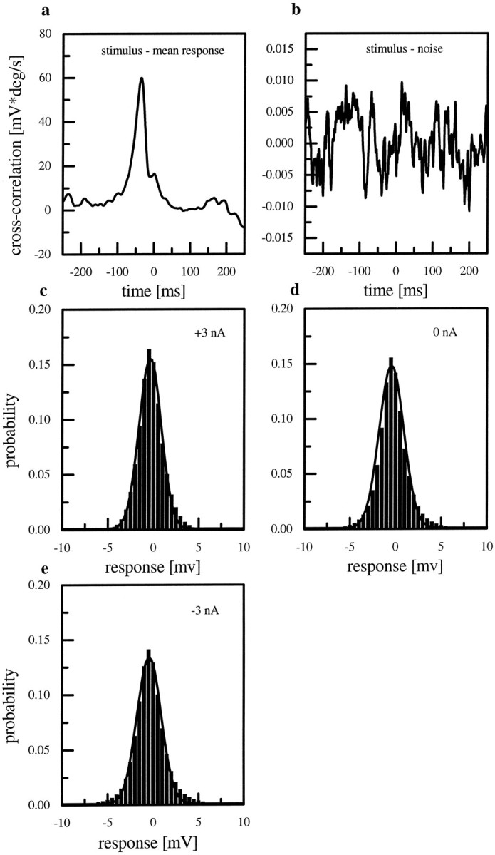
Cross-correlation between stimulus and mean response (a) and between stimulus and noise (b). The values of both curves differ by three orders of magnitude, indicating that the noise is uncorrelated with the stimulus.c–e, Probability distribution of the noise for the three current injections. The solid line shows a Gaussian fit. The distribution does not change if current is injected.

Fig. 8.

a, Expected coherence functions as determined from the signal and noise spectra shown in Figure 6. Because of the highest signal-to-noise ratio for HS-cells at rest the expected coherence was highest too, for this experimental condition.b, Nonlinearity as defined by the difference between the expected and the measured coherence. This nonlinearity is highest when the cells were permanently hyperpolarized, producing full-blown action potentials in response to visual stimulation. The error bars at 1.5 Hz show the SEM for a single representative frequency.

Fig. 9.

a, Mean expected coherence level and SEM between 0.2 and 10 Hz for the three states of the cell (same data as Fig. 8a). The coherence was highest for HS-cells at rest (averaged over n = 16 cells) and reached values of 0.91. The value for depolarized (n = 7) and hyperpolarized cells (n = 11) were approximately 10% lower. b, Mean nonlinearity level and SEM between 0.2 and 10 Hz for the three states of the cell (same data as Fig. 8b). The value for hyperpolarized cells (n = 11) was highest, whereas the values for depolarized (n = 7) and cells at rest (n = 16 cells) are almost identical. (Note different scaling of a and b.)

Fig. 10.

Upper and lower bounds of information rates for the three states of the cell. The error bars show the SEM.

To disentangle the information carried by the graded membrane potential from the information carried by the action potentials that occur in HS-cells when hyperpolarized, we artificially transformed the analog membrane signal of HS-cells (Fig.11b) into a spike train (Fig. 11c) or a response trace without spikes (Fig.11a) by applying a threshold operation. Whenever the membrane potential was above this threshold, the spike was cut out (Fig. 11a) or a unitary pulse of 1 msec duration and 100 mV amplitude was added to the output, which was zero otherwise (Fig.11c). The latter procedure turned the original analog record of the membrane potential into a binary all-or-nothing signal, the same way the action potentials of spiking neurons like the H1-cell are usually recorded extracellularly. The filters (data not shown) and the coherence for the measured membrane potential and the “spike-less” potential trace turned out to be identical (Fig.12). Thus, it seems that the occurrence of spikes is not responsible for the lower coherence of hyperpolarized cells compared with cells at rest.

Fig. 11.

Transformation of the graded membrane potential of a hyperpolarized (−3 nA) HS-cell (b) into a response trace without spikes (a) and a train of action potentials with unitary amplitude and 1 msec duration (c).

Fig. 12.

Comparison of the coherence functions calculated for the measured membrane potential of a hyperpolarized HS-cell (thick line) and the artificially reduced response trace (thin line).

To measure how well the information about the stimulus velocity was retained in this artificial spike train, we applied the same technique as for the analog response traces. Figure13a shows the coherence between stimulus velocity and the analog membrane potential for the hyperpolarized cell (thin line) and the coherence between stimulus velocity and the spike train (thick line). In general, the coherence between the stimulus velocity and the membrane potential was significantly higher than the coherence between stimulus velocity and the spike train. An examination of the difference between measured and expected coherence as a measure of nonlinearity in the signals revealed that the diminished coherence was only partly attributable to different degrees of nonlinearity (Fig. 13b). In fact, the degree of nonlinearity was rather similar under both conditions (note different scales on the y -axes of Fig. 13a,b). Thus, the difference between the measured coherences of graded response versus spike train was largely attributable to a decreased signal-to-noise ratio after the graded response was thresholded.

Fig. 13.

a, Coherence functions calculated for the membrane potential of hyperpolarized HS-cells (thin line; n = 6 cells) and spike trains (thick line; n = 6 cells). The root mean square error for the membrane potential was 86.2 ± 1.1°/sec and 91.5 ± 1.2°/sec for the spike train. The coherence calculated from the membrane potential was much higher than the one from the spike train.b, Nonlinearity, i.e., difference between the expected and the measured coherence for the membrane potential and the spike train. The error bars at 1.5 Hz show the SEM for a single representative frequency.

In Figure 11b, the spikes of HS-cells can be seen to have variable amplitudes. To test whether the amplitude of the spikes carries some information, we again transformed the analog membrane potential of hyperpolarized HS-cells into spike trains with unitary duration. In contrast to Figure 11c, the amplitude of the spikes was not set to a unitary value but left the same as the amplitude of the original spike. This transformation did not result in a greater coherence compared with the spike train with unitary amplitude (data not shown).

Because our previous study (Haag and Borst, 1997) revealed that the spiking H1-cell exhibited a lower coherence than the graded HS-cell, the outcome of the comparison between the graded and the thresholded HS-cell response was not surprising: spikes were elicited only in response to motion in the preferred direction, whereas the graded membrane response could be shifted in both directions. Because of the low spontaneous frequency, there was very little information in the spike train about motion in the anti-preferred direction. This limitation of spike trains applied to the spiking H1-cell as well as the artificially spiking HS-cell. We therefore compared the spikes obtained by thresholding the response of HS-cells with the spikes as recorded from the H1-cell. We found that the spiking HS-cell showed a lower coherence than the H1-cell (Fig.14a). The main deviation of the coherences for both cell types was between 1 and 20 Hz. In that range the measured coherence for the HS-cell was ∼20% lower than the coherence found for the H1-cell. For HS-cells the signal as well as the noise was much lower than the respective values for the H1-neuron (Fig.14b). This was attributable to the low average firing rate found for the HS-cells. H1-cells responded with an average firing rate of 48 ± 1 spikes/sec during the stimulation. HS-cells fired with an average rate of 11 ± 0.5 spikes/sec in response to the identical stimulus.

Fig. 14.

a, Comparison between the coherence functions calculated from the spike trains of HS-cells (thick line; n = 6 cells) and H1-cells (thin line; n = 10 cells). b, Signal and noise spectra for HS- and H1-cells. The amplitude of the signal and the noise of HS-cells is much lower compared with H1-cells. c,Signal-to-noise ratio derived from the data shown in b. d,Nonlinearity in the responses of HS- and H1-cells.

When we calculated signal-to-noise ratios, we found that these ratios were also smaller in HS-cells than in H1-cells (Fig. 14c). In contrast, the degree of nonlinearity, i.e., the difference between measured and expected coherence, was about the same for both cell types (Fig. 14d). From these SNRs, we again calculated channel capacities for the HS spike traces and H1-cells. The information rate for HS-cells (upper bound, 67 bits/sec; lower bound, 13 bits/sec) was lower than for H1-cells (upper bound, 79 bits/sec; lower bound, 23 bits/sec) in the frequency range of 0.25–50 Hz. We also calculated the amount of information carried by a single action potential simply by dividing the upper and the lower bound information rate in bits per second by the number of spikes counted per second. This procedure resulted in a high information content of approximately 6 bits (upper bound) and 1.2 bits (lower bound) per spike of the HS-cells as compared with only 1.7 bits (upper bound) and 0.5 bits (lower bound) per spike for the H1-cells. Because the original information rates of both cells were rather similar, the large difference in the information per action potential was attributable to the low average firing rate found in HS-cells as compared with H1-cells. To examine the influence of a low spike rate on the information content, we artificially decreased the average spike frequency of H1-cells by taking only every fourth spike of the original record of the motion response into consideration. This reduction of the number of spikes led to an average rate of 12 spikes/sec, which is comparable to the response of HS-cells. The coherence for this artificially reduced spike train of H1-cells together with the coherence for spike trains from H1- and HS-cells is shown in Figure 15a. The reduction of the number of spikes mainly led to a decreased coherence for frequencies between 3 and 30 Hz. The coherence for these higher frequencies became as low as the coherence of HS-cells (Fig.15c). Thus, 75% of all the H1 spikes are responsible for the small improvement of ∼20% coherence in this frequency range.

Fig. 15.

a, Comparison between the coherence functions for spike trains of H1- and HS-cells. The reduction of the number of H1-spikes by 75% (dotted line; n= 10 cells) led to a decreased coherence mainly for frequencies >3 Hz. It became as low as the coherence of HS-cells (thick line;n = 6 cells) in this frequency range. b,Mean coherence level and SEM for H1-, reduced spikes of H1-, and HS-cells between 0.2 and 3 Hz. c, Mean coherence level and SEM between 3 and 30 Hz.

DISCUSSION

In this paper, we investigated the influence of active membrane properties on the encoding of stimulus velocity in the neural signals of a motion-sensitive interneuron of the fly visual system, the HS-cell. These cells are characterized by a low resting potential (approximately −50 mV) and a graded potential shift with spike-like events superimposed in response to visual motion stimuli. The injection of depolarizing current while the visual response of the cell was measured led to a reduction in the number and amplitude of these action potentials. The injection of hyperpolarizing current induced full-blown action potentials in response to excitatory visual stimuli. This allowed us to study the same cell type in different response regimes.

In this context it is important to ask to what extent the recorded response properties and resting potentials of HS-cells reflect the properties of the cell without electrode impalement. Of course, absolute certainty about this point is impossible, but on the basis of the following results we are confident that the response properties are not artificial. (1) Intracellular recordings with the same type of electrodes from other motion-sensitive interneurons (e.g., H1-cells) that possess much thinner axons than HS-cells resulted in reliable resting potentials of approximately −60 mV. Under these conditions, H1-cells were found to always produce large-amplitude action potentials (Haag, 1994). (2) Although the action potentials of the spiking H1-cell can be easily recorded with an extracellular electrode, no such recordings have ever been reported from HS-cells. (3) The impalement of the dendrite or the axon of HS-cells by a second intracellular electrode has no influence on response properties and resting potential (Haag and Borst, 1996) or the input resistance (J. Haag and A. Borst, unpublished observations) of the cell.

To evaluate the coding quality of the neural signals under the different conditions caused by the current injection, we calculated the coherence between the stimulus and responses. This value is confined between 0 and 1 and is also known as the correlation coefficient in case of scalar value pairs. It measures the amount of scatter of the data points around the linear regression line. Clearly, a large scatter and thus a low coherence can have two causes: (1) there is a large amount of noise present in the transformation between stimulus and response, or (2) the transformation from the stimulus to the response is nonlinear by nature or both. We disentangled these two sources for a reduced coherence by measuring, in addition to the coherence, the signal-to-noise ratio in the responses by repeated stimulus presentations. Assuming a purely linear stimulus–response relationship, we calculated an expected coherence based on these measured signal-to-noise ratios. The difference between a value of 1 and the expected coherence thus could be attributed to noise, whereas the remaining difference between the expected and the measured coherence had to be caused by nonlinear encoding.

We found that HS-cells without an electrical manipulation represented motion information with a higher precision than electrically manipulated cells. Depolarization as well as hyperpolarization of the cells led to a decrease in coherence. In the depolarizing cells, this decrease was exclusively attributable to a lower signal-to-noise ratio of the motion responses. Compared with the cells at rest, the noise level did not change, whereas the amplitude of the mean response decreased. This was most likely caused by an inactivation of voltage-dependent channels that normally amplify the motion response of the cells at rest. Because the noise level was the same for the depolarized cell and the cell at rest, we conclude that active membrane processes do not contribute much to the noise level of these cells at resting potential. In the hyperpolarized cells the decrease of the coherence was again attributable to a lower SNR, but in addition to an increased nonlinearity in the response. The lower SNR resulted from an increased noise level. Thus, the larger contribution of voltage-dependent processes did not further amplify the mean response but did enhance the amplitude of the noise. In addition, the response also became more nonlinear under these conditions. It appears that the resting potential of the cells represents an ideal set-point where image velocity can be optimally represented by the membrane potential of the cell. Thus, in contrast to our expectation, active processes, when tuned in just the right way, do not deteriorate the representation of image velocity in the neural signal of HS-cells by the introduction of nonlinearities or an increase of noise but rather enhance the coding efficiency by amplifying signals but not noise. This could be accomplished, e.g., by a regional differentiation between signal and noise going along with a spatially inhomogeneous distribution of amplification mechanisms. Whether the dominant noise source is intrinsic to HS-cells or caused by presynaptic circuitry remains to be clarified. In any case, it will be important to gain a detailed understanding at the biophysical level of the intricate interplay between the intrinsic active membrane properties of HS-cells and their synaptic input signals and the consequences for their coding capabilities. Biophysically realistic compartmental models of HS-cells, which were developed recently in our laboratory (Borst and Haag, 1996;Haag et al., 1997), shall prove a useful tool in this context.

As a consequence of the maximum SNR of HS-cells at rest, the channel capacity was also maximum under these conditions. The same was true for the lower bound on the information rate. When calculating lower and upper bounds, we restricted the frequency range to an upper limit of 50 Hz, because given a frame rate of 200 Hz of our stimulus device the highest velocity modulation that we could produce amounted to 50 Hz. We found a channel capacity at rest of 110 bits/sec. This information rate is rather low compared with the large monopolar cells of the fly visual system, which are postsynaptic to the photoreceptors and exhibit, depending on the mean light level, a temporal low-pass or bandpass filter characteristic (van Hateren 1992a,b). Large monopolar cells respond to changes in light intensity by a graded shift of membrane potential as HS-cells do. The upper limit of the rate at which these cells transmit information about the light intensity was measured to 1650 bits/sec (de Ruyter van Steveninck and Laughlin, 1996) and thus is ∼15 times higher than the maximum possible rate at which HS-cells could transmit information about the stimulus velocity. This huge difference probably reflects the fact that in the case of the large monopolar cells the light intensity is already represented at the photoreceptor output synapse, whereas the velocity signal is not a stimulus parameter uniquely encoded by the synaptic input but rather is being calculated, at least in part, on the dendrite of the LPTCs (Single et al., 1997).

The comparison between the membrane potential and the artificially produced spike trains obtained by thresholding the visual responses of hyperpolarized HS-cells revealed that the analog membrane potential carried more information than the binary all-or-nothing spike train. This is most likely attributable to the fact that when the average spontaneous firing rate is low, spikes can transmit information almost exclusively about one direction of the motion stimulus, whereas graded responses can follow both directions of the motion stimuli without any immediate ceiling effects (Haag and Borst, 1997). The comparison of the spike trains of H1- and HS-cells showed that more information about the stimulus was retained in the spike train of H1-cells. This is most likely because of the lower spike frequency of HS-cells.

Another question arising from this work concerns the way information is transmitted from HS-cells to postsynaptic cells. If there is a graded transmitter release (e.g., Angstadt and Calabrese, 1991; Laurent, 1993) without any threshold, the information contained in the graded membrane response of HS-cells can be fully transmitted to the next cell. A threshold operation would introduce further nonlinearities in the response of the postsynaptic cell to visual motion stimuli. More importantly, information about the null direction motion that is inherent only in the graded membrane response of HS-cells but not in its spike-like depolarization could not be transmitted through this synapse. This seems to be unlikely, because HS-cells are the only known horizontal-sensitive large-field output elements of the lobula plate (Hausen, 1984), and thus flies could not respond to null-direction motion. However, motion stimuli going from back to front and thus along the null direction of the HS-cells have been found to elicit significant optomotor responses in flies (Wehrhahn, 1981; Borst et al., 1991). The information theoretical analysis of postsynaptic cells will show how much of the information about null-direction motion that is inherent in the analog membrane potential of HS-cells is indeed transmitted to these postsynaptic neurons.

REFERENCES

- 1.Angstadt JD, Calabrese RL. Calcium currents and graded synaptic transmission between heart interneurons of the leech. J Neurosci. 1991;11:746–759. doi: 10.1523/JNEUROSCI.11-03-00746.1991. [DOI] [PMC free article] [PubMed] [Google Scholar]
- 2.Bialek W, Rieke F. Reliability and information transmission in spiking neurons. Trends Neurosci. 1992;15:428–434. doi: 10.1016/0166-2236(92)90005-s. [DOI] [PubMed] [Google Scholar]
- 3.Bialek W, Rieke F, de Ruyter van Steveninck R, Warland D. Reading a neural code. Science. 1991;252:1854–1857. doi: 10.1126/science.2063199. [DOI] [PubMed] [Google Scholar]
- 4.Borst A, Egelhaaf M. Principles of visual motion detection. Trends Neurosci. 1989;12:297–306. doi: 10.1016/0166-2236(89)90010-6. [DOI] [PubMed] [Google Scholar]
- 5.Borst A, Egelhaaf M. Direction selectivity of fly motion-sensitive neurons is computed in a two-stage process. Proc Natl Acad Sci USA. 1990;87:9363–9367. doi: 10.1073/pnas.87.23.9363. [DOI] [PMC free article] [PubMed] [Google Scholar]
- 6.Borst A, Haag J. The intrinsic electrophysiological characteristics of fly lobula plate tangential cells. I. Passive membrane properties. J Comput Neurosci. 1996;3:313–336. doi: 10.1007/BF00161091. [DOI] [PubMed] [Google Scholar]
- 7.Borst A, Buchstäber F, Egelhaaf M. Synapse—Transmission—Modulation (Elsner N, Penzlin H, eds, p. 262. Thieme; Stuttgart: 1991. Spatial integration of visual motion information in the optomotor response of the housefly. [Google Scholar]
- 8.Bullock TH. Spikeless neurones: where do we go from here? In: Roberts A, Bush BMH, editors. Neurones without impulses. Cambridge UP; Cambridge, UK: 1981. pp. 269–284. [Google Scholar]
- 9.Callaway JC, Ross WN. Frequency-dependent propagation of sodium action potentials in dendrites of hippocampal CA1 pyramidal neurons. J Neurophysiol. 1995;74:1395–1403. doi: 10.1152/jn.1995.74.4.1395. [DOI] [PubMed] [Google Scholar]
- 10.Cover TM, Thomas JA. Elements of information theory. Wiley; New York: 1991. [Google Scholar]
- 11.de Ruyter van Steveninck RR, Laughlin SB. The rate of information transfer at graded-potential synapses. Nature. 1996;379:642–645. [Google Scholar]
- 12.Egelhaaf M, Borst A, Reichardt W. Computational structure of a biological motion detection-detection system as revealed by local detector analysis in the fly’s nervous system. J Opt Soc Am A. 1989;6:1070–1087. doi: 10.1364/josaa.6.001070. [DOI] [PubMed] [Google Scholar]
- 13.Gabbiani F, Metzner W, Wessel R, Koch C. From stimulus encoding to feature extraction in weakly electric fish. Nature. 1996;384:564–567. doi: 10.1038/384564a0. [DOI] [PubMed] [Google Scholar]
- 14.Haag J (1994) Aktive und passive Membraneigenschaften bewegungsempfindlicher Interneurone der Schmeißfliege Calliphora erythrocephala. PhD thesis, Tuebingen.
- 15.Haag J, Borst A. Amplification of high-frequency synaptic inputs by active dendritic membrane processes. Nature. 1996;379:639–641. [Google Scholar]
- 16.Haag J, Borst A. Encoding of visual motion information and reliability in spiking and graded potential neurons. J Neurosci. 1997;17:4809–4819. doi: 10.1523/JNEUROSCI.17-12-04809.1997. [DOI] [PMC free article] [PubMed] [Google Scholar]
- 17.Haag J, Theunissen F, Borst A. The intrinsic electrophysiological characteristics of fly lobula plate tangential cells. II. Active membrane properties. J Comput Neurosci. 1997;4:349–369. doi: 10.1023/a:1008804117334. [DOI] [PubMed] [Google Scholar]
- 18.Hausen K. Motion sensitive interneurons in the optomotor system of the fly. I. The horizontal cells: structure and signals. Biol Cybern. 1982a;45:143–156. [Google Scholar]
- 19.Hausen K. Motion sensitive interneurons in the optomotor system of the fly. II. The horizontal cells: receptive field organization and response characteristics. Biol Cybern. 1982b;46:67–79. [Google Scholar]
- 20.Hausen K. The lobula-complex of the fly: structure, function and significance in visual behaviour. In: Ali MA, editor. Photoreception and vision in invertebrates. Plenum; New York: 1984. pp. 523–559. [Google Scholar]
- 21.Hengstenberg R. Spike response of “non-spiking” visual interneurone. Nature. 1977;270:338–340. doi: 10.1038/270338a0. [DOI] [PubMed] [Google Scholar]
- 22.Hirsch JA, Gilbert CD. Synaptic physiology of horizontal connections in the cat’s visual cortex. J Neurosci. 1991;11:1800–1809. doi: 10.1523/JNEUROSCI.11-06-01800.1991. [DOI] [PMC free article] [PubMed] [Google Scholar]
- 23.Laurent G. A dendritic gain control mechanism in axonless neurons of the locust, Schistocerca Americana. J Physiol (Lond) 1993;470:45–54. doi: 10.1113/jphysiol.1993.sp019846. [DOI] [PMC free article] [PubMed] [Google Scholar]
- 24.Press WH, Flannery BP, Teukolsky SA, Vetterling WT. Numerical recipes in C. The art of scientific computing. Cambridge, UP; Cambridge, UK: 1988. [Google Scholar]
- 25.Shannon CE, Weaver W. The mathematical theory of communication. The University of Illinois; Chicago: 1949. [Google Scholar]
- 26.Rieke F, Warland D, de Ruyter van Steveninck R, Bialek W. Spikes: exploring the neural code. MIT; Cambridge, MA: 1997. [Google Scholar]
- 27.Single S, Haag J, Borst A. Dendritic computation of direction selectivity and gain control in visual interneurons. J Neurosci. 1997;17:6023–6030. doi: 10.1523/JNEUROSCI.17-16-06023.1997. [DOI] [PMC free article] [PubMed] [Google Scholar]
- 28.Spruston N, Schiller Y, Stuart G, Sakmann B. Activity-dependent action potential invasion and calcium influx into hippocampal CA1 dendrites. Science. 1995;268:297–300. doi: 10.1126/science.7716524. [DOI] [PubMed] [Google Scholar]
- 29.Stuart GJ, Sakmann B. Active propagation of somatic action potentials into neocortical pyramidal cell dendrites. Nature. 1994;367:69–72. doi: 10.1038/367069a0. [DOI] [PubMed] [Google Scholar]
- 30.Theunissen F (1993) An investigation of sensory coding principles using advanced statistical techniques. PhD dissertation, University of California at Berkeley.
- 31.Theunissen F, Roddey JC, Stufflebeam S, Clague H, Miller JP. Information theoretic analysis of dynamical encoding by four primary sensory interneurons in the cricket cercal system. J Neurophysiol. 1996;75:1345–1364. doi: 10.1152/jn.1996.75.4.1345. [DOI] [PubMed] [Google Scholar]
- 32.van Hateren JH. Theoretical predictions of spatiotemporal receptive fields of fly LMCs, and experimental validation. J Comp Physiol [A] 1992a;171:157–170. [Google Scholar]
- 33.van Hateren JH. Real and optimal neural images in early vision. Nature. 1992b;360:68–70. doi: 10.1038/360068a0. [DOI] [PubMed] [Google Scholar]
- 34.Wehrhahn C. Fast and slow flight torque responses in flies and their possible role in visual orientation. Biol Cybern. 1981;40:213–221. [Google Scholar]
- 35.Yuste R, Tank DW. Dendritic integration in mammalian neurons, a century after Cajal. Neuron. 1996;16:701–716. doi: 10.1016/s0896-6273(00)80091-4. [DOI] [PubMed] [Google Scholar]
- 36.Yuste R, Gutnick MJ, Saar D, Delaney KR, Tank DW. Ca2+ accumulations in dendrites of neocortical pyramidal neurons: an apical band and evidence for two functional compartments. Neuron. 1994;13:23–43. doi: 10.1016/0896-6273(94)90457-x. [DOI] [PubMed] [Google Scholar]