A Statistical Paradigm for Neural Spike Train Decoding Applied to Position Prediction from Ensemble Firing Patterns of Rat Hippocampal Place Cells

Abstract

The problem of predicting the position of a freely foraging rat based on the ensemble firing patterns of place cells recorded from the CA1 region of its hippocampus is used to develop a two-stage statistical paradigm for neural spike train decoding. In the first, or encoding stage, place cell spiking activity is modeled as an inhomogeneous Poisson process whose instantaneous rate is a function of the animal’s position in space and phase of its theta rhythm. The animal’s path is modeled as a Gaussian random walk. In the second, or decoding stage, a Bayesian statistical paradigm is used to derive a nonlinear recursive causal filter algorithm for predicting the position of the animal from the place cell ensemble firing patterns. The algebra of the decoding algorithm defines an explicit map of the discrete spike trains into the position prediction. The confidence regions for the position predictions quantify spike train information in terms of the most probable locations of the animal given the ensemble firing pattern. Under our inhomogeneous Poisson model position was a three to five times stronger modulator of the place cell spiking activity than theta phase in an open circular environment. For animal 1 (2) the median decoding error based on 34 (33) place cells recorded during 10 min of foraging was 8.0 (7.7) cm. Our statistical paradigm provides a reliable approach for quantifying the spatial information in the ensemble place cell firing patterns and defines a generally applicable framework for studying information encoding in neural systems.

Neural systems encode their representations of biological signals in the firing patterns of neuron populations. Mathematical algorithms designed to decode these firing patterns offer one approach to deciphering how neural systems represent and transmit information. To illustrate, the spiking activity of CA1 place cells in the rat hippocampus correlates with both the rat’s position in its environment and the phase of the theta rhythm as the animal performs spatial behavioral tasks (O’Keefe and Dostrovsky, 1971; O’Keefe and Reece, 1993; Skaggs et al., 1996). Wilson and McNaughton (1993) used occupancy-normalized histograms to represent place cell firing propensity as a function of a rat’s position in its environment and a maximum correlation algorithm to decode the animal’s position from the firing patterns of the place cell ensemble. Related work on population-averaging and tuning curve methods has been reported by Georgopoulos et al. (1986), Seung and Sompolinsky (1993), Abbott (1994), Salinas and Abbott (1994), and Snippe (1996).

Spike train decoding has also been studied in a two-stage approach using Bayesian statistical methods (Bialek and Zee, 1990; Bialek et al., 1991; Warland et al., 1992; Sanger 1996; Rieke et al., 1997; Zhang et al., 1998). The first, or encoding stage, characterizes the probability of neural spiking activity given the biological signal, whereas the second, or decoding stage, uses Bayes’ rule to determine the most probable value of the signal given the spiking activity. The Bayesian approach is a general analytic framework that, unlike either the maximum correlation or population-averaging methods, has an associated paradigm for statistical inference (Mendel, 1995). To date four practices common to the application of the Bayesian paradigm in statistical signal processing have yet to be fully applied in decoding analyses. These are (1) using a parametric statistical model to represent the dependence of the spiking activity on the biological signal and to test specific biological hypotheses; (2) deriving formulae that define the explicit map of the discrete spike trains into the continuous signal predictions; (3) specifying confidence regions for the signal predictions derived from ensemble spike train activity; and (4) implementing the decoding algorithm recursively. Application of these practices should yield better quantitative descriptions of how neuron populations encode information.

For example, the estimated parameters from a statistical model would provide succinct, interpretable representations of salient spike train properties. As a consequence, statistical hypothesis tests can be used to quantify the relative biological importance of model components and to identify through goodness-of-fit analyses spike train properties the model failed to describe. A formula describing the mapping of spike trains into the signal would demonstrate exactly how the decoding algorithm interprets and converts spike train information into signal predictions. Confidence statements provide a statistical measure of spike train information in terms of the uncertainty in the algorithm’s prediction of the signal. Under a recursive formulation, decoding would be conducted in a causal manner consistent with the sequential way neural systems update; the current signal prediction is computed from the previous signal prediction plus the new information in the spike train about the change in the signal since the previous prediction.

We use the problem of position prediction from the ensemble firing patterns of hippocampal CA1 place cells recorded from freely foraging rats to develop a comprehensive, two-stage statistical paradigm for neural spike train decoding that applies the four signal processing practices stated above. In the encoding stage we model place cell spiking activity as an inhomogeneous Poisson process whose instantaneous firing rate is a function of the animal’s position in the environment and phase of the theta rhythm. We model the animal’s path during foraging as a Gaussian random walk. In the decoding stage we use Bayesian statistical theory to derive a nonlinear, recursive causal filter algorithm for predicting the animal’s position from place cell ensemble firing patterns. We apply the paradigm to place cell, theta phase, and position data from two rats freely foraging in an open environment.

MATERIALS AND METHODS

Experimental methods

Two approximately 8-month-old Long–Evans rats (Charles River Laboratories, Wilmington, MA) were implanted with microdrive arrays housing 12 tetrodes (four wire electrodes) (Wilson and McNaughton, 1993) using surgical procedures in accordance with National Institutes of Health and Massachusetts Institute of Technology guidelines. Anesthesia was induced with ketamine 50 mg/kg, xylazine 6 mg/kg, and ethanol 0.35 cc/kg in 0.6 cc/kg normal saline and maintained with 1–2% isoflurane delivered by mask. The skin was incised, the skull was exposed, and six screw holes were drilled. The skull screws were inserted to provide an anchor for the microdrive assembly. An additional hole was drilled over the right CA1 region of the hippocampus (coordinates, −3.5 anteroposterior, 2.75 lateral). The dura was removed, the drive was positioned immediately above the brain surface, the remaining space in the hole was filled with bone wax, and dental acrylic was applied to secure the microdrive assembly holding the tetrodes to the skull. Approximately 2 hr after recovery from anesthesia and surgery, the tetrodes were advanced into the brain. Each tetrode had a total diameter of ∼45 μm, and the spacing between tetrodes was 250–300 μm. The tips of the tetrodes were cut to a blunt end and plated with gold to a final impedance of 200–300 KΩ.

Over 7 d, the electrodes were slowly advanced to the pyramidal cell layer of the hippocampal CA1 region. During this period the animals were food-deprived to 85% of their free-feeding weight and trained to forage for randomly scattered chocolate pellets in a black cylindrical environment 70 cm in diameter with 30-cm-high walls (Muller et al., 1987). Two cue cards, each with different black-and-white patterns, were placed on opposite sides of the apparatus to give the animals stable visual cues. Training involved exposing the animal to the apparatus and allowing it to become comfortable and explore freely. After a few days, the animals began to forage for chocolate and soon moved continuously through the environment.

Once the electrodes were within the cell layer, recordings of the animal’s position, spike activity, and EEG were made during a 25 min foraging period for animal 1 and a 23 min period for animal 2. Position data were recorded by a tracking system that sampled the position of a pair of infrared diode arrays on each animal’s head. The arrays were mounted on a boom attached to the animal’s head stage so that from the camera’s point of view, the front diode array was slightly in front of the animal’s nose and the rear array was above the animal’s neck. Position data were sampled at 60 Hz with each diode array powered on alternate camera frames; i.e., each diode was on for 30 frames/sec, and only one diode was illuminated per frame. The camera sampled a 256 × 364 pixel grid, which corresponded to a rectangular view of 153.6 × 218.4 cm. The animal’s position was computed as the mean location of the two diode arrays in two adjacent camera frames. To remove obvious motion artifact, the raw position data were smoothed off-line with a span 30 point (1 sec) running average filter. Missing position samples that occurred when one of the diode arrays was blocked were filled in by linear interpolation from neighboring data in the off-line analysis.

Signals from each electrode were bandpass-filtered between 600 Hz and 6 kHz. Spike waveforms were amplified 10,000 times and sampled at 31.25 kHz/channel and saved to disk. A recording session consisted of the foraging period bracketed by 30–40 min during which baseline spike activity was recorded while the animal rested quietly. At the completion of the recording session, the data were transferred to a workstation where information about peak amplitudes and widths of the spike waveforms on each of the four channels of the tetrode was used to cluster the data into individual units, and assign each spike to a single cell. For animal 1 (2), 33 (34) place cells were recorded during its 25 (23) min foraging period and used in the place field encoding and decoding analysis.

Continuous EEG data were taken from the same electrodes used for unit recording. One wire from each tetrode was selected for EEG recordings, and the signal was filtered between 1 Hz and 3 kHz, sampled at 2 kHz/channel and saved to disk. The single EEG channel showing the most robust theta rhythm was identified and resampled at 250 Hz, and the theta rhythm was extracted by applying a Fourier filter with a pass band of 6–14 Hz. The phase of the theta rhythm was determined by identifying successive peaks in the theta rhythm and assuming that successive peaks represented a complete theta cycle from 0 and 2π. Each point between the peaks was assigned a phase between 0 and 2π proportional to the fraction of the distance the point lay between the two peaks (Skaggs et al., 1996). The theta rhythm does not have the same phase at different sites of the hippocampus; however, the phase difference between sites is constant. Hence, it is sufficient to model theta phase modulation of place cell spiking activity with the EEG signal recorded from a single site (Skaggs et al., 1996).

Statistical methods

The hippocampus encodes information about the position of the animal in its environment in the firing patterns of its place cells. We develop a statistical model to estimate the encoding process and a statistical algorithm to decode the position of the animal in its environment using our model estimate of the encoding process. We divide the experiment in two parts and conduct the statistical paradigm in two stages: the encoding and decoding stages. We define the encoding stage as the first 15 and 13 min of spike train, path, and theta rhythm data for animals 1 and 2, respectively, and estimate the parameters of the inhomogeneous Poisson process model for each place cell and the random walk model for each animal. We define the decoding stage as the last 10 min of the experiment for each animal and use the ensemble spike train firing patterns of the place cells and random walk parameters determined in the encoding stage to predict position.

To begin we define our notation. Let (0, T] denote the foraging interval for a given animal and assume that within this interval the spike times of C place cells are simultaneously recorded. For animals 1 and 2, T = 25 and 23 min respectively. Let t_i^c denote the spike recorded from cell c at time t_i in (0, T], where c = 1, … , C, and C is the total number of place cells. Let x(t) = [x₁(t), x₂(t)]′ be the 2 × 1 vector denoting the animal’s position at time t, and let φ(t) be the phase of the theta rhythm at time t. The notation x(t)′ denotes the transpose of the vector x(t).

Encoding stage: the place cell model. Our statistical model for the place field is defined by representing the spatial and theta phase dependence of the place cell firing propensity as an inhomogeneous Poisson process. An inhomogeneous Poisson process is a Poisson process in which the rate parameter is not constant (homogeneous) but varies as a function of time and/or some other physical quantity such as space (Cressie, 1993). Here, the rate parameter of the inhomogeneous Poisson process is modeled as a function of the animal’s position in the environment and phase of the theta rhythm. The position component for cell c is modeled as a Gaussian function defined as:

$${\lambda }_x^c(t\Vert x(t),{\xi }_x^c)=exp\left\{{\alpha }_c-\frac{1}{2}(x(t)-{\mu }_c{)}^{\prime }{W}_c^{-1}(x(t)-{\mu }_c)\right\},$$ Equation 1

where μ_c = [μ_c,1, μ_c,2]′ is the 2 × 1 vector whose components are the x₁ and x₂ coordinates of the place field center, α_c is the location intensity parameter,

$$W_c=\left[\begin{array}{cc}{\varsigma }_{c,1}^2& 0\\ 0& {\varsigma }_{c2}^2\end{array}\right]$$ Equation 2

is a scale matrix whose scale parameters in the x₁ and x₂ directions are ς_c,1² and ς_c,2², respectively, and ξ_x^c = [α_c, μ_c, W_c]. Our original formulation of the place cell model included non-zero off-diagonal terms of the scale matrix to allow varying spatial orientations of the estimated place fields (Brown et al., 1996, 1997a). Because we found these parameters to be statistically indistinguishable from zero in our previous analyses, we omit them from the current model. The theta phase component of cell c is modeled as a cosine function defined as:

$${\lambda }_{\theta }^c(t\Vert \phi (t),{\xi }_{\theta }^c)=exp\{{\beta }_{c}cos(\phi (t)-{\phi }_c)\},$$ Equation 3

where β_c is a modulation factor, φ_c is the theta phase of maximum instantaneous firing rate for cell c, and ξ_θ^c = [β_c, φ_c]. The instantaneous firing rate function for cell c is the product of the position component in Equation 1 and the theta rhythm component in Equation 3 and is given as:

$${\lambda }^c(t\Vert x(t),\phi (t),{\xi }_x^c)={\lambda }_x^c(t\Vert x(t),{\xi }_x^c){\lambda }_{\theta }^c(t\Vert \phi (t),{\xi }_{\theta }^c),$$ Equation 4

where ξ^c = [ξ_x^c, ξ_θ^c]. The maximum instantaneous firing rate of place cell c is exp {α_c + β_c} and occurs at x(t) = μ_c and φ(t) = φ_c. The instantaneous firing rate model in Equation4 does not consider the modulation of place cell firing propensity attributable to the interaction between position and theta phase known as phase precession (O’Keefe and Reece, 1993). We assume that individual place cells form an ensemble of conditionally independent Poisson processes. That is, the place cells are independent given their model parameters. In principle, it is possible to give a more detailed formulation of ensemble place cell spiking activity that includes possible interdependencies among cells (Ogata, 1981). Such a formulation is not considered here. The inhomogeneous Poisson model defined in Equations 1-4 was fit to the spike train data of each place cell by maximum likelihood (Cressie, 1993). The importance of the theta phase model component was assessed using likelihood ratio tests (Cassella and Berger, 1990) and Akaike’s Information Criterion (AIC) (Box et al., 1994).

After model fitting we evaluated validity of the Poisson assumption in two ways using the fact that a Poisson process defined on an interval is also a Poisson process on any subinterval of the original interval (Cressie, 1993). First, based on the estimated Poisson model parameters, we computed for each place cell the 95% confidence interval for the true number of spikes in the entire experiment, in the encoding stage and in the decoding stage. In each case, we assessed agreement with the Poisson model by determining whether the recorded number of spikes was within the 95% confidence interval estimated from the model.

Second, for each place cell we identified between 10 to 65 subpaths on which the animal traversed the field of that cell for at least 0.5 sec. The region of the place field we sampled was the ellipse located at the place cell center, which contained 67% of the volume of the fitted Gaussian function in Equation 1. This is equivalent to the area within 1 SD of the mean of a one-dimensional Gaussian probability density. The entrance and exit times for the fields were determined using the actual path of the animal. From the estimate of the exact Poisson probability distribution on each subpath we computed the p value to measure how likely the observed number of spikes was under the null hypothesis of a Poisson model. A small p value would suggest that the data are not probable under the Poisson model, whereas a large p value would suggest that the data are probable and, hence, consistent with the model. If the firing pattern along the subpaths truly arose from a Poisson process, then the histogram of p values should be approximately uniform. A separate analysis was performed for subpaths in the encoding and decoding stages of each animal.

Encoding stage: the path model. We assume that the path of the animal during the experiment may be approximated as a zero mean two-dimensional Gaussian random walk. The random walk assumption means that given any two positions on the path, say x(t_k−1) and x(t_k), the path increments, x(t_k) − x(t_k−1), form a sequence of independent, zero mean Gaussian random variables with covariance matrix:

$$W_x({\mathrm{\Delta }}_k)=\left[\begin{array}{cc}{\varsigma }_{x_1}^2& \rho {\varsigma }_{x_1}{\varsigma }_{x_2}\\ \rho {\varsigma }_{x_1}{\varsigma }_{x_2}& {\varsigma }_{x_2}^2\end{array}\right]{\mathrm{\Delta }}_k,$$ Equation 5

where ς_x1², ς_x2² are the variances of x₁ and x₂ components of the increments, respectively, ρ is the correlation coefficient, and Δ_k = t_k − t_k−1. These model parameters were also estimated by maximum likelihood. Following model fitting, we evaluated the validity of the Gaussian random walk assumption by a χ² goodness-of-fit test and by a partial autocorrelation analysis. In the goodness-of-fit analysis, the Gaussian assumption was tested by comparing the joint distribution of the observed path increments with the bivariate Gaussian density defined by the estimated model parameters. The partial autocorrelation function is an accepted method for detecting autoregressive dependence in time series data (Box et al., 1994). Like the autocorrelation function, the partial autocorrelation function measures correlations between time points in a time series. However, unlike the autocorrelation function, the partial autocorrelation function at lag k measures the correlation between points k time units apart, correcting for correlations at lags k − 1 and lower. An autoregressive model of order p will have a nonzero partial autocorrelation function up through lag p and a partial autocorrelation function of zero at lags p + 1 and higher. Therefore, a Gaussian random walk with independent increments should have uncorrelated increments at all lags and, hence, its partial autocorrelation function should be statistically indistinguishable from zero at all lags (Box et al., 1994).

Decoding stage. To develop our decoding algorithm we first explain some additional notation. Define a sequence of times in (t_e, T], t_e ≤ t₀ < t₁ < t₂, … , t_k < t_k+1, … , < t_K ≤ T, where t_e is the end of the encoding stage. The t_k values are an arbitrary time sequence in the decoding stage, which includes the spike times of all the place cells. We define I_c(t_k) as the indicator of a spike at time t_k for cell c. That is, I_c(t_k) is 1 if there is a spike at t_k from cell c and 0 otherwise. Let I(t_k) = [I₁(t_k), … , I_C(t_k)]′ be the vector of indicator variables for the C place cells for time t_k. The objective of the decoding stage is to find for each t_k the best prediction of x(t_k) in terms of a probability density, given C place cells, their place field and theta rhythm parameters, and the firing pattern of the place cell ensemble from t_e up through t_k. Because the t_k values are arbitrary, the prediction of x(t_k) will be defined in continuous time. An approach suggested by signal processing theory for computing the probability density of x(t_k) given the spikes in (t_e, t_k] is to perform the calculations sequentially. Under this approach Bayes’ rule is used to compute recursively the probability density of the current position from the probability densities of the previous position and that of the new spike train data measured since the previous position prediction was made (Mendel, 1995). The recursion relation is defined in terms of two coupled probability densities termed the posterior and one-step prediction probability densities. For our decoding problem these two probability densities are defined as:

Posterior probability density:

$$\text{Pr}(x(t_k)\Vert spikesin\left(t_e,t_k\right])=$$ Equation 6

$$\frac{\text{Pr}(x(t_k)\Vert spikesin\left(t_e,t_{k-1}\right])\times \text{Pr}(spikesat{t}_k\Vert x(t_k),t_{k-1})}{\text{Pr}(spikesat{t}_k\Vert spikesin\left(t_e,t_{k-1}\right])};$$

One-step prediction probability density:

$$\text{Pr}(x(t_k)\Vert spikesin\left(t_e,t_{k-1}\right])$$ Equation 7

$$=\int \text{Pr}(x(t_{k-1})\Vert spikesin\left(t_e,t_{k-1}\right])\times \text{Pr}(x(t_k)\Vert x(t_{k-1}))\text{dx}(t_{k-1}).$$

Before deriving the explicit form of our decoding algorithm, we explain the terms in Equations 6 and 7 and the logic behind them. The first term on the right side of Equation 6, Pr (x(t_k)‖spikes in(t_e, t_k−1]), is the one-step prediction probability density from Equation 7. It defines the predictions of where the animal is likely to be at time t_k given the spike train data up through time t_k−1. Equation 7 shows that the one-step prediction probability density is computed by “averaging over” the animal’s most likely locations at time t_k−1, given the data up to time t_k−1 and the most likely set of moves it will make in t_k−1 to t_k. The animal’s most likely position at time t_k−1, the first term of the integrand in Equation 7, is the posterior probability density at t_k−1. The animal’s most likely set of moves from t_k−1 to t_k, Pr (x(t_k)‖x(t_k−1)), is defined by the random walk probability model in Equation 5 and again below in Equation 8. The formulae are recursive because Equation 7 uses the posterior probability density at time t_k−1to generate the one-step prediction probability density at t_k, which, in turn, allows computation of the new posterior probability at time t_k given in Equation 6. The second term on the right side of Equation 6, Pr(spikes at t_k‖x(t_k), t_k−1), defines the probability of a spike at t_k given the animal’s position at t_k is x(t_k) and that the last observation was at time t_k−1. This term is the joint probability mass function of all the spikes at t_k and is defined by the inhomogeneous Poisson model in Equations 1-4 and below in Equation 9. Pr(spikes att_k‖spikes in (t_e, t_k−1]) is the integral of the numerator on the right side of Equation 6 and defines the normalizing constant, which ensures that the posterior probability density integrates to 1.

Under the assumption that the individual place cells are conditionally independent Poisson processes and that the path of the rat during foraging in an open environment is a Gaussian random walk, Equations 6and 7 yield the following recursive neural spike train decoding algorithm:

State equation:

$$x(t_k)-x(t_{k-1})\sim N(0,W_x({\mathrm{\Delta }}_k));$$ Equation 8

Observation equation:

$$f(\mathbf{I}(t_k)\Vert x(t_k),t_{k-1})$$ Equation 9

$$=\prod _{c=1}^C \{[{\lambda }^c[x(t_k)]{\mathrm{\Lambda }}^c[\theta ({\mathrm{\Delta }}_k)]{\}}^{I_c(t_k)}exp\{-{\lambda }^c[x(t_k)]{\mathrm{\Lambda }}^c[\theta ({\mathrm{\Delta }}_k)]\};$$

One-step prediction equation:

$$\widehat{x}(t_k\Vert t_{k-1})=\widehat{x}(t_{k-1}\Vert t_{k-1});$$ Equation 10

One-step prediction variance:

$$W(t_k\Vert t_{k-1})=W_x({\mathrm{\Delta }}_k)+W(t_{k-1}\Vert t_{k-1});$$ Equation 11

Posterior mode

$$\widehat{x}(t_k\Vert t_k)={\left[W(t_k\Vert t_{k-1}{)}^{-1}+\sum _{c=1}^C A_c[\widehat{x}(t_k\Vert t_k),\theta ({\mathrm{\Delta }}_k)]W_c^{-1}\right]}^{-1}$$ Equation 12

$$\times \left[W(t_k\Vert t_{k-1}{)}^{-1}\widehat{x}(t_k\Vert t_{k-1})+\sum _{c=1}^C A_c[\widehat{x}(t_k\Vert t_k),\theta ({\mathrm{\Delta }}_k)]W_c^{-1} {\mu }_c\right];$$

Posterior variance:

$$W(t_k\Vert t_k)=\left[W(t_k\Vert t_{k-1}{)}^{-1}+\sum _{c=1}^C A_c[\widehat{x}(t_k\Vert t_k),\theta ({\mathrm{\Delta }}_k)]W_c^{-1}\right.$$ Equation 13

$$+\sum _{c=1}^C {\lambda }^c[\widehat{x}(t_k\Vert t_k)]{\mathrm{\Lambda }}^c[\theta ({\mathrm{\Delta }}_k)]W_c^{-1}(\widehat{x}(t_k\Vert t_k)-{\mu }_c)(\widehat{x}(t_k\Vert t_k)-{\mu }_c{)}^{\prime }{W}_c^{-1}{]}^{-1},$$

where the notation ∼N(0, W_x(Δ_k)) denotes the Gaussian probability density with mean 0 and covariance matrix W_x(Δ_k), f(I(t_k)‖x(t_k), t_k−1) is the joint probability mass function of the spikes at time t_k andx̂(t_k‖t_k) denotes the position prediction at time t_k given the spike train up through time t_k. We also define:

$$A_c[x(t_k\Vert t_k),\theta ({\mathrm{\Delta }}_k)]=I_c(t_k)-{\lambda }^c[x(t_k\Vert t_k)]{\mathrm{\Lambda }}^c[\theta ({\mathrm{\Delta }}_k)];$$ Equation 14

$${\mathrm{\Lambda }}^c[\theta ({\mathrm{\Delta }}_k)]=\underset{t_{k-1}}{\overset{t_k}{\int }}exp\{{\beta }_{c}cos(\phi (t)-{\phi }_c)\}\text{dt},$$ Equation 15

where Λ^c[θ(Δ_k)] is the integral of the theta rhythm process (Eq. 3) on the interval (t_k−1, t_k], and λ^c[x(t_k‖t_k)] = λ_x^c[t_k‖x(t_k), ξ_x^c] is given in Equation 1. The predictionx̂(t_k‖t_k) in Equation12 is the mode of the posterior probability density, and therefore, defines the most probable position prediction at t_k given the ensemble firing pattern of the C place cells from t_e up through t_k. We termx̂(t_k‖t_k), the Bayes’ filter prediction and the algorithm in Equations 8-13 the Bayes’ filter algorithm. As stated above, the algorithm defines a recursion that begins with Equation 10. Under the random walk model, given a prediction x(t_k−1‖t_k−1) at t_k−1, the best prediction of position at t_k, i.e., one step ahead, is the prediction at t_k−1. The error in that prediction, given in Equation 11, reflects both the uncertainty in the prediction at t_k−1, defined by W(t_k−1‖t_k−1), and uncertainty of the random walk in (t_k−1, t_k], defined by W_x(Δ_k). Once the spikes at t_k are recorded, the position prediction at t_k is updated to incorporate this new information (Eq. 12). The uncertainty in this posterior prediction is given by Equation 13. The algorithm then returns to Equation 10 to begin the computations for t_k+1. The derivation of the Bayes’ filter algorithm follows the arguments used in themaximum aposteriori estimate derivation of the Kalman filter (Mendel, 1995) and is outlined in . If the posterior probability density of x(t_k) is approximately symmetric, thenx̂(t_k‖t_k) is also both its mean and median. In this case, the Bayes’ filter is an approximately optimal filter in both a mean square and an absolute error sense. Equation 12 is a nonlinear function of x(t_k‖t_k) that is solved iteratively using a Newton’s procedure. The previous position prediction at each step serves as the starting value. Using Equation 13and a Gaussian approximation to the posterior probability density of x(t_k) (Tanner, 1993), an approximate 95% confidence (highest posterior probability density) region for x(t_k) can be defined by the ellipse:

$$[x(t_k)-\widehat{x}(t_k\Vert t_k){]}^{\prime }W(t_k\Vert t_k)[x(t_k)-\widehat{x}(t_k\Vert t_k)]\le 6,$$ Equation 16

where 6 is the 0.95th quantile of the χ²distribution with 2 df.

Interpretation of the Bayes’ filter algorithm. The Bayes’ filter algorithm has a useful analytic interpretation. Equation 12shows explicitly how the discrete spike times, I_c(t_k) values, are mapped into a continuous position predictionx̂(t_k‖t_k). This equation shows that the current position prediction,x̂(t_k‖t_k), is a weighted average of the one-step position prediction,x̂(t_k‖t_k−1), and the place cell centers. The weight on the one-step prediction is the inverse of the one-step prediction covariance matrix (Eq. 11). If the one-step prediction error is high, the one-step prediction receives less weight, whereas if the one-step prediction error is small, the one-step prediction receives more weight. The weight on the one-step prediction also decreases as Δ_k increases (Eq. 11).

The weight on each place cell’s center is determined by the product of a dynamic or data-dependent component attributable to A_c in Equation 14 and a fixed component attributable to the inverse of the scale matrices, the W_c values, in Equation 2. For small Δ_k, it follows from the definition of the instantaneous rate function of a Poisson process that A_c may be reexpressed as:

$$A_c[x(t_k),\theta ({\mathrm{\Delta }}_k)]=I_c(t_k)-{\text{Pr}}^c(spikeat{t}_k\Vert x(t_k),\theta ({\mathrm{\Delta }}_k)).$$ Equation 17

Eq. 17 shows that A_c is equal to either 0 or 1 minus the probability of a spike from cell c at t_k given the position at t_k and the modulation of the theta rhythm in Δ_k. Thus, for small Δ_k, A_c gives a weight in the interval (−1, 1). A large positive weight is obtained if a spike is observed when a place cell has a low probability of a spike at t_k given its geometry and the current phase of the theta rhythm. This is a rare event. A large negative weight is obtained if no spike is observed when a cell has a high probability of firing. This is also a rare event. Equation 12 shows that even when no cell fires the algorithm still provides information about the animal’s most probable position. For example, if no place cell fires at t_k, then all the place cell means receive negative weights, and the algorithm interprets the new information in the firing pattern as suggesting where the animal is not likely to be. The inverse of the scale matrices are the fixed components of the weights on the place cell means and reflect the geometry of the place fields. Place cells whose scale matrices have small scale factors—highly precise fields—will be weighted more in the new position prediction. Conversely, place cells with large scale factors—diffuse place fields—will be weighted less. Viewed as a function of c and t_k, A_c defines for cell c at time t_k the point process equivalent of the innovations in the standard Kalman filter algorithm (Mendel, 1995).

At each step the Bayes’ filter algorithm provides two estimates of position and for each an associated estimate of uncertainty. The one-step position prediction and error estimates are computed before observing the spikes at t_k, whereas the posterior position prediction and error estimates are computed after observing the spikes at t_k. Because the t_k values are arbitrary, the Bayes’ filter provides predictions of the animal’s position in continuous time. The recursive formulation of this algorithm ensures that all spikes in (t_e, t_k] are used to compute the predictionx̂(t_k‖t_k). The Newton’s method of implementation of the algorithm shows the expected quadratic convergence in two to four steps when the previous position is the initial guess for predicting the new position. Because the previous position prediction is a good initial guess, and the distance between the initial guess and the final new position prediction is small, a fast, linear version of Equation 12 can be derived by taking only the first Newton’s step of the procedure. This is equivalent to replacing x̂(t_k‖t_k) on the right side of Equation 12 withx̂(t_k‖t_k−1).

The representation of our decoding algorithm in Equations 8-13 shows the relation of our methods to the well known Kalman filter (Mendel, 1995). Although the equations appear similar to those of the standard Kalman filter, there are important differences. Both the observation and the state equations in the standard Kalman filter are continuous linear functions of the state variable. In the current problem, the state equation is a continuous function of the state variable, the animal’s position. However, the observation process, the neural spike trains, is a multivariate point process and a nonlinear function of the state variable. Our algorithm provides a solution to the problem of estimating a continuous state variable when the observation process is a point process.

Bayes’ smoother algorithm. The acausal decoding algorithms of Bialek and colleagues (1991) are derived in the frequency domain using Wiener kernel methods. These acausal algorithms give an estimate of x(t_k‖T) rather than x(t_k‖t_k) because they use all spikes observed during the decoding stage of the experiment to estimate the signal at each t_k. To compare our algorithm directly with the acausal Wiener kernel methods, we computed the corresponding estimate of x(t_k‖T) in our paradigm. The estimates of x(t_k‖T) and W(t_k‖T) can be computed directly fromx̂(t_k‖t_k),x̂(t_k‖t_k−1), W(t_k‖t_k), and W(t_k‖t_k−1) by the following linear algorithm:

$$A_k=W(t_k\Vert t_k)W(t_{k+1}\Vert t_k{)}^{-1};$$ Equation 18

$$\widehat{x}(t_k\Vert T)=\widehat{x}(t_k\Vert t_k)+A_k[\widehat{x}(t_{k+1}\Vert T)-\widehat{x}(t_{k+1}\Vert t_k)];$$ Equation 19

$$W(t_k\Vert T)=W(t_k\Vert t_k)+A_k[W(t_{k+1}\Vert T)-W(t_{k+1}\Vert t_k)]A_k^{\prime },$$ Equation 20

where the initial conditions are x̂(T‖T) and W(T‖T) obtained from the last step of the Bayes’ filter. Equations 18-20 are the well known fixed- interval smoothing algorithm (Mendel, 1995). To distinguish x̂(t_k‖T) from x̂(t_k‖t_k), we term the former Bayes’ smoother prediction.

Non-Bayes decoding algorithms. Linear and maximum likelihood (ML) decoding algorithms can be derived as special cases of Equation12. These are:

$$\widehat{x}(t_k{)}_L={\left[\sum _{c=1}^C n_c({\mathrm{\Delta }}_k^{*})W_c^{-1}\right]}^{-1} \sum _{c=1}^C n_c({\mathrm{\Delta }}_k^{*})W_c^{-1} {\mu }_c,$$ Equation 21

and

$$\widehat{x}(t_k{)}_{ML}={\left[\sum _{c=1}^C A_c^{*}[\widehat{x}(t_k{)}_{ML}]W_c^{-1}\right]}^{-1} \sum _{c=1}^C A_c^{*}[\widehat{x}(t_k{)}_{ML}]W_c^{-1} {\mu }_c,$$ Equation 22

where Δ^*_k is the 1 sec interval ending at t_k, n_c(Δ^*_k) is the number of spikes from cell c in Δ^*_k, and A^*_c is A_c in Equation 14 with I_c(t_k) replaced by n_c(Δ^*_k). The term A^*_c has approximately the same interpretation as A_c in Equation 14. The derivation of these algorithms is also explained in .

For comparison with the findings of Wilson and McNaughton (1993), we also decoded using their maximum correlation (MC) method. This algorithm is defined as follows. Let λ_ij^cdenote the value of the occupancy- normalized histogram of spikes from cell c on pixel ij. The MC prediction at t_k is the pixel that has the largest correlation with the observed firing pattern of the place cells in Δ^*_k. It is defined as:

$$\widehat{x}(t_k{)}_{MC}=\underset{i,j}{max}\left\{\frac{\sum _{c=1}^C(n_c({\mathrm{\Delta }}_k^{*})-\overline{n({\mathrm{\Delta }}_k^{*})})({\lambda }_{\text{ij}}^c-\overline{{\lambda }_{\text{ij}}})}{{\left[\sum _{c=1}^C(n_c({\mathrm{\Delta }}_k^{*})-\overline{n({\mathrm{\Delta }}_k^{*})}{)}^2\right]}^{1/2}{\left[\sum _{c=1}^C({\lambda }_{\text{ij}}^c-\overline{{\lambda }_{\text{ij}}}{)}^2\right]}^{1/2}}\right\},$$ Equation 23

where λ_ij is the average firing rate over the C cells at pixel location ij, and $\overline{n({\mathrm{\Delta }}_k^{*})}$is the average of the spike counts over the C place cells in Δ^*_k.

Implementation of the decoding algorithms. Position decoding was performed using the Bayes’ filter, ML, linear, MC, and Bayes’ smoother algorithms. Decoding with the Bayes’ filter was performed with and without the theta rhythm component of the model. With the exception of the MC algorithm, position predictions were determined in all decoding analyses at 33 msec intervals, the frame rate of the tracking camera. For the MC algorithm the decoding was performed in 1 sec nonoverlapping intervals. The ML prediction at t_k was computed from the spikes in Δ^*_k, the 1 sec time window ending at t_k. To carry out the ML decoding at the frame rate of the camera and to give a fair comparison with the Bayes’ procedures, this time window was shifted along the spike trains every 33 msec for each ML prediction. Hence, there was a 967 msec overlap in the time window used for adjacent ML predictions. The same 1 sec time window and 33 msec time shift were used to compute the linear decoding predictions. We tested time windows of 0.25, 0.5, and 1 sec and chose the latter because the low spike counts for the place cells gave very unstable position predictions for the shorter time intervals even when the intervals were allowed to overlap. For integration time windows longer than 1 sec, the assumption that the animal remained in the same position for the entire time window was less valid. Zhang et al. (1998) found a 1 sec time window to be optimal for their Bayes’ procedures.

Relationship among the decoding algorithms. The Bayes’ filter and the non-Bayes’ algorithms represent distinct approaches to studying neural computation. Under the Bayes’ filter, an estimate of a behavioral state variable, e.g., position at a given time, is computed from the ensemble firing pattern of the CA1 place cells and stored along with an error estimate. The next estimate is computed using the previous estimate, and the information in the firing patterns about how the state variable has changed since the last estimate was computed. For the non-Bayes’ algorithms the computational logic is different. The position estimate is computed from the place cell firing patterns during a short time window. The time window is then shifted 33 msec and the position representation is recomputed. The Bayes’ filter relies both on prior and new information, whereas the non-Bayes’ algorithms use only current information. Because the Bayes’ filter sequentially updates the position representation, it may provide a more biologically plausible description of how position information is processed in the rat’s brain. On the other hand, the non-Bayes’ algorithms provide a tool for studying the spatial information content of the ensemble firing patterns in short overlapping and nonoverlapping time intervals.

The Bayes’ filter is a nonlinear recursive algorithm that gives the most probable position estimate at t_k given the spike trains from all the place cells and theta rhythm information up to through t_k. The ML algorithm yields the most probable position given only the data in a time window ending at t_k. Because this ML algorithm uses a 1 sec time window, it is not the ML algorithm that would be derived from the Bayes’ filter by assuming an uninformative prior probability density. The latter ML algorithm would have a time window of 33 msec. Given the low firing rates of the place cells, an ML algorithm with a 33 msec integration window would yield position predictions that were significantly more erratic than those obtained with a 1 sec window (see Fig. 4). Theta phase information is also not likely to improve prediction accuracy of the ML algorithm, because the 1 sec integration window averages approximately eight theta cycles. In contrast, the Bayes’ filter has the potential to improve the accuracy of its prediction by taking explicit account of the theta phase information. For the Bayes’ filter with Δ_k = 33 msec and an average theta cycle length of 125 msec, each t_k falls on average in one of four different phases of the theta rhythm.

Fig. 4.

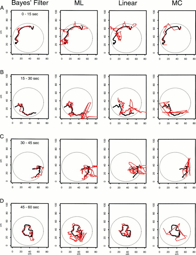
A continuous 60 sec segment of the true path (black line) from animal 2 displayed in four 15 sec intervals along with the predicted paths (red line) from four decoding algorithms. Each column gives the results from the application of one decoding algorithm. The first column is the Bayes’ filter; the second column, the maximum likelihood algorithm (ML); the third column, the linear algorithm; and the fourth column, the maximum correlation procedure (MC). The rows show for each decoding algorithm the true and predicted paths for times 0–15 sec (row A), 15–30 sec (row B), 30–45 sec (row C), and 45–60 sec (row D). For example, third column, row B shows the true path and the linear algorithm prediction for times 15–30 sec. The paths are continuous between the rows within a column; e.g., where the paths end for the Bayes’ filter analysis (first column) at approximately coordinates x₁(t) = 7 cm and x₂(t) = 21 cm in row Ais where they begin in row B. Position predictions are determined at each of the 1800 (60 sec × 30 points/sec) points for each procedure with the exception of the MC algorithm. For the MC algorithm there are 60 predictions computed in nonoverlapping 1 sec intervals. None of the algorithms is constrained to give predictions within the circle. Because of the continuity constraint of the random walk, the Bayes’ filter predictions are less erratic than those of the non-Bayes algorithms.

Equation 16 shows that the local linear decoding algorithm uses no information about previous position or the probability of a place cell firing to determine the position prediction. It simply weights the place cell centers by the product of the number of spikes in the time interval Δ^*_k and the inverse of the scale matrices. If no cell fires, there is no position prediction. Because the algorithm uses no information about the place cell firing propensities, it is expected to perform less well than either the Bayes or the ML algorithms. The MC algorithm estimates the place cell geometries empirically with occupancy-normalized histograms instead of with a parametric statistical model. The position estimate determined by this algorithm is a nonlinear function of the observed firing pattern, and the weighting scheme is determined on a pixel-by-pixel basis by the correlation between the observed firing pattern and the estimated place cell intensities. The MC algorithm is the most computationally intensive of the algorithms studied here because it requires a search at each time step over all pixels in the environment.

The Bayes’ smoother derives directly from the Bayes’ filter by applying the well known fixed-interval smoothing algorithm. Of the five algorithms presented, it uses the most information from the firing pattern to estimate the animal’s position. However, because it uses all future and all past place cell spikes to compute each position estimate, it is the least likely to have a biological interpretation. The Bayes’ smoother is helpful more as an analytic tool than as an actual decoding algorithm because it shows algebraically how current and future information are combined to make its position predictions. This algorithm makes explicit the relation between the Bayes’ filter and a two-sided filter such as the acausal Wiener filter procedures ofBialek et al. (1991).

RESULTS

Encoding stage: evaluation of the Poisson model fit to the place cell firing patterns

The inhomogeneous Poisson model was successfully fit to the place cell spike trains of both animals. Twenty-six of 34 place cells for animal 1 and 24 of 33 cells for animal 2 had place fields located along the border of the environment (Fig. 1). Seven of 34 cells for animal 1 and five of the place cells for animal 2 fired preferentially in regions near the center of the environment. The remaining single cell for animal 1 and four cells for animal 2 had split fields. The split fields could be explained by these place cells having two distinct regions of maximal firing and/or errors in assigning spikes from the tetrode recordings to particular cells. For each of the three types of place field patterns the fits of the position modulation components of the Poisson model were consistent with the occupancy-normalized histograms in terms of shape and location of regions of maximum and minimum firing propensity. For animal 1 (animal 2) 31 (32) of the 34 (33) place cells had statistically significant estimates of the place parameters μ_c,1, μ_c,2, ς_c,1², and ς_c,2², and 27 (33) of the 34 (33) place cells had statistically significant estimates of α.

Fig. 1.

Pseudocolor maps of the fits of the inhomogeneous Poisson model to the place fields of three representative place cells from animal 2. The panels show A, a field lying along the border of the environment; B, a field near the center of the environment; and C, a split field with two distinct regions of maximal firing. Most of the place cells for both animals were like that of cell A (see Encoding stage: evaluation of the Poisson model fit to the place cell firing patterns). The color bars along the right border of each panel show the color map legend in spikes per second. The spike rate near the center of cell A is 25 spikes/sec compared with 12 spikes/sec for cells B and C. Each place field has a nonzero spike rate across a sizable fraction of the circular environment.

In addition to position modulation, there was statistically significant theta phase modulation of the place cell firing patterns for both animals. For animal 1 (2) the theta phases of maximal firing were mostly between 180 and 360° (160 and 360°) with a maximum near 360° (270°). We evaluated the statistical improvement in the fit of the inhomogeneous Poisson model attributable to inclusion of the theta rhythm by likelihood ratio tests and AIC. The likelihood ratio tests showed that 25 of the 34 cells for animal 1 and 31 of the 33 cells for animal 2 had statistically significant improvements in the model fits with the inclusion of the theta component. For 28 of the 34 cells for animal 1 and 31 of the 33 place cells for animal 2, the better model by AIC included the phase of theta rhythm. The individual parameter estimates allow a direct quantitative assessment of the relative importance of position and theta phase on place cell firing. For example, in Fig. 1, place cell B had an estimated maximal firing rate of exp(α + β) = exp(1.91 + 0.56) = 11.82 spikes/sec at coordinates x₁(t) = 40.37, x₂(t) = 43.63, and theta phase φ(t) = 0.61 radians. In the absence of theta phase modulation the approximate maximum firing rate would be exp(α) = exp(1.91) = 6.75 spikes/sec, whereas in the absence of position modulation the maximum firing rate would be exp(β) = exp(0.56) = 1.75 spikes/second. With the exception of five place cells for animal 1 and one cell for animal 2, all the α values were positive and in the range of 0.45–4.5. The β values were all in a narrow range between 0.06 and 0.5 for animal 1 and 0.03 and 1.1 for animal 2. For 25 of 34 place cells for animal 1 and 32 of 33 place cells for animal 2, α was larger than β. The single place cell for animal 2 and the five of seven place cells for animal 1 for which β was larger than α all fired ≤200 spikes during the encoding stage. The median (mean) ratio of exp(α) to exp(β) was 2.9 (5.0) for animal 1 and 5.3 (7.5) for animal 2. Because the median is a more representative measure of central tendency in small groups of numbers (Velleman and Hoaglin, 1981), these findings suggest that position is a three to five times stronger modulator of place cell spiking activity than theta phase under the current model.

Encoding stage: fit of the random walk model to the path

For both animals there was close agreement between the variance components of the Gaussian random walk estimated from the first part of the path (encoding stage) and those estimated from the full path (Eq.5). The estimated variance components were ς_x1 = 0.283 (0.440), ς_x2 = 0.302 (0.393), and ρ = 0.024 (0.033) from the encoding stage for animal 1 (animal 2). The estimated means were all close to zero, and the small values of the correlation coefficient ρ suggested that the x₁ and x₂ components of the random walk are approximately uncorrelated.

Encoding stage: assessment of model assumptions

We present here the results of our goodness-of-fit analyses of the inhomogeneous Poisson model fits to the place cell spike train data and the random walk model fits to the animals’ paths. The implications of these results for our decoding analysis and overall modeling strategy are presented in the Discussion (see Encoding stage: lessons from the random walk and goodness-of-fit analyses).

Evaluation of the inhomogeneous Poisson model goodness-of-fit

In this analysis the one place cell for animal 1 and the four place cells for animal 2 with split fields were treated as separate units. The separate units for the place field were determined by inspecting the place field plot, drawing a line separating the two parts, and then assigning the spikes above the line to unit 1 and the ones below the line to unit 2. Hence, for animal 1, there are 35 = 34 + 1 place cell units, and for animal 2, there are 37 = 33 + 4 place cell units. We first assessed the Poisson model goodness-of-fit for the individual place cell units. We considered the number of recorded spikes to agree with the prediction from the Poisson model if the number recorded was within the 95% confidence interval estimated from the model. In the encoding stage, for 30 of 35 place cell units for animal 1 and for 37 of 37 units for animal 2, the number of recorded spikes agreed with the model prediction. This finding was expected because the model parameters were estimated from the encoding stage data. In the decoding stage, for only 8 of 35 place cell units for animal 1 and for 6 of 37 units for animal 2 did the number of recorded spikes agree with the model predictions. Over the full experiment, for only 7 of 35 place cells for animal 1 and for 9 of 37 place cells for animal 2 did the recorded and predicted numbers of spikes agree.

As stated in Statistical methods, for the goodness-of-fit analysis of the Poisson model on the subpaths, we computed the p value for the observed number of spikes on each subpath under the null hypothesis that the true model was Poisson and that the true model parameters were those determined in the encoding stage (Fig.2). If the firing patterns along all the subpaths truly arose from a Poisson process then, the histogram ofp values should be approximately uniform. In the encoding stage, 33% of the 893 subpaths for animal 1 and 46% of the 885 subpaths for animal 2 had p ≤ 0.05 (see the first bins of the histograms in Fig. 2, Encoding Stage). Similarly, in the decoding stage, 37% of the 595 subpaths for animal 1 and 43% of the 475 subpaths for animal 2 had p ≤ 0.05 (see the first bins of the histograms in Fig. 2, Decoding Stage). As expected, both animals in both stages had several subpaths withp ≥ 0.95 because the expected number of spikes on those trajectories was two or less. The large number of subpaths with small p values suggests that the place cell firing patterns of both animals were more variable than would be predicted by the Poisson model.

Fig. 2.

Histograms of p values for the goodness-of-fit analyses of the inhomogeneous Poisson model on the subpaths for the encoding (left column) and decoding (right column) stages for animals 1 and 2. Each place cell contributed 10–65 subpaths to the analysis. Each p value measures for its associated subpath how likely the number of spikes recorded on that subpath is under the Poisson model. The smaller thep value the more improbable the recorded number of spikes is given the Poisson model. If the recorded number of spikes on most of the subpaths are consistent with the Poisson model then, the histogram should be approximately uniform. The large numbers of subpaths whosep values are <0.05 for both animals in both the encoding and decoding stages prevent the four histograms shown here from being uniform. This suggests that the spike train data have extra-Poisson variation and that the current Poisson model does not describe all the structure in the place cell firing patterns.

Evaluation of the random walk assumption

To assess how well the random walk model describes the animal’s path, we evaluated the extent to which the path increments were consistent with a Gaussian distribution and statistically independent. We compared the goodness-of-fit of the bivariate Gaussian model estimated in the encoding stage with the actual distribution of path increments for each animal. Comparison of the path increments with the confidence contours based on the bivariate Gaussian densities showed that the observed increments differed from the Gaussian model in two specific regions. The number of points near the center of the distribution, i.e., within the 10% confidence region, was greater than the Gaussian model would predict. Animals 1 and 2 had 19.1 and 19.4% of their observations, respectively, within the 10% confidence region. Second, instead of the expected 65% of their observations between the 35 and 90% confidence regions, animals 1 and 2 had, respectively, 42.1 and 42.8% in these regions. The agreement in the tails of the distributions, i.e., beyond the 95th confidence contours, was very good for both animals. A formal test of the null hypothesis that the path increments are bivariate Gaussian random variables was rejected for both animals (animal 1, χ₉² = 7206.2;p < 10⁻⁸; animal 2, χ₉² = 6274.2; p < 10⁻⁸). The lack-of-fit between the Gaussian model and the actual increments was readily visible in the comparison of the marginal probability densities of the x₁ and x₂ path increments estimated from the Gaussian model parameters and those estimated empirically by smoothing the histograms of the path increments with a cosine kernel (Fig.3A,B). The densities estimated by kernel smoothing appeared more like Laplace rather than Gaussian probability densities: highly peaked in the center. The distributions of the path increments were therefore consistent with a symmetric, non-Gaussian bivariate probability densities.

Fig. 3.

Marginal probability densities estimated from the path increments, x(t_k) − x(t_k−1), during the encoding stage for animal 1 (A) and animal 2 (B). Thesolid line is the estimated Gaussian probability density of the increments computed from the random walk parameters of the x₁ coordinate (x direction) increments for animal 1 (A) and the x₂ (y direction) coordinate increments for animal 2 (B). The dotted line in each panel is the corresponding kernel density estimate of the increment marginal probability density computed by smoothing the histogram of path increments with a cosine kernel. The kernel methods provide model-free estimates of the true probability densities of the path increments. Although the Gaussian and corresponding kernel probability densities are both symmetric, and agree in their tails, the kernel density estimates have significantly more mass near their centers than predicted by the Gaussian random walk model. C, D, Partial autocorrelation functions of the x₁ coordinate (x direction) path increments for animal 1 (C) and the x₂ (y direction) coordinate increments for animal 2 (D). The x-axes in these plots are in units of increment lags, where 1 lag corresponds to 33 msec, the sampling rate of the path (frame rate of the camera). Thesolid horizontal lines are approximate 95% confidence bounds. The widths of these bounds are narrow and imperceptible because the number of increments used to estimate the partial autocorrelation function is large (27,000 for animal 1 and 23,400 for animal 2). Correlations following outside these bound are considered statistically significant. Animal 1 (2) has significant partial autocorrelations up to order 2 (4 or 5), suggesting strong serial dependence in the path increments. The significant spikes at lag 30 (∼1 sec) in both panels is from the path smoothing (see Evaluation of the random walk assumption).

The assumption of independence was analyzed with the partial autocorrelation functions of the path increments shown in Figure 3. Both animals showed strong temporal dependence in the path increments. Both the x₁ and x₂ path increments for animal 1 have large, statistically significant, first- and second-order partial autocorrelations. That is, they are outside the ∼95% confidence intervals for the partial autocorrelation function (Fig. 3C). This animal also has smaller yet statistically significant partial autocorrelations up through order 5. Similarly, for animal 2, the x₁ and x₂ increments had statistically significant partial autocorrelations up through order 4 or 5 (Fig. 3D). These findings suggest that second- and fourth-order autoregressive models would describe well the structure in the path increments for animals 1 and 2, respectively. Both animals also had statistically significant autocorrelations at lags 30 and 31. These would be consistent with a time dependence on the order of 1 sec (30 increments × 33 msec/increments = 1000 msec) in the data. This dependence was most likely attributable to the effect of smoothing the path data to remove obvious motion artifacts (see Experimental methods). The path increments of both animals were dependent and consistent with low-order bivariate autoregressive processes.

Decoding stage: position prediction from place cell ensemble firing patterns

Figure 4 compared the performance of four of the decoding algorithms on a 1 min segment of data taken from animal 2. Only the plot of the results for the Bayes’ filter with the theta phase component in the model is included in Figure 4 because the results of the analysis without this component were similar. The Bayes’ smoother results were close to those of both Bayes’ filters, so the results of the former as well are not shown. The Bayes’ filter without the theta component and the Bayes’ smoother are included below in our analysis of the accuracy of the decoding algorithms. None of the four algorithms was constrained to give predictions that fell within the bounds of the circular environment. The Bayes’ filter gave the best qualitative predictions of the animal’s position (Fig. 4, Bayes’Filter A–D). This algorithm performed best when the animal’s path was smooth (Fig. 4, Bayes’ Filter A) and less well immediately after the animal made abrupt changes in velocity (Fig. 4, Bayes’ Filter C,D). Its mean error was significantly greater 1 sec after a large change in velocity (t test, p < 0.05). Because of the continuity constraint imposed by the random walk, once the Bayes’ filter prediction reached a good distance from the true path, it required several time steps to recover and once again predict well the path following abrupt changes in velocity (Fig. 4, Bayes’ Filter B,C). Even when the Bayes’ procedure was recovering, it tended to capture the shape of the true path (Fig. 4, Bayes’ Filter B,C). The position predictions of the ML and linear decoding algorithms agreed qualitatively with the true path; however, both had many large erratic jumps in the predicted path (Fig. 4, ML A–D, Linear A–D). The large errors occurred in a short time span because these algorithms have no continuity constraint and because the number of spikes per cell in a 1 sec time window varied greatly because of the low intrinsic firing rate of the place cells. On the other hand, because these algorithms lack a continuity constraint, they could adapt quickly to changes in the firing pattern, which suggested abrupt changes in the animal’s velocity. The MC algorithm path predictions were also erratic and more segmental in structure because this algorithm estimated the animal’s position in nonoverlapping 1 sec intervals (Fig. 4, MC A–D).

The box plot summaries (Velleman and Hoaglin, 1981) in Figure5 showed that the error distributions—point-by-point distances between the true path and the predicted path—of the six decoding algorithms for both animals are highly non-Gaussian with large right skewed tails (Fig. 5). For animal 1 the smallest mean (7.9 cm) and median (6.8 cm) errors were obtained with the Bayes’ smoother followed by the ML method (mean and median errors of 8.8 and 7.2 cm, respectively) and next by the two Bayes’ filter algorithms. The Bayes’ filter with the theta component had mean and median errors of 9.1 and 8.0 cm, respectively, whereas for the Bayes’ filter without the theta component the mean and median errors were 9.0 and 8.0 cm, respectively. The performance of the linear algorithm method (mean and median errors of 11.4 and 10.3 cm, respectively) was inferior to that of the Bayes’ filter, whereas the MC algorithm had the largest mean and median errors of 31.0 and 29.6 cm, respectively.

Fig. 5.

Box and whisker plot summaries of the error distributions (histograms)—point-by-point distances between the true and predicted paths—for both animals for each of the six decoding methods. The bottom whisker cross-bar is at the minimum value of each distribution. The bottom border of the box is the 25th percentile of the distribution, and the top border is the 75th percentile. The white bar within the box is the median of distribution. The distance between the 25th and 75th percentiles is the interquartile range (IQR). The topwhisker is at 3 × IQR above the 75th percentile. All theblack bars above the upper whiskers are far outliers. For reference, <0.35% of the observations from a Gaussian distribution would lie beyond the 75th percentile plus 1.5 × IQR, and <0.01% of the observations from a Gaussian distribution would lie beyond the 75th percentile plus 3.0 × IQR. The box and whisker plots show that all the error distributions, with the possible exception of the MC error distribution for animal 1, are highly non-Gaussian with heavily right-skewed tails.

When the methods were ranked in terms of their maximum errors, they were, from smallest to largest: the Bayes’ filter without the theta component (44.3 cm), the Bayes’ filter with the theta component (46.0 cm), Bayes’ smoother (48.5 cm), linear (54.3 cm), ML (64.0 cm), and MC (73.4 cm). The error distributions of the two Bayes’ filters, the Bayes’ smoother, and the ML algorithms are approximately equal up to the 75th percentile (Fig. 5, top edge of theboxes). Beyond the 75th percentile, the Bayes’ and ML algorithms differ appreciably, with the latter having the larger tail. As mentioned above, the large errors in the Bayes’ procedures occurred most frequently immediately after abrupt changes in the animal’s velocity. The large errors for the non-Bayes methods were attributable to erratic jumps in the predicted path. These occurred because the intrinsically low firing rates of the place cells resulted in many time intervals during which few or no cells fired. Therefore, without a continuity constraint position, predictions of the non-Bayes’ algorithms were highly variable. The smaller tails of the error distributions of the Bayes’ procedures suggest that the errors these procedures made as a consequence of being unable to track abrupt changes in velocity tended to be smaller than the erratic errors of the non-Bayes’ algorithms attributable to lack of a continuity constraint.

In general, the overall performance of the six decoding algorithms was better in the analysis of the data from animal 2 (Fig. 5). With the exception of the MC algorithm, the error distributions of all the methods for animal 2 had smaller upper tails even though the 75th percentiles were all larger than the corresponding ones for animal 1. The error distribution of the linear algorithm for animal 2 (mean error, 9.9 cm; median error, 8.6 cm) agreed much more closely with those of the two Bayes’ filter algorithms (mean error, 8.5 cm; median error, 7.7 cm with theta; mean error, 8.3 cm; median error, 7.7 cm without theta) and ML (mean error, 8.8 cm; median error, 7.0 cm) algorithms. As was true for animal 1, the largest error was from the MC algorithm (68.6 cm). The maximum error of the linear algorithm (48.9 cm) was again less than the maximum error for the ML algorithm (56.65 cm). The maximum errors for the Bayes’ filter with and without the theta phase component were, respectively, 31.8 and 30.6 cm.

The slightly better performance of the Bayes’ smoother in the analysis of animal 1 might be expected, because this algorithm is acausal and uses information from both the past and the future to make position predictions. Our finding of minimal to no differences in the error distributions when the Bayes’ filter decoding was performed with and without the theta rhythm component of the model can be explained in terms of the relative sizes of the α and β values as discussed above. Under the current Poisson model, the average maximum modulation of the place cell firing pattern attributable to the theta rhythm component is 1.1 spikes/sec for animal 1 and 1.2 spikes/sec for animal 2. The phase of the theta rhythm was statistically important for describing variation in the place cell firing patterns, even though the strength of theta phase modulations was one-fifth to one-third of that for position. The theta phase component had appreciably less effect on place cell firing modulation relative to the position component, and therefore, its inclusion in the decoding analysis did not improve the position predictions. As expected, inclusion of theta phase did not improve the ML procedure because this algorithm requires an integration window. With an integration window of 1 sec and an average theta cycle length of 125 msec, the theta effect is averaged out for this algorithm.

The 95% confidence regions for the Bayes’ filter provide a statistical assessment of the information the spike train contains about the true path (Fig. 6). The lengths of the major axes of the 95% confidence regions for the Bayes’ filter were in good agreement pointwise with the true error distributions for this algorithm. The size of these confidence regions decreased inversely with the number of cells that fired at t_k. The accuracy of these regions, however, depended on the number of cells which fired, the local behavior of the true path, and the location of the place fields in the environment. Four cases could be defined from the confidence regions shown in Figure6. These were (1) a small confidence region and the predicted path close to the true path; (2) a large confidence region and the predicted path close to the true path; (3) a small confidence region and the predicted path far from the true path; and (4) a large confidence region and the predicted path far from the true path. Case 1 occurred most frequently when the animal’s true path was locally smooth and the number of cells firing was large. This is the explanation for the small confidence regions in Figure 6, A and B. Case 2 corresponded most often to the true path being locally smooth yet the number of cells firing being small (Fig. 6B, large confidence regions). The predicted path remained close to the true path because of the continuity constraint. Case 3 typically occurred when a large number of cells fired immediately after an abrupt change in the animal’s velocity. The confidence region was small; however, it represented less accurately the distance between the true and predicted paths because the Bayes’ filter did not respond quickly to the previous abrupt change in the rat’s velocity (Fig.6B,C). Case 4 typically occurred when few cells fired and the animal’s true path traversed a region of the environment where few cells had place fields (Fig. 6D, large confidence region).

Fig. 6.

The continuous 60 sec segment of the true path (black line) for animal 2 and the predicted path (green line) for the Bayes’ filter in Fig. 4replotted along with 11 95% confidence regions (red ellipses) computed at position predictions spaced 1.5 sec apart. The confidence regions quantify the information content of the spike trains in terms of the most probable location of the animals at a given time point. Comparison of the predicted path and its confidence regions with the true path provides a measure of the accuracy of the decoding algorithm. The sizes of the confidence regions vary depending on the number of cells that fire, the shape of the true path, and the locations of the place fields (see Decoding stage: position prediction from place cell ensemble firing patterns).

DISCUSSION

The inhomogeneous Poisson model gives a reasonable first approximation to the CA1 place cell firing patterns as a function of position and phase of the theta rhythm. The model summarizes the place field data of each cell in seven parameters: five that describe position dependence and two that define theta phase dependence. The analysis of the place cell field data with a parametric statistical model makes it possible to quantify the relative importance of position and theta phase on the firing patterns of the place cells. Under the current model and experimental protocol, position was a three to five times stronger modulator of the place cell firing pattern than theta phase.

Our findings demonstrate that good predictions of a rat’s position in an open environment (median error of ≤8 cm) can be made from the ensemble firing pattern of ∼30 place cells during stretches of up to 10 min. The model’s confidence regions for the predictions agree well with the distribution of the actual errors. These findings suggest that place cells carry a substantial amount of information about the position of the animal in its environment and that this information can be reliably quantified with a formal statistical algorithm. These results extend the initial place cell decoding work of Wilson and McNaughton (1993). These authors used the MC algorithm to study position prediction from hippocampal place cell firing patterns in three rats foraging randomly in an open rectangular environment and reported an average position prediction error of 30 cm for 30 place cells. This result agrees with our finding of an average MC algorithm error of 31.3 cm for animal 1 yet is twice as large as the 15 cm average error obtained for animal 2 with this algorithm.

Including theta phase made a statistically significant improvement in the fit of the Poisson model to the place cell spike trains but no improvement in the prediction of position from the spike train ensemble. The failure of the theta rhythm component to improve position prediction could be attributed to position being three to five times stronger than the theta phase component under the current model. The lack of improvement may also be attributable to the omission from the current model of the position theta phase interaction term or phase precession effect (O’Keefe and Reece, 1993; Gerrard et al., 1995). We did not include this term in our current model because analysis of spiking activity as a function of position and theta phase revealed only a weak phase precession effect in the place cells of both animals. This observation is consistent with the findings of Skaggs et al. (1996) that phase precession is less prominent in open field compared with linear track experiments. Another possible explanation for the lack of improvement is that the decoding interval of 33 msec for the Bayes’ filter remains long relative to the average theta cycle length of 125 msec. A smaller interval may be required for the theta modulation to affect the decoding results.

Our work is related to the recent report of Zhang et al. (1998), who analyzed the performance of two Bayes’ and three non-Bayes’ decoding procedures in predicting position from hippocampal place cell firing patterns of rats running in a figure eight maze. Their Bayes’ procedures gave the path predictions with the smallest average errors. Two differences between our work and theirs are worth noting. First, in our experiments the rats ran a two-dimensional path by traversing the open circular environment in all directions. In their experiments the paths of the animals were always one-dimensional because of the rectangular shape of the figure eight maze. Second, our Bayes’ filter algorithm computes position predictions in continuous time, and its recursive formulation ensures that the prediction at time t_k depends on all the ensemble spiking activity up through t_k. Their Bayes’ procedures compute the best position prediction at t_k given the ensemble firing activity in a 1 sec bin centered at t_k either with or without conditioning on the previous position prediction. Hence, their position prediction at a given time uses spike train information up to 500 msec into the future.

Our Bayes’ filter suggests that the rat’s position representation can be sequentially updated based on changes in the spiking activity of the hippocampal place cells. This position representation may correspond to activation in target areas downstream from the CA1 region such as the subiculum or entorhinal cortex in which prior state may influence current processing. This sequential computation approach to position representation and updating is consistent with a path integration model of the rat hippocampus (McNaughton et al., 1996). It also follows from Equation 79 of Zhang et al. (1998) and the form of our Equation 12 that the Bayes’ filter can be implemented as a biologically plausible feedforward neural network.

Encoding stage: lessons from the Poisson and random walk goodness-of-fit analyses

The goodness-of-fit analysis is an essential component of our paradigm, because it identifies data features not explained by the model and allows us to suggest strategies for making improvements. The place cell model has lack-of-fit; i.e., the model does not represent completely the relation between place cell firing propensity and the modulating factors such as position and theta phase. Most of the place fields, especially those along the border of the environment, can be approximated only to a limited degree as Gaussian surfaces. As mentioned above, the current model does not capture the phase precession effect. Lack-of-fit may also be attributable to omission from the current model of other relevant modulating factors such as the animal’s running velocity (McNaughton et al., 1983, 1996; Zhang et al., 1998) and direction of movement within the place field (McNaughton et al., 1983; Muller et al., 1994).

Finally, although the inhomogeneous Poisson model is a good starting point for developing an analysis framework, it will have to be refined in future investigations. This model makes the stringent assumption that the instantaneous mean and variance of the firing rate are equal (Cressie, 1993) and ignores the neuron refractory period. Hence, it is no surprise that this model should not completely describe all the stochastic structure in the place cell firing patterns. One-third to one-half of our place cells were more variable than this Poisson model would predict. A similar observation regarding place cells was recently reported by Fenton and Muller (1998). Developing a wider class of statistical models to represent the spatial dependence of the firing patterns on the animal’s position, incorporating the phase precession into the analysis, allowing for other modulating variables, and replacing the Poisson process with a more accurate interspike interval model should improve our description of place cell firing propensity and lead to more accurate decoding algorithms.

The random walk is a weak continuity assumption made to implement the Bayes’ filter as a sequential algorithm. This constraint is one reason the path predictions of this algorithm closely resembled the true path. Our goodness-of-fit analysis showed that the path increments can be well described by low-order autoregressive models. Reformulating the path model to account explicitly for the autocorrelation structure in the path increments should also improve the accuracy of our decoding algorithm. The continuity constraint also means that the Bayes’ decoding strategy assumes information read out from the hippocampus in these experiments to be continuous. The findings in the current analysis are consistent with this assumption. In cases in which information read out may be discontinuous, such as hippocampal reactivation during sleep (Buszaki, 1989; Wilson and McNaughton, 1994;Skaggs and McNaughton, 1996), the Bayes’ filter could give misleading results, and analysis with the ML algorithm may be more appropriate.

Decoding stage: a statistical paradigm for neural spike train decoding

Our decoding analysis offers analytic results not provided by other procedures. Equations 12 and 14 define explicitly how a position estimate is computed by combining information from the previous estimate, the new spike train data since the previous estimate, the model prediction of a spike at a given position, and the geometry of the place fields. In other formulations of the Bayes’ decoding algorithm the signal prediction is defined implicitly either in terms of its posterior probability density (Sanger, 1996; Zhang et al., 1998) or the Fourier transform of the decoding filter (Rieke et al., 1997).

Our recursive formulation of the decoding algorithm differs both from the Bayes’ procedures of Zhang et al. (1998) and from the acausal Wiener kernel methods of Bialek and colleagues (Rieke et al., 1997). Although a direct derivation of the causal filter is described by Rieke et al. (1997), in reported data analyses, Bialek and colleagues (1991)derived it from the acausal filter. The Bayes’ filter obviates the need for this two-step derivation. Moreover, Equations 18-20 define analytically the relation between our Bayes’ filter algorithm and the Bayes’ smoother, the acausal counterpart to the Wiener kernel in our paradigm. In qualitative applications of the decoding algorithms in which the objective is to establish the plausibility of estimating a biologically relevant signal from neural population activity, the distinction between causal and acausal estimates is perhaps less important. However, as decoding methods become more widely used to make quantitative inferences about the properties of neural systems, this distinction will have greater significance.

Unlike previously reported decoding algorithms, the Bayes’ filter gives confidence regions for each position prediction. These confidence regions (Eq. 16) provide an interpretable statistical characterization of spike train information as the most probable location of the animal at time t_k, given all the spikes up through t_k. The more common approach to evaluating spike train information is to use Shannon information theoretic methods (Bialek and Zee, 1990; Bialek et al., 1991; Rieke et al., 1997). Zhang and colleagues (1998) reported an alternative assessment of spike train information by deriving the theoretical (Cramer–Rao) lower bound on the average error in the position prediction. The Shannon and Cramer–Rao analyses provide measures of information in the entire spike train, whereas our confidence intervals measure spike train information from the start of the decoding stage up to any specified time. A further discussion of the relation among these measures of information is given by Brown et al. (1997b).

There are several possible ways to use our paradigm for further study of spatial information encoding in the rat hippocampus. We can analyze rates of place cell formation and their stability over time. We can compare the algorithm’s moment-to-moment estimates of the animal’s internal representation with external reality under different experimental protocols. Low-order autoregressive models can be used to evaluate different theories of navigation such as path integration and trajectory planning (McNaughton et al., 1996). Evaluation of how prediction accuracy changes as a function of the number of place cells can provide insight into how many place cells are needed to represent different types of spatial information (Wilson and McNaughton, 1993;Zhang et al., 1998). Our paradigm suggests a quantitative way to study the patterns of place cell reactivation during sleep and, hence, to investigate the two-stage hypothesis of information encoding into long-term memory (Buszaki, 1989).

Conclusion

Decoding algorithms are useful tools for quantifying how much information neural population firing patterns encode about biological signals and for postulating mechanisms for that encoding. Although our statistical paradigm was derived using the problem of decoding hippocampal spatial information, it defines a general framework that can in principle be applied to any neural system in which a biological signal is correlated with neural spiking activity. The essential steps in our paradigm are representation of the relation between the population spiking activity given the signal with a parametric statistical model and recursive application of Bayes’ theorem to predict the signal from the population spiking activity. The information content of the spike train is quantified in terms of the signal predictions and the confidence regions for those predictions. The generality of our statistical paradigm suggests that it can be used to study information encoding in a wide range of neural systems.

Derivation of the Bayes’ filter decoding algorithm

Define a sequence of times in (t_e, T], t_e ≤ t₀ < t₁ < t₂, … , t_k < t_k+1, … , < t_K ≤ T, where t_eis the end of the encoding stage. LetI(t_k) = [I₁(t_k), … , I_C(t_k)]′ be the vector of indicator variables for the C place cells for time t_k. We assume that Δ_k = t_k − t_k−1 is sufficiently small so that the probability of more than one spike in this interval is negligible. A spike occurring in Δ_k is assigned to t_k. Let ℑ^k = [I(t₁), … ,I(t_k)]′ be the set of all indicators in (t_e, t_k], k = 1, … , K. The posterior and one-step prediction probability densities from Equations 6 and 7 are:

$$f(x(t_k)\Vert {\Im }^k)=\frac{f(x(t_k)\Vert {\Im }^{k-1})f(\mathbf{I}(t_k)\Vert x(t_k),t_{k-1})}{f(\mathbf{I}(t_k)\Vert {\Im }^{k-1})},$$ Equation EA.1

and

$$f(x(t_k)\Vert {\Im }^{k-1})=\int f(x(t_{k-1})\Vert {\Im }^{k-1})f(x(t_k)\Vert x(t_{k-1}))\text{dx}(t_{k-1}).$$ Equation EA.2

Under the assumption that the animal’s path may be approximated by a random walk, the conditional probability density of x(t_k) given inx̂(t_k−1‖t_k−1) in Equation 8is:

$$f(x(t_k)\Vert \widehat{x}(t_{k-1}\Vert t_{k-1}))=\frac{1}{2\pi \Vert W_x({\mathrm{\Delta }}_k){\Vert }^{1/2}}$$

$$\times exp\left\{-\frac{1}{2}(x(t_k)-\widehat{x}(t_{k-1}\Vert t_{k-1}){)}^{\prime }{W}_x^{-1}({\mathrm{\Delta }}_k)(x(t_k)-\widehat{x}(t_{k-1}\Vert t_{k-1}))\right\}.$$ Equation EA.3

To start the algorithm we assume that x(t₀) is given. Because Δ_k is small, we use Equations 4 and 15 to make the approximation

$$\underset{t_{k-1}}{\overset{t_k}{\int }}\lambda (u\Vert x(u),\phi (u),\xi )\text{du}\approx \lambda [x(t_k)]\mathrm{\Lambda }[\theta ({\mathrm{\Delta }}_k)].$$

Then by Equations 9, EA.1, and EA.3, and the assumption that the spike trains are conditionally independent inhomogeneous Poisson processes, the posterior probability density and the log posterior probability density of x(t₁) given ℑ¹ are, respectively,

$$f(x(t_1)\Vert {\Im }^1)\propto f(x(t_1)\Vert x(t_0))f(\mathbf{I}(t_1)\Vert x(t_1),t_0)=\frac{1}{2\pi \Vert W_x({\mathrm{\Delta }}_1){\Vert }^{1/2}}$$ Equation EA.4

$$\times exp\left\{-\frac{1}{2}(x(t_1)-x(t_0){)}^{\prime }{W}_x^{-1}({\mathrm{\Delta }}_1)(x(t_1)-x(t_0))\right\}$$

$$\times \prod _{c=1}^C\{{\lambda }^c[x(t_1)]{\mathrm{\Lambda }}^c[\theta ({\mathrm{\Delta }}_1)]{\}}^{I_c(t_1)}exp\{-{\lambda }^c[x(t_1)]{\mathrm{\Lambda }}^c[\theta ({\mathrm{\Delta }}_1)]\},$$

and

$$logf(x(t_1)\Vert {\Im }^1)=-\frac{1}{2}(x(t_1)-x(t_0){)}^{\prime }{W}_x^{-1}({\mathrm{\Delta }}_1)(x(t_1)-x(t_0))$$

$$+\sum _{c=1}^C I_c(t_1){\alpha }_c-\frac{1}{2} \sum _{c=1}^C I_c(t_1)(x(t_1)-{\mu }_c{)}^{\prime }{W}_c^{-1}(x(t_1)-{\mu }_c)$$

$$+\sum _{c=1}^C I_c(t_1)log{\mathrm{\Lambda }}^c[\theta ({\mathrm{\Delta }}_1)]$$

$$-\sum _{\text{c}=1}^C {\lambda }^c[x(t_1)]{\mathrm{\Lambda }}^c[\theta ({\mathrm{\Delta }}_1)],$$ Equation EA.5

where the normalizing constant has been neglected in Equation EA.4and the constant and determinant terms have been neglected in EquationEA.5. The gradient of the log posterior probability density is:

$$\nabla logf(x(t_1)\Vert {\Im }^1)=-W_x^{-1}({\mathrm{\Delta }}_1)(x(t_1)-x(t_0))-\sum _{c=1}^C I_c(t_1)W_c^{-1}(x(t_1)-{\mu }_c)$$ Equation EA.6

$$+\sum _{c=1}^{C}exp\left\{{\alpha }_c-\frac{1}{2}(x(t_1)-{\mu }_c{)}^{\prime }{W}_c^{-1}(x(t_1)-{\mu }_c)\right\}$$

$${\mathrm{\Lambda }}^c[\theta ({\mathrm{\Delta }}_1)]W_c^{-1}(x(t_1)-{\mu }_c).$$

Setting log ∇f = 0 and solving for the mode gives:

$$\widehat{x}(t_1\Vert t_1)={\left[W_x^{-1}({\mathrm{\Delta }}_1)+\sum _{c=1}^C A_c[\widehat{x}(t_1\Vert t_1),\theta ({\mathrm{\Delta }}_1)]W_c^{-1}\right]}^{-1}$$ Equation EA.7

$$\left[W_x({\mathrm{\Delta }}_1{)}^{-1}x(t_0)+\sum _{c=1}^C A_c[\widehat{x}(t_1\Vert t_1),\theta ({\mathrm{\Delta }}_1)]W_c^{-1} {\mu }_c\right],$$

where A_c is defined in Equation 14. The Hessian of the log posterior is:

$${\nabla }^{2}logf(x(t_1)\Vert {\Im }^1)=-W_x^{-1}({\mathrm{\Delta }}_1)-\sum _{c=1}^C A_c[x(t_1),\theta ({\mathrm{\Delta }}_1)]W_c^{-1}$$ Equation EA.8

$$-\sum _{c=1}^C {\lambda }^c[x(t_1)]{\mathrm{\Lambda }}^c[\theta ({\mathrm{\Delta }}_1)]W_c^{-1}(x(t_1)-{\mu }_c)(x(t_1)-{\mu }_c{)}^{\prime }{W}_c^{-1}.$$

If the posterior probability density in Equation EA.4 is approximated by a Gaussian probability density, then its approximate mean is x̂(t₁‖t₁) and its approximate covariance matrix is:

$$W(t_1\Vert t_1)=-[{\nabla }^{2}logf(\widehat{x}(t_1\Vert t_1)\Vert {\Im }^1){]}^{-1},$$ Equation EA.9

(Tanner, 1993). Because we approximate f(x(t₁)‖ℑ¹) as a Gaussian density, and because the random walk model is Gaussian, the one-step prediction probability density of x(t₂) given ℑ¹ is the Gaussian density whose mean and variance are, respectively,

$$E(x(t_2)\Vert {\Im }^1)=\widehat{x}(t_1\Vert t_1)$$ Equation EA.10

$$\text{var}(x(t_2)\Vert {\Im }^1)=W_x({\mathrm{\Delta }}_2)+W(t_1\Vert t_1).$$

We can now proceed by induction to compute f(x(t_k)‖ℑ^k). Ifx̂(t_k−1‖t_k−1) and W(t_k−1‖t_k−1) have been computed, then Equations 10 and 11 follow from Equation EA.10 by noting that at time t_k the mean and variance of the one-step prediction probability density are, respectively,

$$E(x(t_k)\Vert {\Im }^{k-1})=\widehat{x}(t_{k-1}\Vert t_{k-1}),$$ Equation EA.11

$$\text{var}(x(t_k)\Vert {\Im }^{k-1})=W_x({\mathrm{\Delta }}_k)+W(t_{k-1}\Vert t_{k-1})$$

$$=W(t_k\Vert t_{k-1}).$$

The gradient and Hessian of the log posterior of x(t_k) given ℑ^kare, respectively,

$$\nabla logf(x(t_k)\Vert {\Im }^k)=-W^{-1}(t_k\Vert t_{k-1})(x(t_k)-\widehat{x}(t_{k-1}\Vert t_{k-1}))-\sum _{c=1}^C I_c(t_k)W_c^{-1}(x(t_k)-{\mu }_c)$$ Equation EA.12

$$+\sum _{c=1}^{C}exp\left\{{\alpha }_c-\frac{1}{2}(x(t_k)-{\mu }_c{)}^{\prime }{W}_c^{-1}(x(t_k)-{\mu }_c)\right\}$$

$${\mathrm{\Lambda }}^c[\theta ({\mathrm{\Delta }}_k)]W_c^{-1}(x(t_k)-{\mu }_c),$$

and

$${\nabla }^{2}logf(x(t_k)\Vert {\Im }^k)=-W^{-1}(t_k\Vert t_{k-1})$$

$$-\sum _{c=1}^C A_c[x(t_k),\theta ({\mathrm{\Delta }}_k)]W_c^{-1}$$

$$-\sum _{c=1}^C {\lambda }^c[x(t_k)]{\mathrm{\Lambda }}^c[\theta ({\mathrm{\Delta }}_k)]W_c^{-1}(x(t_k)-{\mu }_c)(x(t_k)-{\mu }_c{)}^{\prime }{W}_c^{-1}.$$ Equation EA.13

Setting ∇ log f(x(t_k)‖ℑ^k) = 0 and solving for x(t_k) in Equation EA.12 gives Equation 12. Equation 13 is obtained by evaluating ∇²log f(x(t_k)‖ℑ^k) atx̂(t_k‖t_k).

Derivation of the maximum likelihood and linear decoding algorithms

The ML decoding algorithm is derived by defining the local Poisson likelihood on Δ^*_k, the 1 sec interval ending at t_k (Tibshirani and Hastie, 1987). The gradient in this case is the same as in Equation EA.12, except there is no term attributable to the one-step prediction estimate, and I_c(t_k) is replaced everywhere by n_c(Δ^*_k). The linear decoding algorithm follows from the ML algorithm by setting λ^c[x(t_k)]Λ^c[θ(Δ_k)] = 0 in A^*_c.

REFERENCES

- 1.Abbott LF. Decoding neuronal firing and modeling neural networks. Q Rev Biophys. 1994;27:291–331. doi: 10.1017/s0033583500003024. [DOI] [PubMed] [Google Scholar]
- 2.Bialek W, Zee A. Coding and computation with neural spike trains. J Stat Phys. 1990;59:103–115. [Google Scholar]
- 3.Bialek W, Rieke F, de Ruyter van Steveninck RR, Warland D. Reading a neural code. Science. 1991;252:1854–1857. doi: 10.1126/science.2063199. [DOI] [PubMed] [Google Scholar]
- 4.Box GEP, Jenkins GM, Reinsel GC. Time series analysis: forecasting and control, Ed 3. Prentice Hall; Englewood Cliffs, NJ: 1994. [Google Scholar]
- 5.Brown EN, Frank LM, Wilson MA. Statistical approaches to place field estimation and neuronal ensemble decoding. Soc Neurosci Abstr. 1996;22:910. [Google Scholar]
- 6.Brown EN, Frank LM, Tang D, Quirk MC, Wilson MA. A statistical approach to place field estimation and neuronal ensemble decoding. Soc Neurosci Abstr. 1997a;23:507. [Google Scholar]
- 7.Brown EN, Frank LM, Tang D, Wilson MA. A Bayesian algorithm for decoding neural spike trains. Proc Comput Neurosci. 1997b;7:14. [Google Scholar]
- 8.Buszaki G. Two-stage model of memory trace formation: a role for “noisy” brain states. Neuroscience. 1989;31:551–570. doi: 10.1016/0306-4522(89)90423-5. [DOI] [PubMed] [Google Scholar]
- 9.Casella G, Berger RL. Statistical inference. Duxbury; Belmont, CA: 1990. [Google Scholar]
- 10.Cressie NAC. Statistics for spatial data. Wiley; New York: 1993. [Google Scholar]
- 11.Fenton AA, Muller RU. Place cell discharge is extremely variable during individual passes of the rat through the firing field. Proc Natl Acad Sci USA. 1998;95:3182–3187. doi: 10.1073/pnas.95.6.3182. [DOI] [PMC free article] [PubMed] [Google Scholar]
- 12.Georgopoulos AP, Schwartz AB, Kettner RE. Neuronal population coding of movement direction. Science. 1986;233:1416–1419. doi: 10.1126/science.3749885. [DOI] [PubMed] [Google Scholar]
- 13.Gerrard JL, Ginzburg I, Barnes CA, Sejnowski TJ, McNaughton BL. Accuracy of hippocampal place fields in predicting location is enhanced in the presence of theta rhythm. Soc Neurosci Abstr. 1995;21:942. [Google Scholar]
- 14.McNaughton BL, Barnes CA, O’Keefe J. The contributions of position, direction and velocity to single unit activity in the hippocampus of freely-moving rats. Exp Brain Res. 1983;52:41–49. doi: 10.1007/BF00237147. [DOI] [PubMed] [Google Scholar]
- 15.McNaughton BL, Barnes CA, Gerrard JL, Gothard K, Jung MW, Knierim JJ, Kudrimoti H, Qin Y, Skaggs WE, Suster M, Weaver KL. Deciphering the hippocampal polyglot: the hippocampus as a path integrating system. J Exp Biol. 1996;199:173–185. doi: 10.1242/jeb.199.1.173. [DOI] [PubMed] [Google Scholar]
- 16.Mendel JM. Lessons in estimation theory for signal processing, communications, and control. Prentice Hall; Englewood Cliffs, NJ: 1995. [Google Scholar]
- 17.Muller RU, Kubie JL, Ranck JB. Spatial firing patterns of hippocampal complex-spike cells in a fixed environment. J Neurosci. 1987;7:1935–1950. doi: 10.1523/JNEUROSCI.07-07-01935.1987. [DOI] [PMC free article] [PubMed] [Google Scholar]
- 18.Muller RU, Bostock E, Taube JS, Kubie JL. On the directional firing properties of hippocampal place cells. J Neurosci. 1994;14:7235–7251. doi: 10.1523/JNEUROSCI.14-12-07235.1994. [DOI] [PMC free article] [PubMed] [Google Scholar]
- 19.Ogata Y. On Lewis’ simulation method for point processes. IEEE Trans Inform Theory. 1981;IT-27:23–31. [Google Scholar]
- 20.O’Keefe J, Dostrovsky J. The hippocampus as a spatial map: preliminary evidence from unit activity in the freely-moving rat. Brain Res. 1971;34:171–175. doi: 10.1016/0006-8993(71)90358-1. [DOI] [PubMed] [Google Scholar]
- 21.O’Keefe J, Reece ML. Phase relationship between hippocampal place units and the EEG theta rhythm. Hippocampus. 1993;3:317–330. doi: 10.1002/hipo.450030307. [DOI] [PubMed] [Google Scholar]
- 22.Rieke F, Warland D, de Ruyter van Steveninck RR, Bialek W. Spikes: exploring the neural code. MIT; Cambridge, MA: 1997. [Google Scholar]
- 23.Salinas E, Abbott LF. Vector reconstruction from firing rates. J Comp Neurosci. 1994;1:89–107. doi: 10.1007/BF00962720. [DOI] [PubMed] [Google Scholar]
- 24.Sanger TD. Probability density estimation for the interpretation of neural population codes. J Neurophysiol. 1996;76:2790–2793. doi: 10.1152/jn.1996.76.4.2790. [DOI] [PubMed] [Google Scholar]
- 25.Seung HS, Sompolinsky H. Simple models for reading neuronal population codes. Proc Natl Acad Sci USA. 1993;90:10749–10753. doi: 10.1073/pnas.90.22.10749. [DOI] [PMC free article] [PubMed] [Google Scholar]
- 26.Skaggs WE, McNaughton BL. Replay of neuronal firing sequences in rat hippocampus during sleep following spatial experience. Science. 1996;271:1870–1873. doi: 10.1126/science.271.5257.1870. [DOI] [PubMed] [Google Scholar]
- 27.Skaggs WE, McNaughton BL, Wilson MA, Barnes CA. Theta phase precession in hippocampal neuronal populations and the compression of temporal sequences. Hippocampus. 1996;6:149–172. doi: 10.1002/(SICI)1098-1063(1996)6:2<149::AID-HIPO6>3.0.CO;2-K. [DOI] [PubMed] [Google Scholar]
- 28.Snippe HP. Parameter extraction from population codes: a critical assessment. Neural Comput. 1996;8:511–529. doi: 10.1162/neco.1996.8.3.511. [DOI] [PubMed] [Google Scholar]
- 29.Tanner MA. Tools for statistical inference, Ed 2. Springer; New York: 1993. [Google Scholar]
- 30.Tibshirani R, Hastie T. Local likelihood estimation. J Am Stat Assoc. 1987;82:559–567. [Google Scholar]
- 31.Velleman PF, Hoaglin DC. Applications, basics, and computing of exploratory data analysis. Duxbury; Boston: 1981. [Google Scholar]
- 32.Warland D, Landolfa M, Miller JP, Bialek W. Reading between the spikes in the cercal filiform hair receptors of the cricket. In: Eeckman F, editor. Analysis and modeling of neural systems. Kluwer; Boston: 1992. pp. 327–333. [Google Scholar]
- 33.Wilson MA, McNaughton BL. Dynamics of the hippocampal ensemble code for space. Science. 1993;261:1055–1058. doi: 10.1126/science.8351520. [DOI] [PubMed] [Google Scholar]
- 34.Wilson MA, McNaughton BL. Reactivation of hippocampal ensemble memories during sleep. Science. 1994;265:676–679. doi: 10.1126/science.8036517. [DOI] [PubMed] [Google Scholar]
- 35.Zhang K, Ginzburg I, McNaughton BL, Sejnowski TJ. Interpreting neuronal population activity by reconstruction: unified framework with application to hippocampal place cells. J Neurophysiol. 1998;79:1017–1044. doi: 10.1152/jn.1998.79.2.1017. [DOI] [PubMed] [Google Scholar]