Dynamics of Precise Spike Timing in Primary Auditory Cortex

Abstract

Although single units in primary auditory cortex (A1) exhibit accurate timing in their phasic response to the onset of sound (precision of a few milliseconds), paradoxically, they are unable to sustain synchronized responses to repeated stimuli at rates much beyond 20 Hz. To explore the relationship between these two aspects of cortical response, we designed a broadband stimulus with a slowly modulated spectrotemporal envelope riding on top of a rapidly modulated waveform (or fine structure). Using this stimulus, we quantified the ability of cortical cells to encode independently and simultaneously the stimulus envelope and fine structure. Specifically, by reverse-correlating unit responses with these two stimulus dimensions, we measured the spectrotemporal response fields (STRFs) associated with the processing of the envelope, the fine structure, and the complete stimulus. A1 cells respond well to the slow spectrotemporal envelopes and produce a wide variety of STRFs. In over 70% of cases, A1 units also track the fine-structure modulations precisely, throughout the stimulus, and for frequencies up to several hundred Hertz. Such a dual response, however, is contingent on the cell being driven by both fast and slow modulations, in that the response to the slowly modulated envelope gates the expression of the fine structure. We also demonstrate that either a simplified model of synaptic depression and facilitation, and/or a cortical network of thalamic excitation and cortical inhibition can account for major trends in the observed findings. Finally, we discuss the potential functional significance and perceptual relevance of these coexistent, complementary dynamic response modes.

Introduction

The dynamics of auditory cortical responses exhibit an apparent paradox. On the one hand, they fail to follow sustained repetitive stimuli at rates much beyond 20 Hz (Kowalski et al., 1996; Miller et al., 2001). On the other hand, numerous studies have demonstrated a remarkable temporal precision of spike occurrences that are locked to stimulus onsets and other transients, and have considered it to be functionally significant (Abeles, 1982; Heil, 1997; Phillips et al., 2002). Similar findings have been reported in other sensory systems such as the visual (Bair and Koch, 1996), and somatosensory cortex (Pinto et al., 2003). This apparent contradiction has a perceptual manifestation in the so-called resolution-integration paradox (deBoer, 1985; Denham, 2001), which refers to the question of how a system integrating information over long periods can maintain a rapid response and a fine temporal resolution.

These two phenomena have generally been studied separately using stimuli that tend to highlight one or the other. For instance, cortical responses are entrained using amplitude- and frequency-modulated tones and noise, drifting gratings, and click trains (Schreiner and Urbas, 1988; Lu et al., 2001; Eggermont, 2002), whereas transient responses are evoked using tone onsets and dynamic dots (Bair and Koch, 1996; Heil, 1997). Here, we will investigate the coexistence of these two response properties in single units of the primary auditory cortex, and explore their limits and characteristics with stimuli that combine both repetitive and transient features. In particular, we use a class of acoustic stimuli known as “ripples,” which are composed of broadband frozen noise or harmonic tones with various spectrotemporally modulated envelopes (Kowalski et al., 1996; Klein et al., 2000). These stimuli are conceptually analogous to “textured” gratings in vision (i.e., a low spatial frequency grating with a fine textured pattern superimposed on it), and can elicit responses phase-locked both to the slow modulation envelopes and to the texture of the fine structure associated with the noise or harmonic carrier. By independently manipulating these two aspects of the stimulus, one may explore the influence of the precise firings on the measurements of A1 response fields, and comment on the mechanisms that slow down cortical responses while preserving their accuracy. Furthermore, by designing the envelope and fine-structure functions to contain a broad bandwidth of spectral and temporal modulations, one may reverse-correlate the responses with these two functions, and thus estimate spectrotemporal response fields (STRFs) that capture details of the cortical encoding of the stimulus envelope and its fine structure.

In this paper, we first summarize our basic findings concerning the accuracy and extent of precise spiking in the primary auditory cortex. Next, we compare the STRFs derived from the envelope and fine structure, and explore their relationship and their ability to account for the details of cortical responses. Finally, we examine whether synaptic depression and specific excitatory/inhibitory mechanisms can account for these findings, and the possible functional relevance of the fine structure in auditory perception.

Materials and Methods

Electrophysiology. We recorded extracellularly from A1 cortical units in eight domestic ferrets (Mustela putorius). Three of these ferrets were anesthetized during recording (full procedural details in Shamma et al., 1993). Briefly, the animals were anesthetized with pentobarbital sodium (40 mg/kg) and maintained under deep anesthesia during preparatory surgery. Once the recording session started, metabolic stability was maintained throughout the experiment by continuous intravenous injections of ketamine (8 mg/kg/hr), xylazine (1.6 mg/kg/hr), atropine (10 μg/kg/hr), and dexamethasone (40 μg/kg/hr).

The remaining five ferrets were used for awake recordings. In these experiments, ferrets were habituated to lie calmly in a restraining tube for periods of up to 4–6 hr. A head-post was surgically implanted on the ferret's skull, and used to hold the animal's head in a stable position during the daily neurophysiological recoding sessions. Among the five animals used for the awake experiments, three ferrets were awake but were not trained on a behavioral task, whereas the remaining two were trained to perform an acoustic detection task while the recording was in session (Fritz et al., 2003). The behaving animals were trained to respond to broadband ripples by licking water through a spout, and abstain from licking during presentation of target sounds (pure tones). In all experiments, neurophysiological recordings were performed through a craniotomy exposing the primary auditory cortex (A1). Tungsten electrodes (5–7MΩ) were used to record single and multiunit responses at different depths. Automatic (Lewicki, 1994) and manual offline spike-sorting procedures were then used to isolate single-unit responses.

Acoustic stimulation. The stimuli used for these experiments included various combinations of moving ripples (Kowalski et al., 1996; Depireux et al., 2001). Ripples are broadband noise sounds with sinusoidal steadily drifting spectral envelopes as illustrated in Figure 1 A. Like drifting gratings in vision (De Valois and De Valois, 1990), ripples can be used to estimate the STRF of cortical neurons (Kowalski et al., 1996; Depireux et al., 2001). The broadband base of the ripple is constructed of 501 random-phase tones, equally spaced along the tonotopic frequency axis, and spanning a range of five octaves.

Figure 1.

Schematic of the stimulus envelope and fine structure. A, Left, A ripple stimulus (4 Hz and 1 cycle/octave) is given as input to a cochlear filter-bank of constant Q filters, equally spaced along a logarithmic frequency axis composed of 24 channels/octave over 5.3 octaves. Middle, The time waveforms of the filter outputs (auditory spectrogram) show an overall pattern of a 4 Hz drifting spectrogram, with detailed fast fluctuations. For display purposes, the output of each filter is half-wave-rectified to reveal better the fluctuation patterns in the spectrogram. Right, Top, The output of the 1 kHz channel reveals the 4 Hz envelope modulating a faster carrier. Middle trace, View of the channel output at a higher magnification reveals a 1 kHz carrier with a rapidly fluctuating envelope or fine structure (red curve). The fine structure is caused by interactions between the tones that fall within the bandwidth of the 1 kHz filter. Bottom trace, A more detailed look of the modulated output of the 1 kHz filter. B, Left, The TORC stimulus is a linear combination of ripple envelopes superimposed on a broadband noise. Right, The auditory spectrogram of a TORC reflecting both its envelope characteristics and its fine temporal structure. Again, this spectrogram is half-wave-rectified for display purposes. Such rectification is not included in the actual analysis of the data. C, Correlation function of TORC fine-structure spectrograms. Left, The per-channel autocorrelation is defined as the temporal autocorrelation function at each frequency channel x. This function shows that the fine structure autocorrelation approximates a periodic delta function (particularly at high frequency channels). Middle, The cross-channel correlation of the TORC fine structure depends on the channel difference (x–x′). This cross-correlation is shown at time lag 0 msec, but the same structure is also observed at all other time lags. Right, The two-dimensional (spectrotemporal) autocorrelation function of the TORC fine structure.

However, the actual stimuli used in our experiment were a specific variant of ripple sounds, called temporally orthogonal ripple combination, or TORC (Klein et al., 2000). A TORC is also a broadband sound with the same carrier characteristics as a single ripple, except with a more complex spectrotemporal modulation spectrum that consists of a linear combination of several ripple envelopes. The spectrogram of one such TORC is shown in Figure 1 B. All TORC stimuli share a common carrier consisting of the same instance of frozen broadband noise. However, the envelope of each TORC stimulus consists of a different linear combination of ripples, all with the same specific sinusoidal spectral profile, but drifting at different speeds. In particular, we used a set of 30 TORCs, each consisting of six ripples with one spectral sinusoidal modulation in the range (±0.2, ±0.4,... ±1.4 cycles/octave) drifting at velocities (4, 8,..., 24 Hz). Note that ± denotes ripples drifting up or down the frequency axis. The stimuli had rise/fall times of 2.5 msec and lasted for 3 sec (1 sec in the behavior experiments). Each TORC was repeated 10 times on average, with intertrial intervals of 2 sec, and repetitions of different stimuli were interleaved in random order. A rate level function was obtained at each recording site, and the sound level was set to 5 dB SPL below the maximally effective level at best frequency (Kowalski et al., 1996).

In addition, we used different kinds of ripple stimuli, called harmonic TORCs and denoted by H-TORCs. These sounds were similar to the regular TORCs described above in that they both shared identical envelope waveforms. However, the two differed in the nature of their carriers; harmonic TORCs were composed of harmonically spaced tones. The harmonic fundamental frequencies used in the experiments spanned the range 25–200 Hz. These harmonic TORCs exhibited a clear pitched sound quality; examples of such harmonic sounds are available on our laboratory's website (http://www.isr.umd.edu/CAAR/pubs.html#Torcs). Throughout this paper, the distinction between regular and harmonic TORCs will be made when necessary.

The features of the envelope and noise (or harmonic) carrier of the TORCs are best visualized in the auditory spectrograms of these acoustic stimuli shown in Figure 1. The spectrograms are based on a wavelet analysis of the acoustic waveform, roughly mimicking the cochlear analysis of sound and the resulting patterns of activity on the auditory nerve (Yang et al., 1992; Wang and Shamma, 1994). By design, the ripple or TORC envelopes are evident in the global envelope of the response pattern across the filter-bank outputs. For the ripple (Fig. 1 A), the envelope resembles a drifting 4 Hz grating (middle). The response of one filter is shown in more detail in Figure 1 A, right. It reveals a sinusoidal envelope at 4 Hz, carried by an amplitude-modulated complex waveform that arises from the beating or interaction between the carrier tones that fall within the passband of the filter. Throughout this paper, we define these complex waveforms as the fine structure of the stimulus. They can be extracted by a Hilbert transform of the filter output (Oppenheim and Schafer, 1999), as shown in the red trace in Figure 1 A, right. The dynamic range (rate of fluctuation) of the fine-structure waveforms increases as the cochlear filter bandwidths become broader at higher frequencies. Note that the fine-structure waveforms depend solely on the carrier of the ripple (or TORC), and are independent of the global envelope. Because we constructed all our stimuli with identical carrier tones, their fine-structure waveforms are identical.

Data analysis

Quantifying the precision of locked responses. TORCs and H-TORCs often evoke precise firings that reflect the details of the carrier signal that are common to all TORCs in the set (see Fig. 2 A). To quantify this common firing pattern, we compute for each unit an average cross-correlation function of its responses to all TORC stimuli. Specifically, we correlate the response of a neuron to each stimulus with responses to (∼10) repetitions of the same stimulus, as well as responses to all other stimuli. Because each spike train is a binary signal, an efficient way to compute the correlation function is by correlating the poststimulus histograms (PSTHs) of responses to the different TORCs (correlation of ∼435 PSTH pairs, corresponding to 30 different TORCs), as well as within-stimulus trial cross-correlation (correlation of all combinations of stimulus repetitions amounting to a total of 45 spike train pairs per stimulus). The PSTHs were calculated with 1 msec bin-width based on responses starting at 250 msec (to exclude onset responses). Examples of the correlation functions of two neurons are depicted in Figure 2 B. All correlation functions were computed over a window of ±100 msec. Because all stimuli share a common carrier, this cross-correlation function reveals the presence of any locking to the TORC fine structure. In contrast, locking to the TORC envelopes is averaged out in this computation because they differ from one TORC to another.

Figure 2.

Analysis of spiking precision in A1. A, Rasters of responses of single units in A1 of an anesthetized (left) and awake (right) animal. Each raster depicts repeated responses to four different TORC stimuli. The bottom panels depict the PSTHs computed by averaging the responses to repetitions of all TORC stimuli presented to that neuron. The precision of the time of occurrence of spikes can be judged by their vertical alignment. The PSTH contains frequent large peaks, indicating the occurrence of spikes at those instants in response to many of the TORCs. The TORCs in the right panel are composed of harmonically related tones (H-TORCs) with a fundamental frequency of 48 Hz. Therefore, the PSTH displays regular peaks locked to the 48 Hz fundamental. B, Correlation function of the responses shown in A for regular (top) and harmonic (bottom) TORC, respectively. C, Model of the expected correlation function for a Poisson spiking neuron. The model is used to estimate spiking jitter (σ), spike reproducibility (α), and average firing rate (λ) in the neuronal response. D, Distribution of correlation model parameters. The histograms are population distributions for average spike rate (λ), spike jitter (σ), and reproducibility (α), under anesthetized and awake conditions.

Using this average correlation function for each neuron, we extract parameters that reflect spike-timing jitter and spike reproducibility in the responses. To do so, we use a model of the correlation of a Poisson-point process (Papoulis, 1991), with additional properties of spike jitter and reproducibility as illustrated in Figure 2C. The spiking jitter is modeled by a zero-mean Gaussian function with SD σ, controlling the width of the zero-lag correlation peak. The area under the Gaussian curve is controlled by a parameter α, which varies between 0 and 1, reflecting the probability of spike reproducibility (1–α corresponds to the probability of spike deletion). A probability α equals 1 indicates a Gaussian distribution with a total area of 1, and thus perfect reproducibility of spikes (i.e., perfect conservation of the total spike count from one trial to another). As α approaches zero, the probability of spike reproducibility decreases, and thus, the peak of the correlation function is reduced. The overall correlation model for a Poisson process with rate λ is captured by the equation:

(1)

Defining the STRFs

An STRF is a commonly used characteristic function of neurons that describes their spectrotemporal “response area” (Kowalski et al., 1996; Depireux et al., 2001; Miller et al., 2002). It is defined as the optimal filter that captures the linear processing of time-varying spectra by a neuron. Depending on the acoustic representation used to calculate the STRF, one can capture specific stimulus features that selectively drive the cell (deCharms et al., 1998, Klein et al., 2000; Theunissen et al., 2000). Mathematically, the STRF can be defined implicitly by the equation:

(2)

where the linear component of the firing rate r_lin(t) is described by a convolution in time (t) and integration over logarithmic frequency (x) of the spectrotemporal stimulus representation S(t,x) and the STRF. Most STRF measurements are made by reverse-correlating (or convolving) the stimulus spectrogram with the responses of the cell:

(2a)

where M(t,x;t′,x′)=∫dt ″S(t ″–t,x)S(t′–t ″,x′) is the spectrotemporal autocorrelation of the stimulus. In this study, we define three types of STRFs, which are distinguished according to the choice of the stimulus representation S(t,x) used to derive the receptive-field functions:

1. STRF^E (for Envelope), which uses the stimulus profile or spectrotemporal envelope for reverse correlation (see Fig. 3A). In this case, the stimulus autocorrelation function is straightforwardly defined in the Fourier domain; as explained in detail in Klein et al. (2000). Note that the superscript “E” is used to easily identify the STRF measured from the stimulus envelope. Such STRF^E is identical to what we commonly called STRF in our previous studies (Kowalski et al., 1996; Klein et al., 2000; Depireux et al., 2001).

2. STRF^C (for Complete), which uses a complete spectrotemporal representation S(t,x) of the stimulus including both its envelope and fine-structure patterns (see Fig. 3B). This spectrogram is produced with a cochlear-like constant Q (Q = 4) filter bank (Yang et al., 1992; Wang and Shamma, 1994), which decomposes the stimulus into 128 narrow-band signals over 5.3 octaves (24 channels/octave), mimicking the spectral decomposition taking place at the level of the cochlea. We then extract the amplitude envelope of each one of these signals via a Hilbert transform (Oppenheim and Schafer, 1999). The final spectrographic representation of the stimulus captures both its envelope dynamics, which are comparable with the envelope profile in Figure 3A, as well as the stimulus fine temporal structure, created by the interaction of the TORC carrier tones during the filtering process. In this case, the stimulus autocorrelation is a complex combination of the envelope autocorrelation (Klein et al., 2000) and fine-structure autocorrelation (Fig. 1C).

3. STRF^F (for Fine structure), which captures solely the spectrotemporal patterns in the stimulus fine structure that selectively drive the neuron (independently of the stimulus envelope). In this case, we use fine-structure profiles (see Fig. 3C) as a stimulus trigger for reverse correlation. These fine-structure profiles are obtained by averaging the complete profiles (see Fig. 3B) of all TORC stimuli. Because all TORCs are constructed with a common frozen noise carrier and unique uncorrelated envelopes, averaging the TORC spectrograms allows us to recover the spectrotemporal fine-structure content of the TORC stimuli. In this case, the stimulus autocorrelation is not trivial: it is approximately a periodic delta function in t – t′, whose period depends on x and x′ (Fig. 1C, left). Approximating it as an exact delta function (the standard autocorrelation) gives the correct STRF^F but with an occasional periodic artifact at high spectral frequencies (see Fig. 6C, middle).

Figure 3.

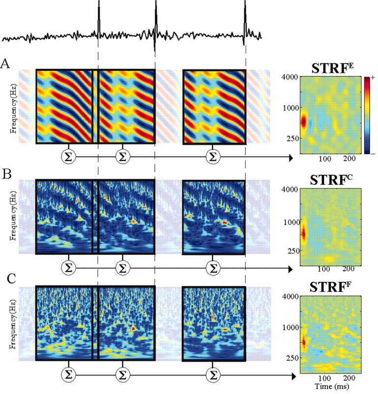
Schematic illustrating the use of reverse-correlation to derive STRFs. Top, Trace of a neuronal response. A–C, Three spectrotemporal representations of the TORC stimuli. In all three cases, the stimulus profiles preceding the occurrence of action potentials are averaged. Because the stimulus time evolves from left to right, the actual spike-triggered average is a stimulus spectrogram represented from –250 to 0 msec, where 0 msec corresponds to the actual occurrence time of the spike. The final STRF is a time-reversed average stimulus spectrogram, in which the time axis is flipped and the STRF can then be interpreted as the receptive field of the neuron. A, The envelope-based STRF^E averages the spectrotemporal envelope profile of the TORCs. B, STRF^C is based on averaging the complete auditory spectrogram of the stimulus. C, STRF^F is based on averaging the fine structure of the TORC auditory spectrograms. Note that the spectrograms shown in the figure correspond to the output of the filter-bank analysis. For display purposes, the outputs of the filters are passed through a half-wave rectification to exhibit the fluctuations in the stimulus spectrograms better.

Figure 6.

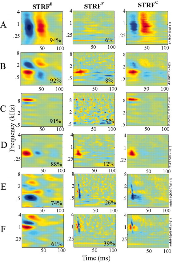
Examples of STRFs, with gradually increasing contributions of fine structure (from 5 to 40%). Each STRF triplet in each row corresponds to the STRF^E, STRF^F, and STRF^C derived for one neuron. An estimate of the contributions of STRF^Eand STRF^F to the total power of the STRF^C is indicated in each panel (see Materials and Methods). Each triplet is individually scaled to span the full range of colors in the color map. The fine-structure characteristics of the cells shown in this figure are as follows: A, λ = 3.9 spikes/sec, σ = 10 msec, α = 0.16, and ΔP_E = 94%; B, λ = 10.7 spikes/sec, σ = 10 msec, α = 0.07, and ΔP_E = 92%; C, λ = 27.5 spikes/sec, σ = 1 msec, α = 0.01, and ΔP_E = 91%; D, λ = 8.84 spikes/sec, σ = 4 msec, α = 0.3, and ΔP_E = 88%; E, λ = 10.3 spikes/sec, σ = 1 msec, α = 0.05, and ΔP_E = 74%; F, λ = 12.8 spikes/sec, σ = 1 msec, α = 0.03, and ΔP_E = 61%.

From a systems theory point of view, the STRF can be viewed as a second-order Volterra kernel of the neuron (Klein et al., 2000; Theunissen et al., 2000). Therefore, using reverse correlation for STRF estimation requires that one carefully consider the spectral and temporal structure of the stimulus ensemble. Traditionally, Gaussian white noise (GWN) has been used as a customary choice of stimulation because of its regular statistical properties (deBoer and De Jongh, 1978; Klein et al., 2000; Theunissen et al., 2000). However, such stationary noise sounds are not optimal stimuli to evoke strong responses in central nuclei such as the primary auditory cortex. Instead, it is the dynamic envelope of the acoustic spectrum that evokes robust cortical responses, and hence the TORC stimuli effectively present a noise-like envelope that can be formally treated much as the GWN was at previous auditory centers (deBoer, 1967; Klein et al., 2000). The autocorrelation function of TORC envelopes approaches an impulse function both spectrally and temporally, and thus formally approximates a white-noise stimulus (Klein et al., 2000). The autocorrelation of the TORC fine structure also possesses similar properties, in which the cross-channel correlation depends only on the channel difference, x – x′ (Fig. 1C). Therefore, no normalization of the spike-triggered stimulus average is required to complete the reverse-correlation process.

Relating the three STRFs

A more analytical description of the STRF can be viewed in the transfer function domain by taking a two-dimensional Fourier transform of the STRF:

(3)

The STRF is denoted in the Fourier domain by TF (transfer function), and represents the spectrotemporal modulation transfer function of the neuron. The coordinates ω and Ω correspond respectively to the temporal modulation rate (in cycles/sec) and spectral density content (in cycles/octave) of the STRF. Figure 4 A illustrates the STRF^E in the Fourier domain. Because the TORC envelopes contain ripples only over the range ω₀ = [–24,24] Hz, and Ω₀ = [–1.4,1.4] cycles/octave, we expect the span of the TF^E to be limited. [The choice of these ranges is based on previous experimental findings of the range of spectrotemporal modulations that elicit strong phase-locked responses in A1 units (Kowalski et al., 1996; Depireux et al., 2001)].

Figure 4.

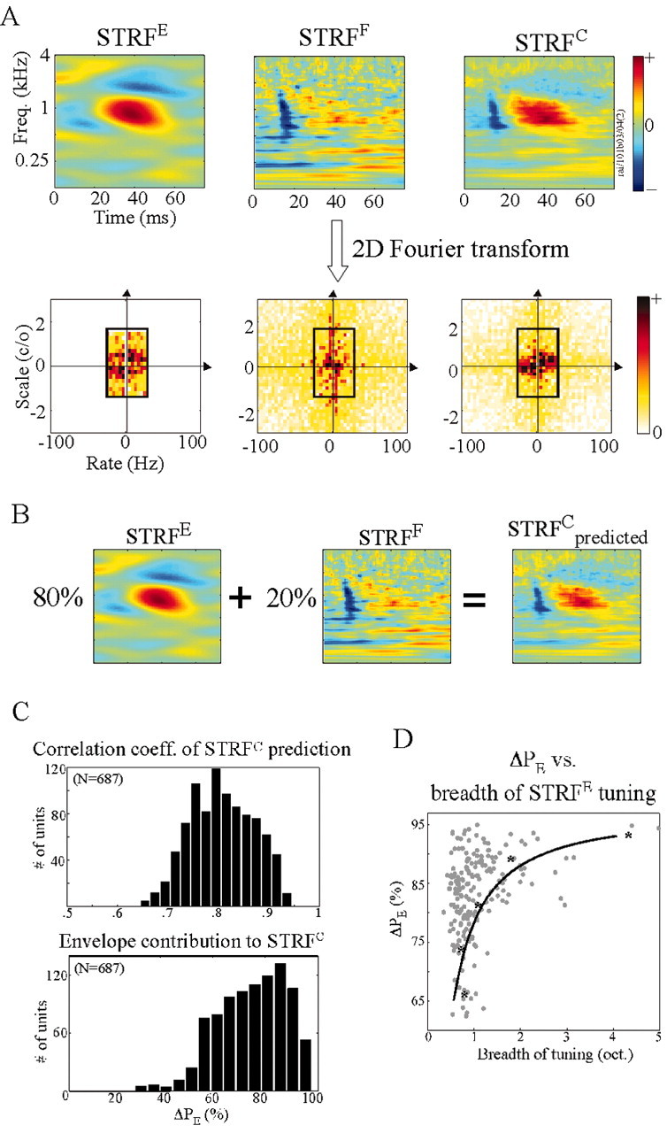
Example of an STRF triplet of a neuron and its significance. A, The three STRFs (STRF^E, STRF^F, and STRF^C) of a neuron, depicted both in the time-frequency and Fourier domains. The black box delimiting a subregion of the Fourier domain marks the range of spectrotemporal modulations spanned by the TORC stimuli. The fine-structure characteristics of the cell shown in this figure are as follows: λ = 17.8 spikes/sec; σ = 3.5 msec; α = 0.02; and ΔP_E = 80%. B, Estimating the contributions of the envelope and fine structure to reconstruct the STRF^C. C, Top, Distribution of the correlation coefficient relating the STRF^C to its prediction using ΔP_E (see Materials and Methods). Bottom, Distribution of values of ΔP_E observed in our data set. D, Scatter plot of ΔP_E variations as a function of breadth of tuning of the STRF^E. The solid curve is the best exponential fit to the means of the data within ±3.5% around each ΔP_E. The mean points are shown as asterisks.

By construction, the STRF^C spans a much wider range of spectrotemporal modulations than are included in the strictly envelope modulations of the STRF^E. Specifically, the STRF^C includes both the envelope as well as the much faster fine-structure modulations. We define the total power in the STRF^C as:

(4)

where TF^C is the two-dimensional Fourier transform of STRF^C. Then, the power in the STRF^C over the range spanned only by the TORC envelopes (ω₀, Ω₀) is denoted by p_E and is defined as:

(5)

The ratio ΔP_E = P_E/P_T is an estimate of the contribution of the STRF^E envelope patterns to the total response represented by STRF^C. The remainder of the power (1 – ΔP_E) is ascribed to the faster modulations of the STRF^F. Clearly, this estimate assumes the two ranges of STRF^E and STRF^F modulations are mutually exclusive, and hence ignores the relatively small contribution of the fine structure to the slow modulations in the STRF^E range. Nevertheless, this approximation is adequate for our purposes, and we will assume that the STRF^C is composed of a linearly weighted sum of STRF^E and STRF^F in the proportions of their power estimates (ΔP_E and 1 – ΔP_E) (see Fig. 4 B):

(6)

A robust linear behavior of the STRFs would result in STRF^C_predicted being similar to the measured STRF^C. We use a correlation coefficient (Papoulis, 1991) as a measure of similarity between the original STRF^C and STRF^C_predicted. The correlation coefficient takes values between +1 and –1, with +1 indicating a perfect match between the two STRF measures.

Dynamic synapse model

To investigate the role of synaptic adaptation in determining the characteristics of cortical temporal dynamics, we use a model that includes depressing and facilitating synaptic mechanisms described previously by Tsodyks et al. (1998). The model characterizes each synapse by a finite amount of resources (which can be thought of as an amount of synaptic neurotransmitters). A fraction of these resources is depleted after each presynaptic spike, and can be recovered with a time constant τ_d. Such a process describes the depression properties of the synapse and is governed by the dynamic equation:

(7)

where d(t) describes the fraction of resources available or recovered at time t. It can also be regarded as a use-dependent depression function controlled by the depression time constant τ_d. The other parameters are I(t) the input presynaptic firing rate at time t, and u(t) the synaptic utilization function. u(t) is a time-dependent release probability and depends on the depression function d(t) and a facilitation function f(t). Changes in the value of u(t) reflect, for example, the accumulation of calcium ions, which are responsible for the release of synaptic neurotransmitters (Bertram et al., 1996; Tsodyks and Markram, 1997; Tsodyks et al., 1998). Facilitation is modeled as a time function f(t) whose dynamics are captured by the equation:

(8)

where f(t) increases after each presynaptic spike and decays with a time constant τ_f. α_u is a constant defining the synaptic efficacy. In the case of purely depressing synapses, the value of u(t) = α_u, ∀t. To account for both facilitation and depression, the time-dependent utilization function u(t) is described by:

(9)

Equations 7, 8, and 9 capture the dynamics of a synaptic connection with both depression and facilitation properties. The parameters τ_d, τ_f, and α_u control the dynamics of the synapse, and can be chosen to model a purely facilitating or depressing synapse. In the absence of both facilitation and depression, the synapse operates in a simple linear manner.

The final synaptic input/output transformation is described by a time-dependent gain, in which the postsynaptic firing rate is proportional to the presynaptic firing rate, the utilization function u(t), the depression function d(t), and a constant W reflecting the absolute synaptic strength. It can be written as:

(10)

Finally, the output O(t) is passed through a low-pass filter with a 5 msec time constant (MacGregor, 1987) to generate the final neuronal membrane potential. In this model, we do not explicitly model action potentials, instead we assume the membrane potential represents the firing rate of the neuron when it exceeds a firing threshold, thus focusing only on the mechanisms of synaptic transmission and their role in explaining the temporal characteristics of cortical units.

In our simulations, we tested the synaptic utilization α_u with different values (range, 0.2–0.95) in accordance with the range of utilization estimates seen in vivo, and reported by Tsodyks and Markram (1997). Because varying the values α_u within this range had little effect on the results, we used α_u = 0.2. The facilitation mechanism is controlled by the time constant τ_f, which we set equal to 500 msec (Thomson and Deuchars, 1994; Tsodyks et al., 1998). For the depression time constant, we used a value τ_d = 65 msec for our initial simulations, but we also explored the full range of possible depression constants (40–200 msec) (Thomson and Deuchars, 1997; Abbott et al., 1997; Carandini et al., 2002) in relation to their effect in controlling the temporal tuning of cortical units.

Model of cortical circuitry

Cortical STRF^Es are likely the result of both excitatory and inhibitory interactions involving a variety of dynamic depressing as well as facilitating synapses. Specifically, thalamocortical (excitatory) synapses are believed to be mainly depressing (Thomson and Deuchars, 1994), whereas intracortical inhibitory connections appear to be strongly facilitating (Tsodyks et al., 1998; Reyes et al., 1998), especially between pyramidal neurons and inhibitory interneurons (Thomson and Deuchars, 1994).

We simulate a simplified model of an excitatory/inhibitory interaction at the input layer of A1, consisting of a depressive excitatory thalamocortical projection, added to a slower facilitative inhibitory corticocortical input. We presume that such excitatory and inhibitory interactions give rise to the wide variety of STRF^Es that emerge in the auditory cortex (Kowalski et al., 1996; Theunissen et al., 2000; Miller et al., 2001, 2002). For simplicity, we will model the basic excitatory and inhibitory influences as impulse responses with single-pole low-pass transfer functions H_e and H_i (see Fig. 10 B, right) with corner frequencies of 15 and 5 Hz, respectively. The two inputs are added together, followed by half-wave rectification (mimicking a spiking threshold) to remove negative firing rates. Synaptic dynamics are governed by the same depressive and facilitative mechanisms discussed in the previous section. The transfer function computations are based on this final rectified output.

Figure 10.

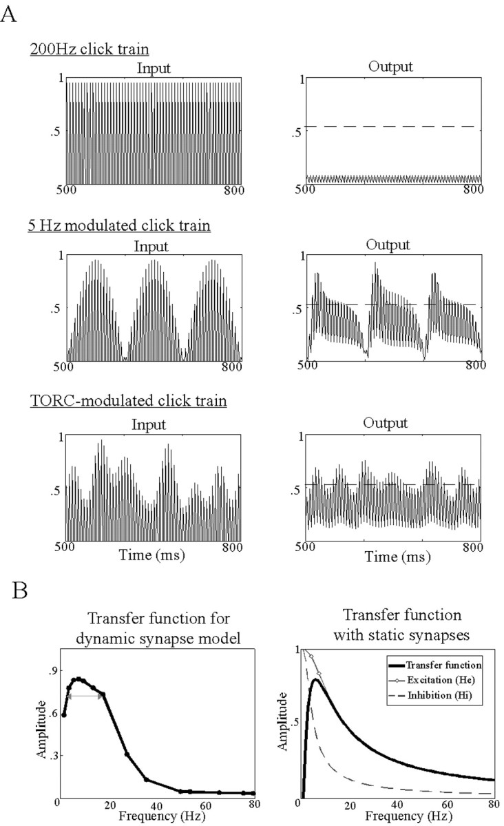
Simulation using dynamic synapse and cortical models. A, Dynamic synapse model input (presynaptic stimulus) and output (postsynaptic responses) to various modulations of a 200 Hz click train. Each row corresponds to the model responses to an unmodulated 200 Hz click train, 5-Hz-modulated click train, and TORC-modulated click train, respectively. B, Left, Transfer function of the single dynamic synapse model in response to click-train stimuli. The arrow highlights the bandwidth of the function, obtained with depression time constant τ_d = 65 msec (varying the time constant between 40 and 200 msec changes the bandwidth of the function, while maintaining its bandpass shape). Right, Transfer function of the excitatory/inhibitory cortical circuit with static weights, as well as the individual excitatory and inhibitory components (He and Hi).

Results

Data presented here were collected from a total of 918 single units in eight ferrets (37% from anesthetized animals). The awake recordings were typically characterized by a more vigorous firing rate; but apart from this difference, our analysis and findings apply to both anesthetized and awake conditions, unless otherwise stated.

Most units encountered in both anesthetized and awake recordings respond in a sustained manner to the TORC stimuli, as illustrated by the 1 sec response segments for the two units in Figure 2A. The responses exhibit simultaneously two patterns of phase locking. First, they are phase-locked to the TORC envelopes, as evidenced by the changing raster display from one TORC to the other. Second, the spikes are also precisely locked to the fine temporal patterns, common to all TORCs, giving the appearance of vertically aligned episodes in the raster plots across two or more TORCs. Moreover, this dual pattern of locking explains the disappearance of the vertically aligned episodes in some TORCs. This can be seen more easily in Figure 2A (right), where the H-TORC elicits responses locked to the fundamental frequency (48 Hz) of the harmonic sequence that makes up the TORC carrier (and hence its fine structure). The PSTH in Figure 2A (bottom right) accumulates responses over all repetitions of all TORCs, and illustrates the regularly spaced 48 Hz peaks caused by the periodicity of the fine structure. Note that although all raster spikes tend to occur at the regular 48 Hz intervals, they are completely missing in some TORCs, seemingly because the TORC envelope gates the occurrence of the spikes, as we will discuss later in more detail.

Quantifying phase-locking to fine structure

Cortical neurons vary widely in the extent and accuracy of phase locking to the stimulus fine structure. To quantify these properties, we computed and fitted the average cross-correlation function of each unit, using the procedures and model described in Materials and Methods. Figure 2B shows examples of cross-correlation functions of the two neurons whose raster responses are shown in Figure 2A. Both units exhibit a narrow peak at zero correlation lag (half-widths of ∼4 and 2 msec, respectively). Because the correlation is calculated across responses to different TORCs (and hence averages out all TORC envelopes), the width of the peak is a direct indication of the neuron locking to the fine-structure waveforms of the stimuli.

To quantify the jitter (σ) and spike reproducibility (α) across different trials and TORCs, as well as the average spike rate (λ) of each neuron, we fit the correlation by the Poisson-based model of spike cross-correlation shown in Figure 2C (see Materials and Methods). Figure 2D illustrates the range of values for these three parameters observed in all units. Over 63% of anesthetized and 77% of awake recordings exhibited precise locking of <10 msec accuracy (σ ≤ 10 msec). Note also that the awake population exhibited on average higher precision (Fig. 2D, middle, σ_mean of 18.7 vs 11.7 msec).

The distribution of the spike reproducibility parameter (α) was also biased toward 0 under all experimental conditions (Fig. 2D, right). This is partly caused by the fact that envelopes of different TORC stimuli are uncorrelated; and hence spikes are suppressed (gated out) differently from one TORC response to another. Therefore, computing a correlation function across responses to all stimuli would exhibit a reduction of spike reproducibility. As expected, the spike rate in the awake population was significantly higher than in the anesthetized (Fig. 2D, left, λ_mean of 18 vs 9) (Elhilali et al., 2002).

Spectrotemporal response fields of A1 units

We examined the response fields that emerge when taking into account neuronal responses to the envelope alone (STRF^E), fine structure alone (STRF^F), or the combined features (STRF^C). These STRFs (Fig. 3) reveal the differential spectrotemporal selectivity that cortical cells exhibit to these two sources of information in the acoustic stimulus, as we will discuss below. Figure 4A illustrates an example of an STRF triplet derived from the responses of one neuron. The STRF^E and STRF^F are strikingly different, although they share common features such as their center frequency (∼1 kHz). The STRF^C combines elements from both the STRF^E and STRF^F.

To demonstrate the relationship between these three STRF descriptions, we computed the proportion of the power contributed to the STRF^C by the envelope and fine-structure sources. The two-dimensional Fourier transforms of all three STRFs of this neuron are shown in Figure 4A (bottom). The black box delimits the energy region spanned by the TORC envelopes. By construction, the envelope-based STRF^E is defined only over the range [–24,24] Hz and [–1.4,1.4] cycles/octave, and thus contains no energy outside this area. In contrast, the fine-structure spectrograms include both coarse and fine temporal and spectral patterns, and thus the energy content of the STRF^F spreads over a wider range of spectral and temporal modulations. ΔP_E is computed from this representation as the ratio of the power within the box to the total power.

For this neuron, ΔP_E = 0.8, which results in a predicted STRF^C (Fig. 4B) that strongly resembles the measured STRF^C (Fig. 4A). Such resemblance has been observed for most units that exhibited highly precise responses, and for which we successfully derived an STRF^F (∼70% of units). This result supports the notion that the linear component of responses in A1 is very robust and strongly captured by the STRF descriptors. Figure 4C (top) shows the distribution of correlation coefficients between the STRF^C and the linearly predicted complete STRF derived from all units. The distribution indicates a high degree of correlation, with mean coefficient of +0.83 confirming the high degree of linearity in A1 responses, and thus suggesting an independence of the expression of envelope and fine structure in cortical responses.

The range of values of ΔP_E found in all units is shown in Figure 4C (bottom). This distribution is biased toward higher values of ΔP_E, indicating that the majority of units are driven primarily by their responses to time-varying spectral envelopes. This result is consistent with the accepted notion that A1 is particularly sensitive to slowly varying modulation patterns (Kowalski et al., 1996; Depireux et al., 2001; Eggermont, 2002). Nevertheless, over half of all cells exhibit a significant contribution (>25%) to their STRF^C from the fine-structure modulations, indicating that regular envelope-based STRF measurements are insufficient to capture all relevant spectrotemporal features of their response fields.

Robustness of the fine-structure receptive fields

The method used to derive the STRF^F (and STRF^C) requires the use of a spectrotemporal decomposition of the stimulus waveform to correlate the neural responses with the stimulus spectrotemporal features. To obtain a spectrographic representation of the stimulus, we used a filter-bank structure mimicking cochlear-like processing. The filters used were implemented as constant-Q filters with Q = 4. We tested the dependence of our STRF^F derivation on the choice of the filter-bank structure. Figure 5 shows the STRF^F of one unit obtained using filters with gradually varying bandwidths. The figure shows that a relatively stable representation of the STRF^F can be obtained as long as the filter bandwidths are within a biologically plausible range. As the bandwidth gets extremely narrow (Q = 12), or excessively broad (Q = 0.1), we start losing the features of the STRF^F, which translates to no correlation between the neural responses and the stimulus fine structure obtained through very narrow and very broad filters.

Figure 5.

STRF^F of a unit obtained using different filter-bank structures. The different panels correspond to decreasing values of filter Qs. The actual bandwidth used for the analysis in this study is Q = 4.

Not all units yield meaningful STRF^Fs. Units with very weak or absent fine-structure responses generate unreliable STRF^F, as measured using a bootstrap procedure on the STRF (Depireux et al., 2001). Weak STRF^Fs also occur in many broadly tuned cells that integrate over a wide range of frequency channels, and thus wash away any manifestation of the stimulus fine structure at any particular channel (see example in Fig. 6A and next section). The scatter plot of Figure 4D demonstrates that the expression of the fine structure (as quantified by the relative power contribution of the STRF^Fs to the complete STRF^C: 1 – ΔP_E) diminishes as the STRF^E bandwidth increases.

Examples of spectrotemporal properties of A1 units

STRFs in A1 exhibit a wide range of shapes and forms, reflecting the immense variety by which A1 units process and integrate various stimulus features along the spectrotemporal dimensions. Figure 6 displays several examples of receptive-field triplets (STRF^E, STRF^F, and STRF^C) obtained for different neurons. Generally, the STRF^C displays features that are prominent for both the STRF^E and STRF^F, depending on the contribution of each to the total power. The value in the lower right corner of each STRF^E and STRF^F indicates its contribution to the overall STRF^C of that neuron, as captured by the values of ΔP_E and 1 –ΔP_E.

Apart from the center frequency of the STRFs, we found no obvious relationship between the shapes of the STRF^E and STRF^F. Figure 6A–C shows a selection of neurons characterized by the large contribution of envelope features to their overall STRF^C, and hence the close similarity between their STRF^C and the STRF^E. Figure 6A is a classic example of a broadband offset unit, which preferentially responds to the offset of a stimulus over a wide frequency range. The broad tuning of this unit explains the weak contribution of the STRF^F because integrating from a large number of cochlear channels results in a complex waveform that is weakly correlated with any particular channel. Figure 6B illustrates an example of a spectrotemporally rich STRF with a similar STRF^C. The STRF^F here is rather simple, completely lacking the inhibitory fields of the STRF^E. Finally, Figure 6C depicts an example of a high-frequency cell, with a simple excitatory field at ∼8 kHz. The STRF^E shares very similar features with the STRF^F, with the exception of the much faster temporal dynamics in the latter. The periodic structure of the STRF^F is a result of the fact that the TORC carrier tones near 8 kHz are approximately equally separated within the narrow bandwidth of the STRF^E, hence creating a pseudo-periodic carrier waveform whose autocorrelation is also periodic.

The units depicted in Figure 6D–F are highly influenced by the fine-structure features, because they all exhibit a relatively high contribution of the STRF^F to the overall response (i.e., lower ΔP_E values). Figure 6D illustrates an example of change in temporal dynamics in response to the stimulus fine structure. The STRF^F of this unit shares the excitatory field with the envelopebased STRF^E at ∼500 Hz, but its temporal extent is much more narrow, and lacks any inhibitory surround. The example in Figure 6E illustrates a unit with very rapid temporal selectivity for the STRF^F. Finally, Figure 6F is a striking example of the independence of the fast and slow temporal features in cortical STRFs. The STRF^E of this unit exhibits two excitatory fields surrounding an inhibitory region near the best frequency (BF) at 1 kHz. However, its corresponding STRF^F indicates a specific selectivity to particularly fast oscillatory temporal patterns (at ∼150–200 Hz). This selectivity is reflected in the consecutive excitatory and inhibitory fields in the STRF^F (∼2 kHz). In turn, this pattern strongly dominates the STRF^C. Note, however, that despite the similarity of the STRF^F shapes of the different neurons in Figure 6E–F, their corresponding STRF^Es are very different, demonstrating again the independence of these two sources of information processing.

A closer analysis of the dynamics of the STRF^Fs gives an indication of the temporal resolution implied by the fine-structure responses. Specifically, we computed in each cell the Fourier transform of the STRF^F at the best frequency, and derived from that the 3 dB bandwidth and upper-cutoff points. The analysis was performed in a subset of all cells that have a high signal-to-noise ratio >2 (Depireux et al., 2001), and a good representation of the fine structure (σ < 20 msec). The scatter plots in Figure 7 reveal that both the measures increase as a function of the best frequencies of the units, largely because the cochlear bandwidths also increase in the same way. The figure also demonstrates that the upper cutoffs in some cells exceed 200 Hz, and that there is also a wide variability in the bandwidth and cutoff rates of the fine-structure responses at any given best frequency (up to a maximum that depends on the best frequency of the cell).

Figure 7.

The bandwidth (left) and upper-cutoff (right) rates of fine-structure responses derived from the STRF^F at BF. The solid curve is the best exponential fit to the means of the data within ±0.25 octaves around each best frequency. The mean points are shown as asterisks.

Responses to harmonic complexes

In 117 units, we recorded cortical responses using harmonic TORCs as well as regular TORCs (see Materials and Methods). Because of their regular structure, harmonic TORCs evoke periodic phase-locked responses that reflect the fundamental frequency of the stimulus carrier. Therefore, it is particularly easy to discern visually and computationally the degree of neuronal locking to fine temporal structure of the stimulus. For instance, one simple indicator of locking to the fine structure is the prominence of the Fourier coefficient at the fundamental frequency, computed from the Fourier transform of the average PSTH of all H-TORC responses. Recall that taking the average PSTH eliminates locking to the TORC envelopes, because these are uncorrelated across different TORCs. Figure 8A shows examples of this spectral analysis from 3 units. The red arrow points to the peak corresponding to the spectral component (Fourier coefficient) at the fundamental frequency used in the stimulus. All 3 units have strong locking to the harmonic fundamental frequency, up to 200 Hz. We have not yet tested units with higher fundamental frequencies, so the limit of this locking has yet to be determined. Of the 117 neurons tested, approximately half displayed noticeable locking to their harmonic fundamental frequency (over the range 25–200 Hz). This finding is remarkable for A1 units that are generally incapable of following sustained temporal modulations beyond 20 Hz.

Figure 8.

Harmonic TORC responses. A, Fourier transform of PSTHs of three neurons. Each neuron was tested with a different harmonic series, as indicated by the fundamental frequencies marked by the red arrows. All three neurons exhibit noticeably salient peaks at the fundamental component, and some of the upper harmonics. B, C, STRF^Es estimated using regular TORCs (left) and H-TORCs (right) for different neurons. The STRF^E pairs are very similar, with correlation coefficients of +0.92 and +0.91. The fine-structure characteristics of the cells shown in B and C are as follows: B, λ = 45.6 spikes/sec, σ = 3 msec, α = 0.2, and ΔP_E = 93%; C, λ = 20.3 spikes/sec, σ = 8.5 msec, α = 0.01, and ΔP_E = 90%.

We exploited the fact that the H-TORCs and regular TORCs stimuli share the same envelope structure to extract and compare their envelope-based STRF^Es. The goal of such a comparison is to determine whether cortical processing of the envelope is affected by the exact nature of the fine structure of the stimulus. Figure 8B,C demonstrates that the STRF^Es derived from either type of TORC are very similar for both units. Such similarity has been observed for all units for which we recorded a full set of TORCs and H-TORCs to derive a pair of STRF^Es using both types of stimuli. In all these cases, comparing the STRF^E obtained from TORCs and H-TORCs indicates a high degree of correlation between the two, with all correlation coefficients greater than +0.5, and mean +0.75. This finding strongly supports the notion that the cortical representation and processing of the envelope and the carrier do not seem to influence each other substantially. We will next explore the hypothesis that the envelope responses play a modulatory role for the expression of the fast fine-structure responses. Finally, note that it is not possible to obtain an STRF^F from H-TORC responses because all fine-structure patterns are at the same fundamental frequency.

Prediction of A1 responses

To illustrate directly the contribution of each of the STRF^E, STRF^C, and STRF^F to the description of the unit responses, we compared the actual responses to the TORC stimuli to those predicted using the STRFs (Fig. 9A). This is a common approach used previously to validate the linearity assumption underlying the definition and computation of the STRF (Kowalski et al., 1996; Theunissen et al., 2000; Depireux et al., 2001). We expected that the STRF^E would predict a smoothed version of the PSTH of TORC responses, whereas the STRF^C would predict a more detailed waveform that includes the fine structure. Figure 9B illustrates plots of the response of a cortical unit to H-TORCs along with the prediction of this response using the STRF^E and STRF^C. The arrows mark the anticipated locations of the fine-structure peaks because the carrier tones are multiples of a 48 Hz fundamental. As expected, the predictions demonstrate that the envelope waveform effectively gates or modulates the expression of the fine-structure peaks. Thus, when the predicted response to the envelope is small, the fine structure diminishes; when the response to the envelope is large, the peaks are well expressed in the PSTH.

Figure 9.

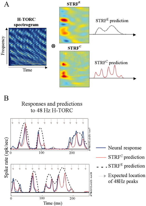
Comparison of actual and predicted responses to 48 Hz H-TORCs. A, Predicting responses to novel H-TORCs using STRFs measured with logarithmic TORCs. The spectrogram (envelope and complete, respectively) are convolved with the STRF (STRF^E and STRF^C, respectively) to predict the response of the cell to the H-TORC. B, Comparison of actual with predicted responses of two stimuli for the cell shown in A. Each plot illustrates a 250 msec period histogram of the responses. Responses (blue) and predictions (red) demonstrate the gating of the fine-structure peaks (arrows) by the responses to the envelope (dashed line).

Mechanisms underlying speed and precision of cortical dynamics

Why do dynamics of cortical responses differ from those observed in the thalamic inputs? Specifically, why do repetitive stimuli fail to elicit synchronized responses in A1 much beyond 20 Hz, a decade lower than typically found in the MGB? Such a significant slowdown is apparently not caused by simple global low-pass filtering of thalamic inputs because cortical cells are transiently still able to encode faithfully the rapid fine structure of the stimuli.

Two potential mechanisms are examined here, both known to be operative at the thalamocortical synapses and input layers. The first mechanism is the depressive character of the excitatory thalamocortical synapses. When subjected to continuous and/or rapid stimulation (or inputs), these synapses become temporarily depressed (weakened) as the supply of transmitter is exhausted. If the stimulus (thalamic input) is transiently turned off or reduced, the synapse can recover its strength in time for the next input. The potential rate at which the recipient cortical cell can respond to its fluctuating thalamic input depends critically on the dynamics of this recovery phase, as we will illustrate below in simulations of a simplified depressive synapse model (outlined in Materials and Methods).

The second potential mechanism involves coactivated excitatory and inhibitory influences that impinge on thalamorecipient cortical cells. Specifically, it is postulated that strong, feedforward, slightly delayed, and longer-lasting inhibition arrives after the onset of a persistent excitatory input. This inhibition reduces or suppresses the response, thus giving rise to the commonly seen phasic response at the onset of a stimulus. By slowly modulating the input strength (<20 Hz), one can alter the relative phase of the inhibition and excitation, and hence reduce the mutual cancellation and increase the response. However, much faster modulation rates induce sustained inhibition that attenuates the response again.

In the next two sections, we will elaborate on these two possibilities, using the simplified models outlined in Materials and Methods. Our goal here is not to replicate any specific data points, but rather to provide an intuitive understanding of the mechanisms that may give rise to these observed response properties.

Role of synaptic dynamics

We simulated the transformation of temporal dynamics caused by depressing excitatory thalamocortical and facilitative inhibitory intracortical synapses. The computational model of the dynamic synapse used (see Materials and Methods) (Tsodyks et al., 1998) is similar in details to several others that have been proposed and used to simulate auditory and visual cortical responses (Chance et al., 1998; Denham, 2001; Carandini et al., 2002; Chung et al., 2002). We will first reiterate the most relevant of the previous results involving the single depressive synapse model, and then extend the simulations to TORC-like stimuli that have both slow envelopes and fast fine structure.

The single synapse model confirms well known experimental and theoretical findings that cortical responses phase-lock well up to 15–20 Hz and are generally incapable of following much more rapid sustained periodic stimuli (Movshon et al., 1978; Schreiner and Urbas, 1988; Hawken et al., 1996; Kowalski et al., 1996; Lu et al., 2001; Eggermont, 2002). For instance, model responses diminish in amplitude gradually as the input pulse rate increases beyond 15 Hz. At lower rates (<2 Hz), the onset response to each input pulse becomes highly accentuated, and simultaneously, the response to the body of the pulse becomes relatively suppressed. The net result is that the model transfer function is maximal in an intermediate range of pulse rates. This is confirmed in Figure 10B (left) by the bandpass-shaped transfer function of the model, defined as the ratio of the amplitudes of the Fourier transform of the output (intracellular potential) to the input click train, as a function of click rate.

Of particular relevance to our TORC stimuli is the response of the model to slowly modulated, fast carrier signals such as those illustrated in Figure 10. In Figure 10A (first row), the stimulus is an unmodulated 200 Hz click train. As expected from the transfer function of the model (Fig. 10B, left), the model response is well below threshold, and does not induce spiking in the steady-state portion of the response. In contrast, Figure 10A (second row) illustrates the response to a 200 Hz periodic pulse with a relatively slow sinusoidal modulation (5 Hz) envelope. Note that the fast carrier waveform is still present in the response. In fact, it is particularly prominent at the onsets of the modulation pulses, and hence any spikes that might be initiated by these onsets would likely reflect the timing of these peaks. As the modulation waveform speeds up, onsets of subsequent pulses decrease in amplitude and the response weakens as predicted from the transfer function in Figure 10B (left).

The input in Figure 10A (third row) is another slowly modulated fast carrier, namely the response of one auditory channel to a TORC stimulus (as in Fig. 1). The envelope here is slowly varying (<24 Hz), riding on a 200 Hz fast pulse (corresponding to the fine structure). Unlike the unmodulated fine structure in Figure 10A (first row) or the sustained periodic envelope of the inputs in Figure 10A (second row), the envelope peaks at “random” intervals, and hence is not continuously depressed, but instead often fluctuates above the nominal threshold. It is also evident from the model results that the slow envelope gates the expression of the fine-structure peaks. Thus, when the (intracellular) response to the envelope is high, the fine structure associated with it rises and hence may exceed the spiking threshold causing precisely phase-locked action potentials to occur. Therefore, the ability of the model to respond to the fine structure is contingent on its ability to respond to the slow envelope.

Role of cortical circuitry

We have demonstrated thus far that depressing thalamocortical synapses can account for the nonlinear, relatively slow, yet precise dynamics of cortical responses. However, such synapses are only one part of neural circuits with excitatory and inhibitory interactions that give rise to the elaborate STRF shapes in the cortex. In fact, it has been postulated that such interactions, coupled with slow NMDA synapses, are themselves responsible for endowing the cortex with its characteristic dynamics and temporal tuning (Hirsch et al., 1998; Krukowski and Miller; 2001, Miller, 2003). The question therefore arises as to whether a simple model circuit of an excitatory thalamocortical input and a concurrent slower, intracortical, feedforward inhibitory input could give rise to the type of dynamics observed in the cortex. Figure 10B (right) illustrates that a network, with simple static synaptic weights between the two neurons and a final spiking threshold, can reproduce the bandpass linear transfer function seen previously with the depressing synapse model. Finally, reintroducing the dynamic synapses into the cortical circuit produces a bandpass transfer function very similar to those already seen in Figure 10B.

Discussion

The primary auditory cortex can respond precisely not only to sound onsets, but also to rapid sustained stimuli with precision of the order of a few milliseconds. This precise spiking to the fine structure of long-duration stimuli is contingent on the presence of relatively slow modulations of the stimulus spectrotemporal envelopes that can effectively excite the cortex. We used such a specially designed acoustic stimulus (the TORC) to elicit precise spiking throughout the stimulus presentation and simultaneously to explore the STRFs that give rise to these responses. In particular, by independently manipulating the fast carrier (or fine structure) of the TORC and its slow envelopes, we measured three different kinds of response fields: an STRF^E that reflects cortical processing of the slow envelopes, an STRF^F associated with processing of the fine structure, and an STRF^C that combines both sources of inputs.

Relationship to previous findings of rapid and precise firing in A1

Previous studies documenting this phenomenon in the auditory cortex have used a wide range of stimuli (narrowband or broadband; transient or repeated; AM, FM, or pure tones, clicks, or noise), measurement techniques (awake or anesthetized; intracellular or extracellular; single-unit, multiunit, or field evoked neural activity), and response measures (first-spike precision, temporal transfer functions, limits of phase-locking). Nevertheless, although a comparison of the results may often be highly speculative, there is, on the whole, a significant agreement among most on several fundamental response properties that are also consistent with our findings.

First, A1 units can generate precisely timed spikes (to within a few milliseconds) to transient events in the stimulus such as onsets and slowly repeating clicks (Heil, 1997; Phillips et al., 2002). Our results are consistent with these findings in that a sizable proportion of cells have narrow correlation peaks (small σ), indicating precisely timed spikes (Fig. 2D). This finding holds for spikes occurring throughout the presentation of the TORC stimulus and not simply near the onsets.

Second, temporal modulation transfer functions of cortical neurons exhibit a bandpass form, broadly tuned to various rates. The upper cutoff rate of the phase-following response is typically limited to a few tens of hertz (<30 Hz). These findings hold for a wide variety of response measures and regardless of whether the stimuli are modulated tones and noise or trains of tones, clicks, and noise (Schreiner and Urbas, 1988; Phillips, 1989; Eggermont, 2002). Cortical responses to ripples and TORCs are also consistent with these limits (Kowalski et al., 1996; Miller et al., 2002). When examined, the weakening of the phase-following response is not caused by a significant loss of spiking precision (or jitter), but rather to the dropping out of spikes when stimulus presentation rates are too fast (Phillips, 1989).

Third, cortical responses to “stationary” stimuli are mostly “phasic” in that they adapt out within 100 msec after stimulus onset, especially in anesthetized preparations, with a higher proportion of sustained responses in the awake animal (Bieser and Müller-Preuss, 1996; Lu et al., 2001). During this phasic epoch, it is possible to entrain responses to higher rates (>30 Hz) than is typically found with AM tones, ripples, and other temporally modulated stimuli, as discussed previously. For example, onset responses may phase-lock to pure tones at least up to 100–200 Hz (Wallace et al., 2002) and to higher rates with click trains (de Ribaupierre et al., 1972b; Lu et al., 2001). Recordings of activity of neuronal ensembles in A1 can also phase-lock up to ∼150 Hz (Fishman et al., 2000) in a sustained manner throughout the stimuli. Our data demonstrating precise and rapid phase locking to the TORC fine structure, (e.g., up to 200 Hz with harmonic TORCs in Fig. 8) are consistent with all of the above findings.

Finally, there have been several reports of in vivo intracellular recordings in A1 that suggest that intracortical inhibition plays a key role in shaping responses in the thalamorecipient layers (de Ribaupierre et al., 1972a,b; Wehr and Zador, 2002; DeWeese et al., 2003; Zhang et al., 2003). However, it has also been shown that in a significant fraction of A1 cells, locking rates are low in the absence of any inhibitory inputs [e.g., as in the thin-spike inhibitory interneurons (de Ribaupierre et al., 1972a)].

Synaptic mechanisms and cortical STRFs

Although precise, rapid, and sustained spiking is common in auditory cortical cells, it is encountered relatively infrequently because it requires stimuli that combine both a fine structure as well as a slowly modulated spectrotemporal envelope. In the absence of a fine structure, spikes phase-lock to the relatively slow envelopes of the inputs (2–20 Hz), and hence do not appear precisely timed except at sparsely spaced instants at which the envelope changes rapidly such as at stimulus onset. Similarly, stimuli with rapid fine structure but without spectrotemporal modulations (such as a sustained pure or complex tone, noise, or a fast click train) usually fail to elicit substantial response during their sustained portions, presumably because of adaptation, synaptic depression, or inhibitory influences (Ferster, 1994; Stratford et al., 1996; Gil et al., 1997). Therefore, in a sense, the slowly modulated envelopes of acoustic stimuli gate temporally precise and sustained cortical responses. When the stimulus envelope is such that the “gate” is open, cortical cells can precisely phase-lock to the stimulus fine structure up to relatively high rates (>200 Hz). When the gate is closed in the absence of slow modulations, responses soon cease.

Although synaptic depression and feedforward inhibition have been implicated and modeled to varying degrees at several sites along precortical auditory pathways (Nelson and Carney, 2003; McLeod and Carr, 2004), they are ubiquitous in all sensory cortices. This may explain the significant (order of magnitude) mismatch between the dynamics of the thalamus (medial and lateral geniculate nucleus) and cortex. It is therefore quite likely that the specialized processing of the spectrotemporal envelopes, as parameterized by the (envelope-based) STRF^E, is an emergent property exclusive to the cortex. In this light, the STRF^E and STRF^F can be viewed as representing two distinct sources of information processing. The STRF^E reflects the explicit cortical extraction and processing of the stimulus spectrotemporal envelope and the information it conveys. In contrast, the precise spiking (phase-locked to the input fine structure) represents temporal dynamics inherited from precortical stages (de Ribaupierre and Rouiller, 1981; Langner, 1992); thus, the STRF^F measured from these precise firings provides a window to the spectrotemporal nature of the thalamic inputs to the cortex. The different origins of the STRF^E and STRF^F explain the apparent independence between their shapes, as shown in Figure 6.

Functional significance of precise spiking in A1 and cortex in general

What is the functional significance and auditory perceptual correlates of precise cortical responses? Previously, we ascribed to synaptic depression and cortical circuitry the key innovation of the cortex: the creation of STRF^Es to analyze and represent the spectrotemporally modulated envelopes of acoustic signals. These slow modulations are the main carrier of information in speech and music. In speech, they reflect movements and shape of the vocal tract, and consequently the sequence of syllabic segments in the speech stream. In music, slow modulations reflect the dynamics of bowing and fingering, the timbre of the instruments, and the rhythm and succession of notes. Analogously, spatiotemporal modulations in visual images are correlates of changing scenes and moving objects.

Cortical cells respond well to change, manifested as modulated envelopes of carrier signals. The fine structure plays the important role of carrying these envelopes up to the cortex, in which they are extracted and analyzed. Therefore, it is possible that the precise spiking in the cortex reflects a precortical carrier (fine structure), and that it has certain perceptual correlates that the detection of rapid transient events in an otherwise slowly modulated signals such as speech (Viemeister and Wakefield, 1991), or the perception of “repetition” or “residue” pitch of <400 Hz (deBoer 1976; Shamma and Klein, 2000), and the “roughness” or “texture” of the acoustic signal [e.g., the continuum between whispered and a pure voiced quality corresponding to the range from random to periodic fine structure (Bieser and Müller-Preuss, 1996; Steinschneider et al., 1998; McKinney et al., 2001)].

One may also conjecture that the persistence of the fine structure in cortical responses is an epiphenomenon of the unique way the cortex extracts and processes the modulated envelopes. The cortex does not extract the envelope by rectifying and then low-pass-filtering its input signal. If it had done so, cortical responses would have been appropriately slow (2–20 Hz), but they would have also been very sluggish with respect to stimulus onsets, with rise times of the order of tens and hundreds of milliseconds (commensurate with the above modulation rates). Instead, synaptic depression provides a nonlinear mechanism that enables the cortex to slow down so as to track the most important envelope modulations, while simultaneously preserving its rapid onsets. This nonlinear mechanism effectively acts as a variable (or automatic) gain of the input envelopes, modifying its waveform according to the STRF, while leaving its fine structure (or carrier) mostly intact. In this sense, we hypothesize that the precise spiking seen in A1 and other sensory cortices is preserved in the responses as a side effect of using synaptic depression to process the envelopes.

References

- Abbott LF, Sen K, Varela JA, Nelson SB (1997) Synaptic depression and cortical gain control. Science 275: 220–224. [DOI] [PubMed] [Google Scholar]
- Abeles M (1982) Local cortical circuits: an electrophysiological study. Berlin: Springer.
- Bair W, Koch C (1996) Temporal precision of spike trains in extrastriate cortex of the behaving macaque monkey. Neural Comput 8: 1185–1202. [DOI] [PubMed] [Google Scholar]
- Bertram R, Sherman A, Stanley EF (1996) Single-domain/bound calcium hypothesis of transmitter release and facilitation. J Neurophysiol 75: 1919–1931. [DOI] [PubMed] [Google Scholar]
- Bieser A, Müller-Preuss P (1996) Auditory responsive cortex in the squirrel monkey: neural responses to amplitude-modulated sounds. Exp Brain Res 108: 273–284. [DOI] [PubMed] [Google Scholar]
- Carandini M, Heeger DJ, Senn W (2002) A synaptic explanation of suppression in visual cortex. J Neurosci 22: 10053–10065. [DOI] [PMC free article] [PubMed] [Google Scholar]
- Chance FS, Nelson SB, Abbott LF (1998) Synaptic depression and the temporal response characteristics of V1 cells. J Neurosci 18: 4785–4799. [DOI] [PMC free article] [PubMed] [Google Scholar]
- Chung S, Li X, Nelson SB (2002) Short-term depression at thalamocortical synapses contributes to rapid adaptation of cortical sensory responses in vivo. Neuron 34: 437–446. [DOI] [PubMed] [Google Scholar]
- deBoer E (1967) Correlation studies applied to the frequency resolution of the cochlea. J Aud Res 7: 209–217. [Google Scholar]
- deBoer E (1976) On the residue in hearing and auditory pitch perception. In Handbook of sensory physiology (Keidel W, Neff D, eds), pp 479–583. Berlin: Springer.
- deBoer E (1985) Auditory time constants: a paradox? In: Time resolution in auditory systems (Michelsen A, ed), pp 141–158. Berlin: Springer.
- deBoer E, De Jongh H (1978) On cochlear encoding: potentialities and limitations of the reverse-correlation technique. J Acoust Soc Am 63: 115–135. [DOI] [PubMed] [Google Scholar]
- deCharms R, Blake D, Merzenich M (1998) Optimizing sound features for cortical neurons. Science 280: 1439–1443. [DOI] [PubMed] [Google Scholar]
- Denham SL (2001) Cortical synaptic depression and auditory perception. In: Computational models of auditory function (Greenberg S, Slaney M, eds), Vol 312, pp 281–296. Amsterdam: NATO Science Series: Life Sciences, IOS. [Google Scholar]
- Depireux DA, Simon JZ, Klein DJ, Shamma SA (2001) Spectrotemporal response field characterization with dynamic ripples in ferret primary auditory cortex. J Neurophysiol 85: 1220–1234. [DOI] [PubMed] [Google Scholar]
- de Ribaupierre F, Goldstein MH, Yeni-Komshian G (1972a) Intracellular study of the cat's primary auditory cortex. Brain Res 48: 185–204. [DOI] [PubMed] [Google Scholar]
- de Ribaupierre F, Goldstein MH, Yeni-Komshian G (1972b) Cortical coding of repetitive acoustic pulse. Brain Res 48: 205–225. [DOI] [PubMed] [Google Scholar]
- de Ribaupierre F, Rouiller E (1981) Temporal coding of repetitive clicks: presence of rate selective units in cat's medial geniculate body (MGB). J Physiol (Lond) 318: 23–24. [Google Scholar]
- De Valois RL, De Valois KK (1990) Spatial vision. New York: Oxford UP.
- DeWeese MR, Wehr M, Zador AM (2003) Binary spiking in auditory cortex. J Neurosci 23: 7940–7949. [DOI] [PMC free article] [PubMed] [Google Scholar]
- Eggermont JJ (2002) Temporal modulation transfer functions in cat primary auditory cortex: separating stimulus effects from neural mechanisms. J Neurophysiol 87: 305–321. [DOI] [PubMed] [Google Scholar]
- Elhilali M, Fritz JB, Bozak D, Depireux DA, Simon JZ, Klein DJ, Shamma SA (2002) Comparison of response characteristics in auditory cortex of the awake and anesthetized ferret. Abstracts of the Twenty-sixth ARO Mid-Winter Meeting abstracts, Vol 25. Mt. Royal, NJ: Association of Research Otolaryngologists. [Google Scholar]
- Ferster D (1994) Linearity of synaptic interactions in the assembly of receptive fields in cat visual cortex. Curr Opin Neurobiol 4: 563–568. [DOI] [PubMed] [Google Scholar]
- Fishman YI, Reser DH, Arezzo JC, Steinschneider M (2000) Complex tone processing in primary auditory cortex of the awake monkey. II. Pitch versus critical band representation. J Acoust Soc Am 108: 247–262. [DOI] [PubMed] [Google Scholar]
- Fritz JB, Shamma SA, Elhilali M, Klein DJ (2003) Rapid task-related plasticity of spectrotemporal receptive fields in primary auditory cortex. Nat Neurosci 6: 1216–1223. [DOI] [PubMed] [Google Scholar]
- Gil Z, Amitai Y, Castro MA, Connors BW (1997) Differential regulation of neocortical synapses by neuromodulators and activity. Neuron 19: 679–686. [DOI] [PubMed] [Google Scholar]
- Hawken MJ, Shapley RM, Grosof DH (1996) Temporal-frequency selectivity in monkey visual cortex. Vis Neurosci 13: 477–492. [DOI] [PubMed] [Google Scholar]
- Heil P (1997) Auditory cortical onset responses revisited. I. First-spike timing. J Neurophysiol 77: 2616–2641. [DOI] [PubMed] [Google Scholar]
- Hirsch JA, Alonso JM, Reid RC, Martinez LM (1998) Synaptic integration in striate cortical simple cells. J Neurosci 18: 9517–9528. [DOI] [PMC free article] [PubMed] [Google Scholar]
- Klein DJ, Depireux DA, Simon JZ, Shamma SA (2000) Robust spectrotemporal reverse correlation for the auditory system: optimizing stimulus design. J Comput Neurosci 9: 85–111. [DOI] [PubMed] [Google Scholar]
- Kowalski N, Depireux DA, Shamma SA (1996) Analysis of dynamic spectra in ferret primary auditory cortex. I. Characteristics of single-unit responses to moving ripple spectra. J Neurophysiol 76: 3503–3523. [DOI] [PubMed] [Google Scholar]
- Krukowski AE, Miller KD (2001) Thalamocortical NMDA conductances and intracortical inhibition can explain temporal tuning. Nat Neurosci 4: 424–430. [DOI] [PubMed] [Google Scholar]
- Langner G (1992) Periodicity coding in the auditory system. Hear Res 6: 115–142. [DOI] [PubMed] [Google Scholar]
- Lewicki MS (1994) Bayesian modeling and classification of neural signals. Neural Comput 6: 1005–1030. [Google Scholar]
- Lu T, Liang L, Wang X (2001) Temporal and rate representations of timevarying signals in the auditory cortex of awake primates. Nat Neurosci 4: 1131–1138. [DOI] [PubMed] [Google Scholar]
- MacGregor RJ (1987) Neural and brain modeling. London: Academic.
- McKinney MF, Tramo MJ, Delgutte B (2001) Neural correlates of musical dissonance in the inferior colliculus. In: Physiological and psychophysical bases of auditory function (Breebaart DJ, Houtsma AJM, Kohlrausch A, Prijs VF, Schoonhoven R, eds), pp 83–89. Maastricht, The Netherlands: Shaker Publishing.
- McLeod KM, Carr CE (2004) Synaptic dynamics and intensity coding in the cochlear nucleus. In: Auditory signal processing: physiology, psychoacoustics, and models (Pressnitzer D, de Cheveigné A, McAdams S, Collet L, eds), pp 416–422. New York: Springer.
- Miller KD (2003) Understanding layer 4 of the cortical circuit: a model based on cat V1. Cereb Cortex 13: 73–82. [DOI] [PubMed] [Google Scholar]
- Miller LM, Escabi MA, Read HL, Schreiner CE (2001) Functional convergence of response properties in the auditory thalamocortical system. Neuron 32: 151–160. [DOI] [PubMed] [Google Scholar]
- Miller LM, Escabi MA, Read HL, Schreiner CE (2002) Spectrotemporal receptive fields in lemniscal auditory thalamus and cortex. J Neurophysiol 87: 516–527. [DOI] [PubMed] [Google Scholar]
- Movshon JA, Thompson ID, Tolhurst DJ (1978) Spatial and temporal contrast sensitivity of neurones in areas 17 and 18 of the cat's visual cortex. J Physiol (Lond) 283: 101–120. [DOI] [PMC free article] [PubMed] [Google Scholar]
- Nelson PC, Carney L (2003) A physiological model for neural responses to amplitude-modulated stimuli and for psychophysical modulation tuning. Abstracts of the Twenty-sixth ARO Mid-Winter Meeting abstracts, Vol 26. Mt. Royal, NJ: Association of Research Otolaryngologists. [Google Scholar]
- Oppenheim AV, Schafer RW (1999) Discrete time signal processing, Ed 2. Upper Saddle River, NJ: Prentice Hall.
- Papoulis A (1991) Probability, random variables, and stochastic processes. New York: McGraw Hill.
- Phillips DP (1989) Timing of spike discharges in cat auditory cortex neurons: implications for encoding of stimulus periodicity. Hear Res 40: 137–146. [DOI] [PubMed] [Google Scholar]
- Phillips DP, Hall SE, Boehnke SE (2002) Central auditory onset responses, and temporal asymmetries in auditory perception. Hear Res 167: 192–205. [DOI] [PubMed] [Google Scholar]
- Pinto DJ, Hartings JA, Brumberg JC, Simons DJ (2003) Cortical damping: analysis of thalamocortical response transformations in rodent barrel cortex. Cereb Cortex 13: 33–44. [DOI] [PubMed] [Google Scholar]
- Reyes A, Lujan R, Rozov A, Burnashev N, Somogyi P, Sakmann B (1998) Target-cell-specific facilitation and depression in neocortical circuits. Nat Neurosci 1: 279–285. [DOI] [PubMed] [Google Scholar]
- Schreiner CE, Urbas JV (1988) Representation of amplitude modulation in the auditory cortex of the cat. II. Comparison between cortical fields. Hear Res 32: 49–64. [DOI] [PubMed] [Google Scholar]
- Shamma SA, Klein DJ (2000) The case of the missing pitch templates: how harmonic templates may form in the early auditory system. J Acoust Soc Am 107: 2631–2644. [DOI] [PubMed] [Google Scholar]
- Shamma SA, Fleshman JW, Wiser PR, Versnel H (1993) Organization of response areas in ferret primary auditory cortex. J Neurophysiol 69: 367–383. [DOI] [PubMed] [Google Scholar]
- Steinschneider M, Reser DH, Fishman YI, Schroeder CE, Arezzo JC (1998) Click train encoding in primary auditory cortex of the awake monkey: evidence for two mechanisms subserving pitch perception. J Acoust Soc Am 104: 2935–2955. [DOI] [PubMed] [Google Scholar]
- Stratford KJ, Tracy-Hornoch K, Martin KAC, Bannister NJ, Jack JJ (1996) Excitatory synaptic inputs to spiny stellate cells in cat visual cortex. Nature 382: 258–261. [DOI] [PubMed] [Google Scholar]
- Theunissen FE, Sen K, Doupe AJ (2000) Spectral–temporal receptive fields of nonlinear auditory neurons obtained using natural sounds. J Neurosci 20: 2315–2331. [DOI] [PMC free article] [PubMed] [Google Scholar]
- Thomson AM, Deuchars J (1994) Temporal and spatial properties of local circuits in neocortex. Trends Neurosci 17: 119–126. [DOI] [PubMed] [Google Scholar]
- Thomson AM, Deuchars J (1997) Synaptic interactions in neocortical local circuits: dual intracellular recordings in vitro. Cereb Cortex 7: 510–522. [DOI] [PubMed] [Google Scholar]
- Tsodyks MV, Markram H (1997) The neural code between neocortical pyramidal neurons depends on neurotransmitter release probability. Proc Natl Acad Sci USA 94: 719–723. [DOI] [PMC free article] [PubMed] [Google Scholar]
- Tsodyks M, Pawelzik K, Markram H (1998) Neural networks with dynamic synapses. Neural Comput 10: 821–835. [DOI] [PubMed] [Google Scholar]
- Viemeister NF, Wakefield GH (1991) Temporal integration and multiple looks. J Acoust Soc Am 90: 858–865. [DOI] [PubMed] [Google Scholar]
- Wallace MN, Shackleton TM, Palmer AR (2002) Phase-locked responses to pure tones in primary auditory cortex. Hear Res 172: 160–171. [DOI] [PubMed] [Google Scholar]
- Wang K, Shamma SA (1994) Self-normalization and noise-robustness in early auditory representations. IEEE Trans Speech Audio Proc 2: 421–435. [Google Scholar]
- Wehr M, Zador A (2003) Balanced inhibition underlies tuning and sharpens spike timing in auditory cortex. Nature 426: 442–446. [DOI] [PubMed] [Google Scholar]
- Yang X, Wang K, Shamma SA (1992) Auditory representations of acoustic signals. IEEE Trans Inform Theory 38: 824–839. [Google Scholar]
- Zhang LI, Tan AY, Schreiner CE, Merzenich MM (2003) Topography and synaptic shaping of direction selectivity in primary auditory cortex. Nature 424: 201–205. [DOI] [PubMed] [Google Scholar]